Modelisation of the diffusive transport of algal blooms in a coastal environment using a stochastic method

HAL Id: pastel-00668176

https://pastel.archives-ouvertes.fr/pastel-00668176

HAL is a multi-disciplinary open access archive for the deposit and dissemination of sci-entific research documents, whether they are pub-lished or not. The documents may come from teaching and research institutions in France or abroad, or from public or private research centers.

L’archive ouverte pluridisciplinaire HAL, est destinée au dépôt et à la diffusion de documents scientifiques de niveau recherche, publiés ou non, émanant des établissements d’enseignement et de recherche français ou étrangers, des laboratoires publics ou privés.

a coastal environment using a stochastic method

Antoine Joly

To cite this version:

Antoine Joly. Modelisation of the diffusive transport of algal blooms in a coastal environment using a stochastic method. Other [q-bio.OT]. Université Paris-Est, 2011. English. �NNT : 2011PEST1088�. �pastel-00668176�

Université Paris-Est

Sciences, Ingénierie et Environnement

Thèse

Présentée pour l’obtention du grade de DOCTEUR DE L’UNIVERSITE

PARIS-EST

par

Antoine Joly

Modélisation du transport des algues en

milieu côtier par une approche stochastique

Spécialité

Mécanique des Fluides

Soutenue le 14 décembre 2011 devant un jury composé de :

Rapporteur

Jean-Marie MOUCHEL

(Université Paris 6)

Rapporteur

François SCHMITT

(Université Lille 1)

Examinateur

Michel BENOIT

(EDF R& D / ENPC)

Directeur de thèse

Damien VIOLEAU

(EDF R& D)

Examinateur

Dominique ASTRUC

(IMFT)

Examinateur

Jean-Pierre MINIER

(EDF R& D)

Président du jury

Pierre SAGAUT

(Université Paris 6)

Thèse effectué au sein du Laboratoire d’Hydraulique Saint-Venant c/o EDF R& D

6, quai Watier BP 49

78401 Chatou cedex France

RÉSUMÉ iii

Résumé

Ce mémoire de thèse a pour but de présenter un modèle de prédiction du transport des algues en mer le long des côtes. La méthode choisie a été d’utiliser un code industriel eulérien pour prédire l’écoulement moyen sur une grande surface, et d’ensuite ajouter un modèle lagrangien pour prédire le mouvement des particules individuelles. Ce modèle lagrangien comporte trois étapes. Premièrement, les caractéristiques moyennes du fluide trouvées avec le modèle eulérien sont utilisées pour alimenter un modèle stochastique pour trouver les vitesses turbulentes du fluide à l’emplacement des partic-ules modélisant les algues. Ensuite ces vitesses turbulentes sont utilisées à travers les composantes de la force de traînée, de l’inertie, de la force de Basset et de la poussée d’Archimède pour trouver les vitesses des corps. La dernière étape consiste à utiliser ces vitesses des corps pour calculer leurs trajectoires. Une méthode avec un intégrateur exact a été développée pour résoudre ces équations. Ce modèle a ensuite été validé grâce à deux expériences. Dans la première expérience, des sphères de tailles différentes ont été lâchées dans deux fluides avec des densités différentes, où une turbu-lence stationnaire quasi-homogène a été générée en utilisant une paire de grilles oscillantes. Dans la deuxième expérience des particules sphériques ont été lâchées dans un écoulement non-homogène. Cette écoulement a été obtenu en obstruant partiellement un canal, afin qu’une zone de recircula-tion soit générée. Le modèle de transport des particules a ensuite été testé sur des simularecircula-tions d’un écoulement réel le long des côtes normandes, dans lequel des particules numériques représentant des algues ont été lâchées.

Mots clés :

Transport stochastique de particules, Couplage eulérien-lagrangien, Intégrateur exact, Turbulence de grilles, Canal partiellement obstrué, Transport côtier des algues

v

Modelling of the transport of algae in a coastal

environment using a stochastic method

ABSTRACT vii

Abstract

The aim of this PhD thesis was to develop a model to predict the motion of algae in sea waters along a coastline. The method chosen was to use a large Eulerian industrial code to model the mean flow, and add Lagrangian model to predict the motion of individual particles. This Lagrangian model is a three-step model. In the first modelling step, the mean flow characteristics at the location of the particles (solid bodies modelling the algae) are extracted from the Eulerian model and imputed into a stochastic model to find the turbulent fluid velocities. These fluid velocities are used in the second step to solve for the solid body velocities, by solving for the drag, momentum, buoyant and Basset history forces. The final modelling step is to use these solid body velocities to calculate the trajectories of particles. An exact integrator method was then developed to solve for these equations. The model was then validated using two experiments. Firstly sphere of different size were released in fluids of different densities, where a stationary quasi-homogeneous turbulence. This turbulence was generated by oscillating a pair of grids. In the second experiment spherical particles were released in a non-homogeneous turbulent flow. This flow was achieved by partially obstructing a channel, so that a recirculation zone was generated. The particle transport model was then tested numerically using the simulations of a real flow along the coasts of Normandy where numerical particles representing algae were released.

Keywords:

Stochastic particle transport, Eulerian-Lagrangian coupling, Exact integrator method, Grid generated turbulence, Partially obstructed channel flow, Coastal algae transport

REMERCIEMENTS ix

Remerciements

out d’abord je tiens à remercier Monsieur Damien Violeau, mon directeur de thèse, qui est parvenu à être très disponible pendant toute la durée de ma thèse et qui a su répondre à toute mes questions. Je tiens aussi à remercier Monsieur Michel Benoit, le directeur du Laboratoire d’Hydraulique Saint-Venant et mon co-encadrant de thèse, qui a su me faciliter la thèse pendant ces trois ans.

J’aimerai aussi remercier Messieurs Jean-Marie Mouchel et François Schmitt pour avoir accepté d’être rapporteurs de mon travail. Je voudrai aussi remercier Monsieur Pierre Sagaut qui qui a assuré la présidence du jury de thèse.

Je voudrai aussi remercier tout particulièrement Monsieur Jean-Pierre Minier pour toute l’aide qu’il m’a apporté pendant ma thèse ainsi que le temps qu’il a pris pour m’expliquer les modèles stochas-tiques. Je le remercie aussi d’avoir accepté de faire partie de mon jury de thèse.

Je tiens aussi à remercier Messieurs Dominique Astruc, Frédéric Moulin et Sébastien Cazin, ainsi que le reste de l’équipe de l’IMFT, pour toute l’aide qu’ils m’ont fournie dans la conception et la réalisation des expériences. Je remercie aussi Monsieur Dominique Astruc d’avoir accepté de faire partit de mon jury de thèse.

Je remercie Monsieur Rob Uittenbogaard pour toutes les questions avisées qu’il a pu poser pendant tout le suivi de ma thèse ainsi que pour son déplacement depuis les Pays-Bas pour pouvoir faire partie de mon jury de thèse.

Je continuerai mes remerciements en mentionnant tous les membres d’EDF et du Laboratoire d’Hydraulique Saint-Venant que j’ai pu côtoyer et qui ont su créer une très bonne ambiance de travail, tout en restant professionnels et dynamiques.

Merci ensuite à Jean-Romain, et au reste de l’équipe du Pomphy pour toute l’aide qu’ils m’ont ap-portée pendant mes expériences. Merci à Réza, qui a été un très bon chef de projet (même si ce fut court). Merci à Chi-Tuan qui m’a fait profiter de plein de places de rugby. Merci à Jean-Michel qui est arrivé à rester très disponible pour toutes les questions sur Telemac que j’ai pu avoir.

Merci aussi à Elodie d’avoir ouvert la voie et merci à Etienne d’avoir accompli sa thèse en parallèle de la mienne. Merci à mon voisin de bureau Cédric pour toutes les conversations rugby que l’on a eu ensemble. Merci aussi à Andrès d’être passé dans notre bureau chaque fois qu’il en avait marre de travailler. Merci à Christophe et Martin pour tous les joggings sur l’île des Impressionnistes

Merci aussi à toutes les autres personnes que j’ai pu côtoyer de près ou de loin à Chatou que ce soit le personnel permanent ou le personnel temporaire.

Merci à mes parents, mes grands-parents, Pascale, Fredo et Armel d’avoir assisté à ma soutenance, et surtout d’avoir essayé de comprendre ma présentation.

Merci enfin à ma chérie Amélie, grâce à elle j’ai pu m’aérer l’esprit et penser à autre chose que mon mémoire pendant la fin de ma thèse. Merci aussi pour tout le soutien et la tendresse qu’elle a pu m’apporter.

Contents

1 Introduction 2

2 Context 6

2.1 The algae problematic . . . 7

2.2 Modelling approach . . . 8

2.3 Categorising the problem . . . 8

2.4 Existing algae transport models . . . 9

2.5 Existing particle transport models . . . 10

3 Environmental Flow Modelling 12 3.1 General principles of fluid mechanics . . . 13

3.2 General principles of turbulence modelling - first-order models . . . 14

3.3 General principles of turbulence modelling - second-order models . . . 19

4 Dynamic Properties of Solid Particle Motion 24 4.1 Forces acting on the motion of a solid particle in fluid . . . 25

4.2 Simplification to an isotropic body . . . 30

4.3 Testing the impact of different force components . . . 30

4.4 Testing the physical characteristics of solid bodies . . . 33

5 Fluid Velocities Model 38 5.1 A brief overview of stochastic modelling in fluid mechanics . . . 39

5.2 The Simplified Langevin Model of turbulence . . . 40

5.3 Testing the Simplified Langevin Model . . . 45

6 Numerical Resolution 50 6.1 Two-phase modelling . . . 51

6.2 Preliminary numerical considerations . . . 52

6.3 The exact integrator method . . . 53

6.4 Asymptotic behaviour of the model . . . 56

CONTENTS xi

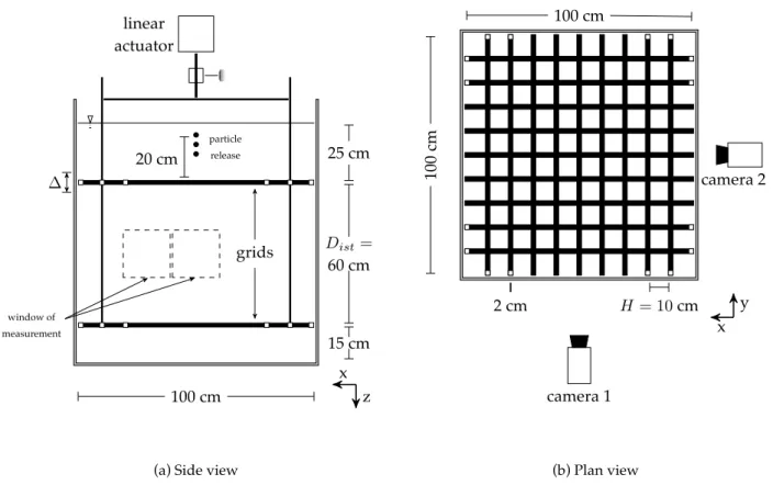
7.1 Experimental setup . . . 61

7.2 The turbulent regime . . . 61

7.3 Particle tracking . . . 65

7.4 Model Validation . . . 68

8 Particles Released in a Partially Obstructed Channel 78 8.1 Experimental setup . . . 79

8.2 The flow regime . . . 79

8.3 Particle tracking . . . 83

9 Real Life Applications 94 9.1 Information on the type of algae considered . . . 95

9.2 Applying the model to represent algae particles . . . 96

9.3 Application around a real bathymetry . . . 98

9.4 Description of the problematic around Paluel . . . 99

9.5 Transport patterns . . . 102

9.6 Particles exiting the domain . . . 112

10 Conclusion 120 10.1 Conclusion on the validity of the model . . . 121

10.2 Strong points of the model . . . 122

10.3 Limitations and perspectives . . . 123

10.4 Advices to use the model . . . 124

A Calculations relative to the exact integrator model 126 A.1 The three steps solid particle transport model . . . 127

A.2 Analytical solution for the fluid velocities . . . 127

A.3 Analytical solution for the solid particle velocities . . . 128

A.4 Analytical solution for the position of the body . . . 131

A.5 Solving the stochastic integrals . . . 133

B Asymptotic behaviour of the exact integrator model 142 B.1 For dt≫ T(s) i . . . 144 B.2 For dt≪ T(s) i . . . 146 B.3 For dt≫ τpart . . . 149 B.4 For dt≪ τpart . . . 152

C Video particle tracking image processing 158 C.1 Methodology for the image processing . . . 159

D Stopping particles at boundaries in a triangular mesh 174

D.1 Finding in which element a particle can be found . . . 175

D.2 Interpolate the nodal values inside an element . . . 176

D.3 Finding inside which element a particle is after its displacement . . . 178

D.4 Finding which boundary was crossed by a particle . . . 179

List of Figures

2 Context 6

2.1 Surface covered in Ulva in Brittany during the year 2009 . . . 7

3 Environmental Flow Modelling 12

3.1 An example of a recording of a turbulent fluid velocity in time . . . 15

4 Dynamic Properties of Solid Particle Motion 24

4.1 The evolution of VZand τpartfor spherical particles falling in a stationary fluid . . . . 33

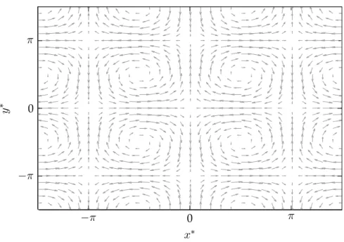
4.2 Typical shape of Taylor eddies . . . 34 4.3 The transport of solid particles with different physical characteristics in Taylor eddies 35

5 Fluid Velocities Model 38

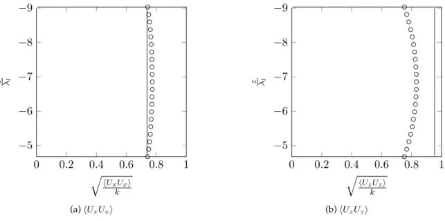
5.1 Second moments found for fluid particles released in stationary homogeneous isotropic turbulence . . . 46 5.2 Second moments of fluid particle velocities in stationary quasi-isotropic grid turbulence 47 5.3 The autocorrelation of the fluid velocities in stationary quasi-isotropic grid turbulence 48

7 Particles Falling in Quasi-Homogeneous Turbulence 60

7.1 Scheme of the double-grid setup . . . 61 7.2 An instantaneous PIV recording . . . 62 7.3 The kinetic energy and its dissipation rate in oscillating grid turbulence . . . 63 7.4 Vertical profiles for the characteristic values of turbulence in oscillating grid turbulence. 65 7.5 Dimensionless settling velocities for different particle fluid density ratios. . . 67 7.6 Volume of measurements for the two perpendicular cameras recording falling bodies. 67 7.7 Example of particles recorded for the two cameras. . . 68 7.8 Probability density functions for particle velocities present inside the volume of

mea-surement . . . 70 7.9 Probability density functions for numerical particle velocities present inside the

LIST OF FIGURES xv

7.10 Particle statistics used to illustrate the filtering of turbulent eddies by solid particles . 73 7.11 The correlation profiles of velocities for particles released in quasi-homogeneous

tur-bulence . . . 74

8 Particles Released in a Partially Obstructed Channel 78 8.1 Experimental setup . . . 79

8.2 The streamlines for the flow defined by the experimental set up shown in figure 8.1 . 80 8.3 Profiles of the horizontal velocity plotted at different locations along the canal . . . 81

8.4 Profiles of the turbulent kinetic energy plotted at different locations along the canal . . 82

8.5 Profiles of the turbulent kinetic energy dissipation rate plotted at different locations along the canal . . . 82

8.6 Experimental setup to record the particle trajectories . . . 83

8.7 Typical particle trajectories . . . 84

8.8 A disturbed image recorded by the camera due to the air entrainment . . . 84

8.9 An annotated example of the results of the partially obstructed channel experiment . 85 8.10 Partially obstructed channel: proportion of released particles entering a quadrant of the window of measurement . . . 87

8.11 Partially obstructed channel: mean particles residence time inside a quadrant of the window of measurement . . . 88

8.12 Partially obstructed channel: proportion of released particles entering a quadrant of the window of measurement . . . 89

8.13 Partially obstructed channel: mean particles residence time inside a quadrant of the window of measurement . . . 90

9 Real Life Applications 94 9.1 Example of algae . . . 95

9.2 The drag coefficient for an Iridaea flaccida . . . 96

9.3 Comparison between a free falling alga and an equivalent sphere . . . 97

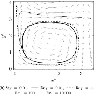
9.4 Trajectories of different bodies released in Taylor eddies . . . 98

9.5 The bathymetry around the Paluel power station . . . 99

9.6 Vector plots showing the importance of radiation stresses . . . 103

9.7 Particles transported in the flow around Paluel using model VII . . . 105

9.8 Particles transported in the flow around Paluel using model VIII . . . 106

9.9 Particles transported in the flow around Paluel using model IV . . . 107

9.10 Particles transported in the flow around Paluel using model III . . . 108

9.11 Particles transported in the flow around Paluel using model II . . . 109

9.12 Particles transported in the flow around Paluel using model V . . . 110

9.13 Particles transported in the flow around Paluel using model VI . . . 111

9.15 Bar plots of the number of particles entering each pumps, for different solid body

dy-namics models . . . 113

9.16 Bar plots of the number of particles entering each pumps, for different solid body shape or size . . . 114

9.17 Fluid velocity vectors around the pumps of the Paluel power station . . . 115

9.18 Mean location at which the particles exit the domain for different particle transport model . . . 116

9.19 Cumulative number of particles entering each pumps for models considering different particles . . . 116

C Video particle tracking image processing 158 C.1 The tools used to calibrate the cameras of the oscillating grids experiment . . . 159

C.2 Probability density functions of the errors on the positions of the fishing weights . . . 160

C.3 Steps necessary to obtain the position of the bodies from an image recorded by a camera162 C.4 Steps required to find the position of two superposed bodies . . . 163

C.5 Steps necessary to remove impurities the size of a particle . . . 164

C.6 A disturbed image due to the air entrainment . . . 165

C.7 The starting point to associate recorded particles . . . 166

C.8 Studying the different possible particle counterparts . . . 166

C.9 A position of a particle at time t, and the recognised bodies in each camera at time t = 1 167 C.10 Distance travelled from the intial position at time t . . . 168

C.11 Position of the particles present in the field of vision of both cameras . . . 169

C.12 Flow chart of the algorythm used to calibrate the volume of measurement . . . 170

C.13 Flow chart of the algorythm used to find the position of particles in an image recorded by a camera . . . 171

C.14 Flow chart of the algorithm used to find the three dimensional trajectories of bodies for the oscillating grids experiment . . . 172

D Stopping particles at boundaries in a triangular mesh 174 D.1 A particle inside a element of a first order triangular mesh . . . 175

D.2 A transformation of coordinates of an element using barycentric coordinates . . . 176

D.3 A triangular element, with three boundaries, surrounded by six neighbouring elements 178 D.4 A particle path crossing a triangular element boundary . . . 179

Nomenclature

Roman Symbols

bi Coefficient relating Ti(s)to Ti . . . (-)

bij Anisotropy tensor . . . (–)

B_i(s) Coefficient corresponding to the standard deviation of the stochastic part of the solid particle

velocity . . . (m·s−3/2₎

C0 Constant used in the Simplified Langevin Model, typically set to 2.1 . . . (-)

CB Basset history force constant . . . (kg·s1/2)

Ci,Bas The Basset history force components independent of the current time . . . (kg·m·s2)

CD,a Drag coefficient for an alga . . . (–)

ˇ

Ci A constant used in the exact integrator model . . . (-)

C_i(s) Coefficient regrouping all the mean flow components seen by a solid particle . . . (m·s−2) D Characteristic length of a solid body . . . (m) Da Diameter of a disk representing an alga . . . (m)

Dist Distance between the oscillating grids . . . (m)

Ds Diameter of a solid sphere . . . (m)

f Frequency of the grid oscillation . . . (s−1) Fa Coefficient of the solid particle velocity linked to the evolution of the fluid velocities . . . (-)

Fb Coefficient of the solid particle velocity linked to the velocity differences between the fluid and

the solid body . . . (s−1₎

Fi,c Coefficients of the solid particle velocity linked to constant values at time t . . . (m·s−2)

g Vectorial acceleration due to gravity . . . .(m·s−2₎

H Mesh size of the oscillating grids . . . (m) h Depth of the fluid . . . (m) k Turbulent kinetic energy . . . (m2_·s−2₎

ˇ

Ki A constant used in the exact integrator model . . . (-)

M Added mass constant for an isotropic body . . . (kg) m Mass of a solid body . . . .(kg)

NOMENCLATURE xix

Ma Added mass constant for an alga . . . (kg)

Mij Added mass tensor of a body . . . (kg)

Ms Added mass constant for a sphere . . . (kg)

N Number of subintervals in the numerical window of the Basset history force . . . (–) Nr Number of particles present in the flow . . . (pcs)

P Fluid pressure . . . (kg·m−1·s−2)

ˇ

Qi A constant used in the exact integrator model . . . (-)

Re Reynolds number of the flow . . . (–) Rea Particle Reynolds number of an alga . . . (–)

Rep Particle Reynolds number . . . .(–)

Res Particle Reynolds number of a sphere . . . (–)

Reset Particle Reynolds number once the terminal settling velocity has been reached . . . .(-)

S Cross-sectional area of a solid body . . . (m2₎

Sa Surface area of a disk representing an alga . . . (m2)

Sij Mean rate-of-strain tensor . . . (s−1)

sij Fluctuating rate of strain tensor . . . (s−1)

S Scalar mean rate of strain . . . (s−1₎

Ss Cross-sectional area of a sphere . . . (m2)

Stset Stokes number used to characterise the influence of the turbulence . . . (-)

T Integral of the autocorrelation of fluid velocities in stationary homogeneous isotropic

turbu-lence . . . .(s)

ta Thickness of a disk representing an alga . . . (m)

T_i(s) The integral time scale of the fluid velocities seen by a solid body . . . (s) Tt Turbulent characteristic time (linked to large eddies) . . . (s)

twin Time of the numerical window used to solve for the Basset history force . . . (s)

U Vectorial fluid velocity . . . (m·s−1₎

Ui Fluid velocity along the ithdirection . . . (m·s−1)

Ui Turbulence-averaged fluid density . . . (m·s−1)

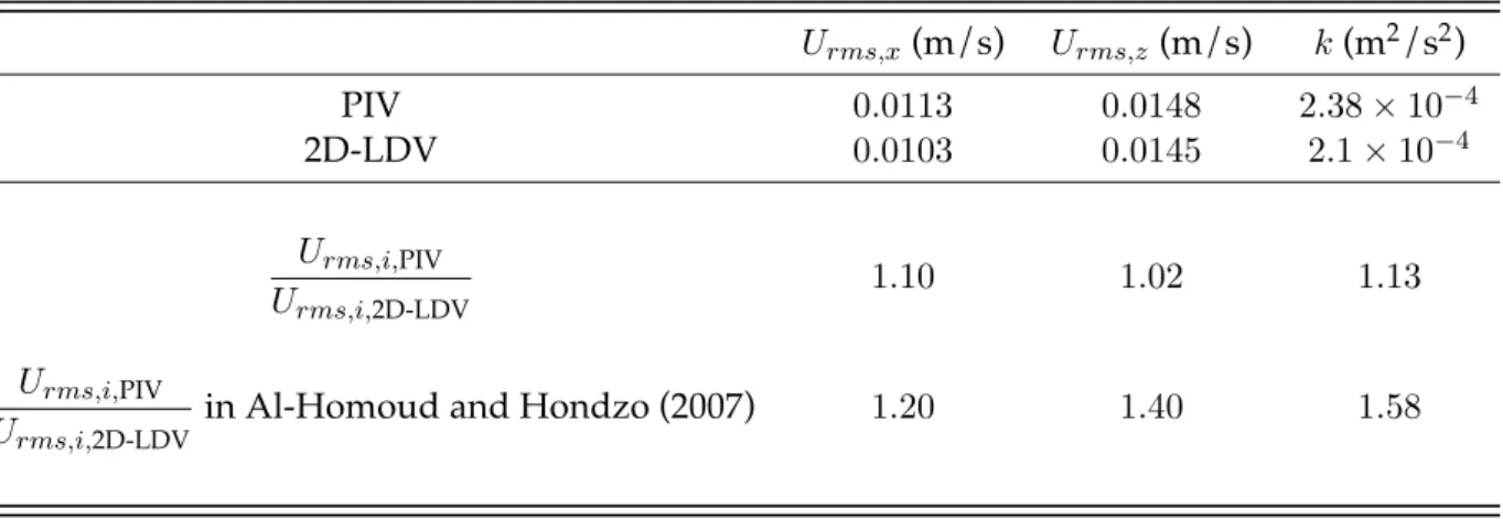
U_i′ Turbulent fluctuations of the fluid density around the mean . . . (m·s−1) U_i′U_j′ Reynolds stresses . . . (m2·s−2) Urms,i Turbulent intensity . . . .(m·s−1)

U_i(s) Fluid velocities seen by a solid body . . . (m·s−1) ul Characteristic velocity of the large turbulent eddies . . . (m·s−1)

us Characteristic velocity of the small turbulent eddies . . . (m·s−1)

V Vectorial particle velocity . . . (m·s−1₎

Vi Particle velocity along the ithdirection . . . (m·s−1)

Vol Total volume occupied by the particles and the fluid . . . (m3)

Vset Settling velocity for solid particles falling in stationary fluid . . . (m·s)

Wi Wiener process . . . (-)

Xi Position of a particle . . . (m)

Greek Symbols

αi Constants used in the exact integrator model . . . (-)

αx, αy Constants used used to correct the parallax of a camera . . . (pixels−1)

β A constant used in the exact integrator model . . . (-) βx, βy Constants used used to correct the parallax of a camera . . . .(mm·pixels−1)

∆ Stroke of the grid oscillation . . . (m) ∆t The time of one subinterval used to solve the Basset history force . . . (s)

ε Dissipation rate of the turbulent kinetic energy . . . (m2·s−3) η Free-surface elevation . . . (m)

Γi The stochastic integral of the solid particle velocity . . . (m·s−1)

γi The stochastic integral of the fluid velocity . . . (m·s−1)

λl Characteristic size of the large turbulent eddies . . . (m)

λs Characteristic size of the small turbulent eddies . . . (m)

ν Kinematic viscosity . . . (m2·s−1) νT Turbulent viscosity . . . .(m2·s−1)

Ω Volume of a solid body . . . .(m3₎

Ωa Volume of a disk representing an alga . . . (m3)

Ωf Volume fraction of particles . . . (–)

Ωs Volume of a sphere . . . (m3)

Φi The stochastic integral of the solid particle position . . . .(m)

ψi The derivative in the integral of the Basset history force . . . (m·s−2)

ψn The derivative ψiat time τn . . . (m·s−2)

ρf Fluid density . . . (kg·m−3)

ρs Solid body density . . . (kg·m−3)

ρs/f Ratio of the density between the solid particle and the surrounding fluid . . . (-)

NOMENCLATURE xxi

τn The time t minus n time steps ∆t . . . (s)

τpart The particle relaxation time . . . (s)

2

Chapter 1

Introduction

Le mouvement de corps dans un écoulement est un problème classique de mécanique des fluides. Son analyse est nécessaire, par exemple, pour le transport de sédiments le long du littoral, de bulles d’air dans un tuyau ou des aérosols relâchés par un combustible. Ces particules peuvent poser des problèmes de fonctionnement pour beaucoup d’industriels, et des questions environmentales capitales.

Ce mémoire se concentre sur le transport d’algues le long des côtes. Les modèles ex-istants pour ce type de problèmes reposent sur une approche biologique, où l’évolution d’une population d’algues est modélisée à long terme par l’apport de nutriments. Cepen-dant, pour la gestion d’une structure en bord de mer, il est important de connaître les réponses à court terme de ces algues à l’évolution d’un écoulement naturel déterminé par la marée.

Pour prendre en compte les spécificités d’un écoulement côtier il faut pouvoir mod-éliser les courants de marée, l’effet des vagues ainsi qu’une bathymétrie complexe. Ainsi il est proposé ici de coupler deux modèles ; un modèle eulérien de relativement grande échelle pour l’écoulement moyen et un modèle stochastique lagrangien de petite échelle pour le transport des algues.

Ce mémoire est divisé en sept chapitres. Premièrement le contexte motivant le be-soin de la thèse est expliqué (chapitre 2). Ensuite les bases de la mécanique des flu-ides nécessaires pour comprendre le modèle développé sont rappelées dans le chapitre 3. Vient ensuite une description des forces qui régissent le mouvement d’un corps dans un écoulement (chapitre 4). Pour modéliser ces forces il est nécessaire de connaître la vitesse du fluide à la position d’un corps. Le modèle utilisé est donc décrit dans le chapitre 5. Puis la résolution numérique est ensuite expliquée dans le chapitre 6. Les validations de ce modèle numérique sont ensuite réalisées à partir de deux expériences (chapitres 7 et 8). La première concerne le cas de particules relâchées dans une turbulence stationnaire, quasi-isotrope, générée par des grilles oscillantes, et la deuxième envisage des particules dans un canal partiellement obstrué. Fort de ces validations, le modèle est ensuite testé pour l’écoulement réel autour d’une centrale électrique en Normandie, dont les résultats préliminaires sont donnés dans le chapitre 9.

The presence of bodies in a flow and the transport patterns of these bodies is a classic problem in fluid mechanics. It’s analysis is required, whether it is for the transport of sediments along a coastline, the apparition of air bubbles in pipe flow or aerosols released by fossil fuels. It is important to develop tools predicting the motion of those particles, as they can hinder the operation of many industrial structures and affect severely the environment.

The focus of this thesis is on the transport of algae particles along a coastline, as it is a problem that has only been studied from a biological point of view. Typical algae transport model focus on the long term evolution of a population (or bloom) of algae by modelling the inflow of nutriments. However there is an industrial need to predict the short term response of such a population to flow variations due to tidal effects.

The aim of this thesis is therefore to present a model that will predict the transport of algae particles along the coastline. The environmental flow along a coastline has several specificities, including tidal currents, wave-breaking and a complex bathymetry, that need to be accounted for. These affect the flow on a large scale, however the motion of algae particles is also subject to smaller scale effects, such as the inertial properties of the algae, or the turbulence of the flow. In order to combine the large scale effects and the small scale effects efficiently, the transport of algae particles along the coastline is modelled through the coupling of two models. A relatively large scale Eulerian model is used to solve for the mean flow and a small scale Lagrangian stochastic particle model is used to predict the turbulent fluctuations of the flow and the transport of individual algae particles.

This thesis is divided into seven chapters. Firstly the context that led to a need for this research will be explained (chapter 2). Then the theoretical background of fluid mechanics necessary to understand to development of the model will be explained in chapter 3. Thirdly the forces acting on the motion of a particle transported by a flowing fluid will be described (chapter 4). A necessary requirement to predict the transport the motion of solid particles is to know the fluid velocity at the location of the particle, and therefore the model predicting the turbulent velocity at the location of a fluid particle will be explained in chapter 5. The combination of a fluid velocity and particle velocity model creates a complex model to solve numerically, and therefore the development and properties of such a model will be presented in chapter 6. This model will then be validated using two experiments (chapters 7 and 8). The first is for the case of particles released in quasi-isotropic grid generated stationary tur-bulence, and the second is for particles released in a partially obstructed channel. The model will then be applied and briefly analysed for the real flow around a nuclear power plant in Normandy (chapter 9).

6

Chapter 2

Context

Où le contexte de la problématique du transport d’algues en bord de mer est expliqué. Les côtes de Bretagne et Normandie sont sujettes à une augmentation du volume d’algues échouées. Ces algues, principalement de type Ulves, ne sont pas toxiques pour l’homme individuellement, mais les quantités échouées créent des problèmes lors du processus de décomposition. Ce phénomène, connu sous le nom de marées vertes, pose ainsi des prob-lèmes de gestion de ces côtes, en terme de propreté et sureté. Pour les industriels, les problèmes viennent du fait que ces algues bloquent partiellement l’accès à l’eau.

Pour répondre à ce problème une approche de modélisation mixte Eulérienne et La-grangienne est proposée. Dans cette approche un modèle Eulérien est utilisé pour simuler le courant moyen en traitant les mécanismes modélisés par les grandes échelles. Ensuite un modèle Lagrangien est utilisé pour suivre les trajectoires des algues dépendant de mé-canismes modélisés par des petites échelles.

Enfin, pour justifier l’approche de modélisation retenue, des nombres adimensionnels classiques sont utilisés. La fraction volumique des particules permet de prédire qu’un couplage fluide–eau sera suffisant pour les applications envisagées ici, et le nombre de Stokes des particules permet de justifier que les corps solides ne peuvent pas être con-sidérés comme de simples particules de fluide. Ensuite une description des modèles de transport d’algues est donnée. Cependant il existe peu de modèles permettant de mod-éliser le transport d’algues en bord de mer, et ceux-ci se concentrent principalement sur l’évolution d’une population d’algues. Or pour la problématique de la thèse, il faudrait pouvoir prédire la réponse d’un groupe d’algues aux variations de l’écoulement.

Ainsi, pour servir de référence, d’autres modèles de transport de particules dans un écoulement sont décrits, par exemple le transport d’aérosols dans l’atmosphère ou de bulles dans les canalisations.

2.1 The algae problematic

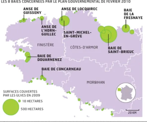
The coast of Normandy and Brittany in France have seen mass deposition of algal blooms, see for example figure 2.1.

Figure 2.1: Surface covered in Ulva in Brittany during the year 20091_{. The green circles represent}

surfaces covered with alga.

The reason why the regions of Brittany and Normandy are affected so severely are of two origins. Firstly there are geographical reasons. In large beaches, with a small slope, the effect of the waves (usually in combination with a small tidal current) might trap the algae close to the beach, where with a small water depth the algae will be in relatively warm water and have easy access to sunlight. Secondly there is the access to nutriments. The type of sediments and the proximity of these (i.e. in shallow water) can also increase the nutriments present in the water. Secondly during the summer the rivers have a smaller discharge, and therefore they reach the sea with a higher concentration of nutriments. Finally, with the human occupation along the coastline, rain water enters the ocean faster, and through human activity (such as agriculture) a higher dose of nutriments enters the water cycle. Further details on the reasons behind the increase of Ulva populations can be found in Inf’ODE (1999). Nonetheless these algae are not toxic in their natural form, but the amount that is deposited causes many problems. When deposited on the beach these algae will decompose, and because of the amount present, the fumes emitted from this decomposition prove to be hazardous. Furthermore the presence of these algal blooms in the water will partially block the access to sea water. This proves to be particularly cumbersome for harbours or industrial structures that requires readily available sea water in their manufacturing process.

The only modifications to the growth process of the algal blooms that can be undertaken are to the human factors. However a modification of the human activities will be very long, expensive and complex, and might only shift the problem to another type of algae. For this purpose, the objective

MODELLING APPROACH 8

of this thesis is to develop a model to predict the transport of algal particles in a coastal environment surrounding an industrial complex so that civil engineering solutions can be found to deviate these blooms from the point of interest until curative solutions can be developed to reduce the presence of algal blooms along the coast in the long run.

2.2 Modelling approach

The model developed in this thesis will aim to predict the short term response of macro algae to a change in the flow along the coast, such as during on tide. This is done to provide a tool that can be used to protect industrial structures that require sea water in their manufacturing process from clogging due to algal bloom. Due to the fairly short term response of this problematic some parameters such as the growth and decay of an algal bloom can be ignored, however this requires a good modelling of the flow.

To model accurately the coastal flow around an industrial structure during a time scale of several hours (a tide cycle) several large scale characteristics of the flow need to be taken into account. For example the effects of the bathymetry, of the tides and the wave induced current will need to be considered. However the motion of an individual alga in the flow depends also on smaller scale effects, such as the physical characteristics of the body and the turbulence generated by the flow. To be able to include all the physical processes occurring over different spatial and temporal scales a mixed Eulerian and Lagrangian approach has been adopted. An Eulerian model will be used to solve for the mean fluid velocities over a large area in order to deal with all the large scale processes. These velocities will then be inputed in a Lagrangian model following the path of individual algae particles. This Lagrangian model will deal with all the smaller scale processes. A mixed Eulerian and Lagrangian approach allows also future developments to be added easily on the model to include further parameters that affect individual alga particles, such as a change of density or even the death of individual algae.

2.3 Categorising the problem

For the problem at hand we saw that looking purely at the scales of physical processes involved, the problematic needs to consider a wide range of motions. Large scales are necessary to predict accurately the environmental flow of the algae problem and small scales to consider the inertial effects of individual algae particles. Poelma et al. (2007) gives an overview of parameters that can be used to categorise a particle laden flows. Considering this approach the non-dimensional number Ωf, which

represents the volume fraction of particles as introduced by Elghobashi (2006), will be considered:

Ωf =

NrΩ

Vol (2.1)

Nr is the number of particles present in the flow, Ω is the volume occupied by a single particle and

Vol is the total volume occupied by the particles and the fluid. Elghobashi (2006) showed that for

volume fraction of particles smaller than 10−6 _{a one way fluid–particle coupling can be done. A one}

way fluid–particle coupling means that the information from the fluid is given to the particle motion, but there is no transfer of information from the particles to the fluid flow. A quick calculation shows that a volume fraction of 10−6_{can correspond to the case of algae that can potentially cover a surface}

100× 1 m2and a millimetre thick transported in a volume of fluid 500× 100 × 2 m3, which is typical for the transport of algae.

Fessler (1994): St =τp τs (2.2a) τp= (2ρs+ ρf) D2 36νρf (2.2b) τs= (_ν ε )1 2 (2.2c)

Where ρsis the particle density (the “s” stands here for “solid”), ρf is the fluid density, D is a

char-acteristic length of the body, ν is the kinematic viscosity and ε is the dissipation rate of the turbulent kinetic energy. This Stokes number can be considered as the relationship between two characteristic times. τpwhich is the relaxation time for a particle experiencing only Stokes drag, and τswhich is the

characteristic time for the small turbulent eddies. Eaton and Fessler (1994) show that particle with a Stokes number between 0.01 and 25 can be considered to be partially affected by the motion of the fluid. For alga particles such as those described in section 9.1 transported in a typical environmental with a dissipation rate of the order 10−5_m2_·s−3_{this gives Stokes number ranging from 1-30. We will}

analyse these characteristic time scales and dimensionless numbers, amongst others, in chapter 7. Therefore the parameter Ωf shows that the model developed in this thesis can assume that the

par-ticles will not affect the flow, which simplifies the use of a Lagrangian model on top of an Eulerian model. The parameter St shows that the particles will not affect the flow and therefore that small scale effects cannot be ignored. These effects can be easily calculated within a Lagrangian model.

2.4 Existing algae transport models

In literature the only models that deal with the transport of algae particles have approached the prob-lem from a biological point of view. These models focus more the growth and decay of a population of algae within an bay or a lagoon. This therefore requires a model that will cover several kilometres and several weeks of simulations.

If one ignores the articles that focus on the nutrients that affects the population of algae in a body of water there are some articles that try to relate the evolution of a population of algae in relation to hydraulic properties. Biber (2007) has done a study of algae in the Biscayne Bay, in Florida, USA. In this study the author records the amount of Sargassum and Red algae entering and leaving the bay, and finds that these algae enter the bay during flood and leave the bay during ebb. The author also finds that during different periods of the year these volumes are not the same.

In Bosence (1976) a study is done on the presence of algae in Mannin Bay, in Ireland. In this study the author tries to link the presence of coralline algae at different location in the bay to the direction and strength of the currents, the distribution and orientation of wave ripples as well as the bathymetry and bed type.

In Flindt et al. (2007) the study goes slightly further as here the authors try to link an average algae velocity to an average current velocity. This is done for four kind of algae: Ulva, Chaetomorpha, Ceramium and Cladophora species. The authors than go to calculate the mean settling rates for these algae.

As can be found from these three articles, there hasn’t been an in depth study of the hydrodynamic and physical properties that will govern the motion of algae particles. Nonetheless some numerical models exist. These models often use water quality models to transport nutrients that will affect the growth and decay of a population of algae. These models can be found for example in Solidoro

et al. (1997) which focus on the evolution of the population of Ulva rigida in the Venice lagoon (Italy)

EXISTING PARTICLE TRANSPORT MODELS 10

macro algae (defined through its growth parameters) in the Rio de Aveiro bay (Portugal) during 6 consecutive years.

The two most interesting algae transport models present in literature are those that use the coastal current to transport particles in order to affect the growth of algae. Donaghay and Osborn (1997) for example consider micro algae, such as Aureococcus anophagefferens, in terms of concentrations of this specific pollutant, and because of their size it is assumed that these algae follow exactly the fluid velocities, upon which is added growth and decay model. Salomonsen et al. (1999) use also a growth and decay model, but for a macro alga (Ulva lactuca). On top this model is an erosion and sedimentation model to define when algae will be carried by following the current calculated by a hydrodynamic model. This model is then applied to Møllekrogen bay in Denmark, which is typically 10- 100 km2, and has a simulation done over several days (up to a month).

Nonetheless these existing models prove to be ineffective for the problematic at hand, and inspiration should be found in particle transport models for other kind of particles.

2.5 Existing particle transport models

Models describing the motion of particles in a fluid have been studied for many years. For example Einstein in 1905 presented a model describing Brownian motion, where summary and translation of this article can be found in Gardiner (2004) and a short description of Brownian motion can be found in section 5.1. For the problem at hand, the trajectories of a group of algae needs to be modelled so that the effectiveness of civil engineering works to protect industrial structures or harbours from the accumulation of algae can be tested. The models presented in this section are, for the most part, mixed Eulerian and Lagrangian models. The amount of information treated, as well as the scales of the simulations, will also be given.

Models such as the ones presented in Monti and Leuzzi (2010), Issa et al. (2009), Heemink (1990) or Stijnen et al. (2006) predict the motion of particles in environmental flows by adding to the mean flow an estimation of the diffusion due to turbulence. These models focus on a smaller scale of motion, typically 10 m - 1 km and 1 - 24 h, but still large enough to model the specificities of environmental flows such as tides, waves, turbulent diffusion and the effect of bathymetry. However the turbulence is predicted simply, through the use of a diffusion constant (which represents the turbulence), and none of the physical characteristics of the bodies are taken into account.

To find models that consider the physical properties of bodies one needs to look at models used to predict the transport of aerosols or bubbles. Example of aerosol models, which are models that con-sider solid particles interacting with a gas can be found in Csanady (1963), Minier and Peirano (2001) or Sawford and Guest (1991). Yeo et al. (2010) is a good example of a bubble model, which is a model with distinct gas particles transported in a fluid. These models are developed for small particles with a large density difference with the surrounding fluid. The algae particles are large in comparison to these models, and have a very small difference in density with the surrounding fluid. Furthermore these models typically require more information on the flow than is generally available in environ-mental flow modelling (see chapter 3) and therefore tend to be applicable for a smaller scale of fluid models (because of computing power).

It is also possible to consider larger particles in the flow with Direct Numerical Simulations, in Uhl-mann (2008) for example, but these models can only be used for a very small scale of simulation.

12

Chapter 3

Environmental Flow Modelling

Où les bases de la mécanique des fluides sont rappelées. Dans la première partie de ce chapitre, la différentiation entre les modèles de type Eulérien et Lagrangien est expliquée. Ensuite les équations de Navier-Stokes sont introduites, ainsi que l’équation de continu-ité. Enfin il est ensuite expliqué comment obtenir les équations de Saint-Venant, qui sont souvent utilisées pour modéliser les écoulements côtiers. La seconde partie introduit la modélisation de la turbulence. Cela commence par l’introduction du nombre de Reynolds, ainsi que la décomposition de la vitesse du fluide qui permet d’obtenir les contraintes de Reynolds. Il est ensuite expliqué comment modéliser ces contraintes à travers deux types de modèles. Les modèles de type viscosité turbulente, avec la mise en avant du modèle k-ε, et les modèles suivant l’évolution dans le temps de ces contraintes. Finalement, les hypothèses de Kolmogorov sont introduites ainsi que les grandeurs caractéristiques qui en découlent.

3.1 General principles of fluid mechanics

Before going more in depth into the model describing the transport of algae particles in coastal water there are a few general principles of fluid mechanics which need to be understood. Firstly there are two different general methods used to describe a flow of fluid. One focuses on individual fluid particles (or individual bundles of fluid particles) and follows them in time. This type of methods are called Lagrangian methods. The second method focus on the behaviour of the fluid within an area. These methods are called Eulerian.

Lagrangian methods can become very time consuming and complex when a large volume of fluid is observed and therefore when modelling the flows Eulerian method are usually preferred. When it comes to environmental flows there are two different flow models which are commonly used. These environmental flows, which are the water flows of interest for the problem considered in this thesis, are considered to be Newtonian, which means that their viscosity (represented with the symbol µ, or if divided by the fluid density ν ) which is a measure of their resistance to deformations caused by shear or tensile stresses, is constant. They are also considered incompressible, which means that they have a constant density (represented with the symbol ρf).

The first model described, which is the basis for all fluid models which are considered Newtonians, is the Navier-Stokes equation of motion. This equation is found by applying newton’s second law of motion (conservation of momentum) to an area of the fluid. In its incompressible form it is given by the following equation (Viollet et al., 2002):

∂U

∂t +U· ∇U = −

1

ρf∇P + g + ν∇

2_{U (3.1)}

In this equation the symbol U represents the fluid velocity, P is the fluid pressure,∇ is the gradient

operator, g is the vectorial representation of the acceleration due to gravity and∇2_{is the Laplacian}

op-erator. Equation 3.1 is written in its vectorial form, where the symbols in bold show vectors. However there are two other form of notations which can be used, and will be introduced here as they will be used later on in the thesis. The Cartesian (x,y,z) projection of the vectorial form of the Navier-Stokes equation is given by:

∂Ux ∂t + Ux ∂Ux ∂x + Uy ∂Ux ∂y + Uz ∂Ux ∂z =− 1 ρf ∂P ∂x + ν ( ∂2Ux ∂x2 + ∂2Ux ∂y2 + ∂2Ux ∂z2 ) (3.2a) ∂Uy ∂t + Ux ∂Uy ∂x + Uy ∂Uy ∂y + Uz ∂Uy ∂z =− 1 ρf ∂P ∂y + ν ( ∂2Uy ∂x2 + ∂2Uy ∂y2 + ∂2Uy ∂z2 ) (3.2b) ∂Uz ∂t + Ux ∂Uz ∂x + Uy ∂Uz ∂y + Uz ∂Uz ∂z =− 1 ρf ∂P ∂z − g + ν ( ∂2Uz ∂x2 + ∂2Uz ∂y2 + ∂2Uz ∂z2 ) (3.2c)

Note that in this case the vertical axis is assumed to be orientated in the upward direction. Finally equation 3.1 can be written following the Einstein notations

∂Ui ∂t + Uj ∂Ui ∂xj =− 1 ρf ∂P ∂xi + gi+ ν ∂2Ui ∂x2_j (3.3)

Where the subscript i represents the direction of the flow considered, all the subsequent subscripts that are used j or later on k represent a summation over the components of direction.

Furthermore the Navier-Stokes equations need to include the continuity equation, which in incom-pressible flows is given by (Viollet et al., 2002):

GENERAL PRINCIPLES OF TURBULENCE MODELLING - FIRST-ORDER MODELS 14 ∂Ux ∂x + ∂Uy ∂y + ∂Uz ∂z =0 (3.4)

The continuity equation ensures that in within the volume of measurement, in the absence of a source or a sink of fluid, no fluid will be lost or created.

The second flow model commonly used in environmental problems are the non-linear Shallow Water equations. These are often used in free-surface flows and they can be obtained by integrating the Navier-Stokes equations over the depth of the flow under the hypothesis that horizontal length scale is much greater than the vertical length scale, and that the vertical velocity components are negligible. In its conservative form the Shallow Water equations are given by (Viollet et al., 2002):

∂Ui ∂t + Uj ∂Ui ∂xj =−g∂η ∂xi + ν h ∂ ∂xj [ h ( ∂Ui ∂xj + ∂Uj ∂xi )] (3.5)

With η representing the free-surface elevation from the mean elevation and h the depth of the fluid and all the velocity values given here are depth-averaged. For the non-linear Shallow Water equations the continuity equation is given by (Viollet et al., 2002):

∂h ∂t + ∂hUx ∂x + ∂hUy ∂y =0 (3.6)

Again the velocity values are depth-averaged.

These models are applied over a domain of interest, and therefore it is necessary to know the be-haviour of the flow along the boundaries. This is known as the boundary conditions. For the bound-ary conditions on the Navier-Stokes equations see Viollet et al. (2002), and for the boundbound-ary conditions on the non-linear Shallow Water equations see Hervouet (2007). A more sophisticated set of shallow water equations will be presented later on in chapter 9.

3.2 General principles of turbulence modelling - first-order models

During the observation of most real flows it is possible to observe eddies of different size, shape and direction. These eddies create a fluctuation around the mean flow velocities in a process called turbulence. The intensity of the turbulence is usually characterised through a dimensionless number called the Reynolds number (Viollet et al., 2002):

Re = U d

ν (3.7)

The Reynolds number is the ratio between a characteristic fluid velocity U, a characteristic flow length

dand the kinematic viscocity ν. The flow is generally considered to be laminar (which means that

there are virtually no turbulent fluctuations) for low values of the Reynolds number (typically under 2300). Above this value small perturbations will be amplified to reach a finite value. From this defini-tion of turbulence, Reynolds introduced a decomposidefini-tion of the fluid velocity given by the following equation (Viollet et al., 2002):

Where Ui represents the mean fluid velocity (in the turbulent sense, it should not be confused with

the depth-averaged velocities found through the Shallow Water equations) and U′

i represents the

fluctuations around this mean value. This decomposition can be applied to other fluid quantities, such as the pressure. Figure 3.1 shows a schematic description of this concept.

... U_i′ . Ui . 0.2 . 0.3 . 0.4 . 0.5 . 0.6 . 0.7 . 0.8 . 0 . 0.02 . 0.04 . 0.06 . 0.08 . 0.1 . 0.12 . t(s) . U (m / s )

Figure 3.1: An example of a recording of a turbulent fluid velocity in time taken from velocity mea-surements of the experiment in section 8.2.

The Reynolds decomposition introduced in equation 3.8 can be used to rewrite the Navier-Stokes and the continuity equations (equations 3.3 and 3.4). Averaging these new equations we get the Reynolds equations (Pope, 2000): ∂Ui ∂xi =0 (3.9a) ∂Ui ∂t + Uj ∂Ui ∂xj =− 1 ρf ∂P ∂xi + gi+ ν ∂2Ui ∂x2_j − ∂ ∂xj ( U_i′U_j′ ) (3.9b) The terms U′

iUj′ are known as the Reynolds stresses, and they represent the momentum transfer by

the turbulent fluctuations. Due to these stresses the Reynolds equations are unclosed, and from this closure problem comes all the modelling of the turbulence. This tensor is symmetrical (U′

iUj′ = Uj′Ui′)

and the diagonal components (U′

iUi′) are normal stresses whereas the off diagonal components are

shear stresses. The simplest method to model the Reynolds stresses is to consider that they act as vis-cous stresses, since turbulent eddies are responsible for mixing and energy dissipation. Therefore an artificial viscosity called the turbulent (or eddy) viscosity νT will be introduced. Using Boussinesq’s

assumption that the Reynolds stresses are proportional to the mean rates of strain (Pope, 2000) gives:

−U′

iUj′ =2νTSij −

2

3kδij (3.10)

Where Sij is the mean rate of strain tensor is:

Sij = Sji = 1 2 ( ∂Ui ∂xj +∂Uj ∂xi ) (3.11)

GENERAL PRINCIPLES OF TURBULENCE MODELLING - FIRST-ORDER MODELS 16

The symbol k is the turbulent kinetic energy (TKE), which is the kinetic energy of the fluctuating part of the flow per unit mass. It is defined by:

k = 1

2U

′

iUi′ (3.12)

Using this, the Reynolds averaged Navier-Stokes equation (3.9b) can be rewritten as:

∂Ui ∂t + Uj ∂Ui ∂xj =− 1 ρf ∂ ∂xi ( P +2 3ρfk ) + gi+ ∂ ∂xj [ (ν + νT) ∂Ui ∂xj ] (3.13)

The term 2ρfk/3is often considered negligible compared to P .

The simplest way to consider the turbulent viscosity is to assume a constant value throughout the domain, and in many real applications this can be sufficient to obtain an estimation of the mean fluid velocities, however if one is interested in the diffusive abilities of the flow, a more detailed model of the for this viscosity is required. A commonly used model is the k-ε model developed by Jones and Launder (1972). To obtain a model for the turbulent kinetic energy this model starts by subtracting the Reynolds equations from the Navier-Stokes equations. This gives the evolution of the fluctuating velocities: ∂U_i′ ∂t + Uj ∂U_i′ ∂xj =− U_j′∂Ui ∂xj + ∂ ∂xj ( U_i′U_j′ ) + ν∂ 2_U′ i ∂x2 j − 1 ρf ∂P′ ∂xi (3.14)

Therefore, from equations 3.14 and 3.12 it is possible to obtain the evolution of the turbulent kinetic energy: ∂k ∂t + Uj ∂k ∂xj =−U_i′U_j′∂Ui ∂xj − ∂ ∂xk ( 1 2Ui′Uj′Uj′ + U_i′P′ ρf − 2νU ′ jsij ) − 2νsijsij (3.15)

Where sij is the fluctuating rate of strain tensor given by:

sij = 1 2 ( ∂U_i′ ∂xj +∂U ′ j ∂xi ) (3.16)

Equation 3.15 can be rewritten to make visible certain characteristics.

∂k ∂t + Uj ∂k ∂xj =P − ∂T ′ j ∂xj − ε (3.17)

The symbolP corresponds to the production of turbulent energy and it is given by:

P = − U′ iUj′

∂Ui

∂xj

The notation Sij can be used in place of the velocity gradient because of the symmetrical nature of

the Reynolds stresses and of Sij. The symbol Ti′corresponds to the flux of turbulent energy and it is

given by: T_i′= 1 2U ′ iUj′Uj′ + U_i′P′ ρf − 2νU ′ jsij (3.19)

And ε is the dissipation of turbulent energy defined by:

ε = 2νsijsij (3.20)

The terms to be closed in of equation 3.17 are the flux of the turbulent kinetic energy T′

i and the

dissipation rate of the turbulent kinetic energy ε. Using Boussinesq’s assumption on Reynolds stresses (equation 3.10) the productionP is given as:

P = − ( 2 3kδij− 2νTSij ) Sij =2νTS2 (3.21)

In this calculation, we used the property Sijδij = Sii= 0and the scalar mean rate of strainS is defined

as:

S =√2SijSij (3.22)

And therefore the production term is known. In the k-ε model the flux of turbulent kinetic energy is modelled as a diffusion gradient:

T_i′ =−νT

σk

∂k

∂xi (3.23)

Note that the turbulent damping coefficient σkis a scalar (where the subscript k is a standard notation,

and not a vectorial component) generally taken equal to 1. The turbulent viscosity is specified by the following dimensional equation:

νT = Cµ

k2

ε (3.24)

With Cµbeing a constant, experimentally found to be 0.09. The evolution of turbulent kinetic energy

(equation 3.17) can therefore be simplified to:

∂k ∂t + Uj ∂k ∂xj =P + ∂ ∂xj ( νT σk ∂k ∂xj ) − ε (3.25)

The k-ε model chooses to model the dissipation rate instead of using the definition 3.20. ε can be con-sidered as the turbulent energy flow rate in the energy cascade (see later in this section), determined

GENERAL PRINCIPLES OF TURBULENCE MODELLING - FIRST-ORDER MODELS 18

by the large scales of turbulence and assumed to be independent of the viscosity (which is true at high Reynolds numbers). It can therefore be modelled by the heuristic equation:

∂ε ∂t + Uj ∂ε ∂xj = Cε1Pε k + ∂ ∂xj ( νT σε ∂ε ∂xj ) − Cε2 ε2 k (3.26)

The constant of the k-ε model are set as Cε1 = 1.44, Cε2 = 1.92, σk = 1.0and σε = 1.3(Launder and

Sharma, 1974).

Naturally the turbulence models can also be applied to the Shallow Water equations. Integrating equation 3.13 over the vertical gives:

∂Ui ∂t + Uj ∂Ui ∂xj =−g∂η ∂xi +ν h ∂ ∂xj [ h ( ∂Ui ∂xj +∂Uj ∂xi )] −1 h ∂ ∂xj ( hU_i′U_j′ ) (3.27)

The turbulent fluctuations of free-surface and of the water depth are assumed to be negligible due to the action of gravity. The shallow water equations can also be written using the turbulent viscosity hypothesis: ∂Ui ∂t + Uj ∂Ui ∂xj =−g∂η ∂xi + 1 h ∂ ∂xj [ h (ν + νT) ( ∂Ui ∂xj +∂Uj ∂xi )] (3.28)

Where all the fluid velocity values are still depth-averaged. The k-ε equations can also be written in a depth-averaged version. These equations are similar to equations 3.25 and 3.26, but with added terms resulting from the depth-averaging (Rodi, 2000):

∂k ∂t + Uj ∂k ∂xj =P + ∂ ∂xi ( νT σk ∂k ∂xi ) − ε + Pk (3.29a) ∂ε ∂t + Uj ∂ε ∂xj =Cε1Pε k + ∂ ∂xi ( νT σε ∂ε ∂xi ) − Cε2 ε2 k + Pε (3.29b)

The two additional terms Pkand Pεare given by:

Pk= u2_∗|U| h (3.30a) Pε=CεCε2 √ Cµu5_∗|U|3 h2 (3.30b)

The constants in equations 3.29 and 3.30 are set to: Cε1 = 1.44, Cε2 = 1.92, Cε = 3.6, Cµ = 0.09,

σk = 1.0and σε = 1.3in Launder and Sharma (1974) and Rodi (2000). Equations 3.29 are then used

in equations 3.28 through the usual relation:

νT = Cµ

k2

3.3 General principles of turbulence modelling - second-order models

∂ ∂t ( U_i′U_j′ ) + Uj ∂ ∂xj ( U_i′U_j′ ) =Pij +Rij− ∂ ∂xk Tkij − εij (3.32)

WherePij is the production tensor and it is defined as:

Pij ≡ −U_j′U_k′ ∂Ui ∂xk − U′ iUk′ ∂Uj ∂xk (3.33)

Rij is the pressure rate of strain tensor and it is defined as:

Rij ≡ P′ ρf ( ∂U_i′ ∂xk +∂U ′ j ∂xk ) (3.34)

And εij is the dissipation tensor, defined by:

εij ≡ 2ν

∂U_i′ ∂xk

∂U_j′

∂xk (3.35)

Tkij are the Reynolds stress flux which are defined by:

Tkij =T (u) kij + T (P ) kij + T (ν) kij (3.36a)

T_kij(u) ≡U_i′U_j′U_k′ (3.36b)

T_kij(P )≡ 1 ρf U_i′P′δjk+ 1 ρf U_j′P′δik (3.36c) T_kij(ν)≡ − ν∂U ′ iUj′ ∂xk (3.36d)

Now that the evolution of the Reynolds stresses are known models are required to provide closure to the Reynolds stress flux, the dissipation and the pressure rate of strain tensor. Pope (2000) gives a thorough overview of such models. We will now consider the simplest one.

For high Reynolds numbers because of local isotropy (see the Kolmogorov hypotheses described later on) the dissipation can be rewritten as:

εij =

2

3εδij (3.37)

Rotta’s model is often used to close the pressure rate of strain tensor (equation 3.34). To describe this model it is necessary to be aware that the fluctuating pressure field can be decomposed into three contributions, taken from the observation of the Poisson equation for fluctuating pressure (Pope, 2000):

GENERAL PRINCIPLES OF TURBULENCE MODELLING - SECOND-ORDER MODELS 20

P′ = P(r)+ P(s)+ P(h) (3.38)

The first contribution P(r)_{is known as the rapid pressure as it responds immediately to a change of}

the mean velocity gradients. It is defined through the following relation:

1 ρf∇ 2_P(r)_{=− 2}∂Ui ∂xj ∂Uj ∂xi (3.39)

The second contribution is known as the slow pressure, because it takes longer than P(r)_{to respond}

to mean velocity gradients, and it is defined by:

1 ρf∇ 2_P(s)₌₋ ∂2 ∂xi∂xj ( U_i′U_j′ − U_i′U_j′ ) (3.40)

The final contribution is the harmonic pressure, which is used to impose the boundary conditions. It is given by the following equation:

1

ρf∇

2_P(h)_{=0 (3.41)}

These definitions can be used to decompose the pressure rate of strain tensor (equation 3.34):

Rij =R(r)ij +R (s) ij +R (h) ij (3.42a) R(r) ij = P(r) ρf ( ∂U_i′ ∂xk +∂U ′ j ∂xk ) (3.42b) R(s) ij = P(s) ρf ( ∂U_i′ ∂xk + ∂U ′ j ∂xk ) (3.42c) R(h) ij = P(h) ρf ( ∂U_i′ ∂xk +∂U ′ j ∂xk ) (3.42d)

Rotta’s model was developed in a scenario where only the slow pressure rate of strain tensor con-tributes to the Reynolds stresses. In decaying homogeneous anisotropic turbulence there are no pro-duction or transport of those stresses so that the exact Reynolds stress equation (3.32) becomes:

d dt ( U_i′U_j′ ) =R(s)_ij − εij (3.43)

The anisotropy of the flow can be quantified using the following anisotropy tensor:

bij =

U_i′U_j′

2k − 1

3δij (3.44)

In this case the evolution of the anisotropy tensor can be found using equations 3.43, 3.15 (with neg-ligible production or fluxes) and the isotropic turbulent dissipation rate (3.37):