arXiv:1503.02062v3 [math.PR] 12 Jun 2015
Utility maximization with random horizon: a BSDE approach
Monique Jeanblanc
1Thibaut Mastrolia
3Université d’Evry Val d’Essonne2
Université Paris Dauphine4
LaMME, UMR CNRS 8071 CEREMADE UMR CNRS 7534
[email protected] [email protected]
Dylan Possamaï
Anthony Réveillac
Université Paris Dauphine4
INSA de Toulouse5
CEREMADE UMR CNRS 7534 IMT UMR CNRS 5219
[email protected] Université de Toulouse
Abstract
In this paper we study a utility maximization problem with random horizon and reduce it to the analysis of a specific BSDE, which we call BSDE with singular coefficients, when the support of the default time is assumed to be bounded. We prove existence and uniqueness of the solution for the equation under interest. Our results are illustrated by numerical simulations.
Key words: quadratic BSDEs, enlargement of filtration, credit risk.
AMS 2010 subject classification: Primary: 60H10, 91G40; Secondary: 91B16, 91G60, 93E20, 60H20.
1
Introduction
In recent years, the notion of risk in financial modeling has received a growing interest. One of the most popular direction so far is given by model uncertainty where the param-eters of the stochastic processes driving the financial market are assumed to be unknown (usually referred as drift or volatility uncertainty). Another source of risk consists in an exogenous process which brings uncertainty on the market or on the economy. This kind of situation fits, for instance, in the credit risk theory. As an example, consider an investor who may not be allowed to trade on the market after the realization of some random event, at a random time τ , which is thought to be unpredictable and external to the market. In that context τ is seen as the time of a shock that affects the market or the agent. More precisely, assume that an agent initially aims at maximizing her expected utility on a given financial market during a periodr0, T s, where T ą 0 is a fixed deter-ministic maturi ty. However, she may not have access to the market after the random 1
The research of Monique Jeanblanc is supported by Chaire Markets in transition, French Banking Fed-eration.
2
Laboratoire de Mathématiques et Modélisation d’Évry (LaMME), Université d’Évry-Val-d’Essonne, UMR CNRS 8071, IBGBI, 23 Boulevard de France, 91037 Evry Cedex, France
3
Thibaut Mastrolia is grateful to Région Ile de France for financial support and acknowledges INSA de Toulouse for its warm hospitality.
4
Place du Maréchal de Lattre de Tassigny, 75775 Paris Cedex 16, France
5
time τ . In that context we think of τ as a death time, either for the agent herself, or for the market (or a specific component of it) she is currently investing in. Though very little studied in the literature, our conviction is that such an assumption can be quite relevant in practice. Indeed, for instance many life-insurance type markets consists of products with very long maturities (up to 95 years for universal life policies and to 120 years for whole life maturity). It is therefore reasonable to consider that during such a period of time an agent in age of investing money in the market will die with probability 1. Another example is given by markets whose maximal lifetime is finite and known at the beginning of the investment period, like for instance carbon emission markets in the United States.
Mathematically, while her original problem writes down as sup
πPA
ErU pXπ
Tqs, (1.1)
with A the set of admissible strategies π for the agent with associated wealth process Xπ
and where U is a utility function which models her preferences, due to the risk associated with the presence of τ , her optimization program actually has to be formulated as
sup
πPA
ErU pXπ
T^τqs, (1.2)
which falls into the class ofa priori more complicated stochastic control problems with random horizon.
The main approach to tackle (1.2) consists in rewriting it as a utility maximization problem with deterministic horizon of the form (1.1), but with an additional consumption component using the following decomposition from [10] that we recall:
sup πPA ErU pXπ T^τqs “ sup πPA E «żT 0 UpXπ uqdFu` U pXTπqp1 ´ FTq ff ,
with Ft:“ Pp τ ď t| Ftq and F :“ pFtqtPr0,T sbeing the underlying filtration on the market.
This direction was first followed in [22] when τ is a F-stopping time, then in [6] and in [7] if τ is a general random time. In all these papers, the convex duality theory (see e.g. [5] and [21]) is exploited to prove the existence of an optimal strategy. However, this approach does not provide a characterization of either the optimal strategy or of the value function (note that in [6] a dynamic programming equation can be derived if one assumes that F is deterministic and U is a Constant Relative Risk Aversion (CRRA) utility function). Another route is to adapt to the random horizon setting the, by now well-known, methodology in which one reduces the analysis of a stochastic control problem with fixed deterministic horizon to the one of a Backward Stochastic Differential Equation (BSDE) as in [16, 29]. This program has been successfully carried out in [24] in which Problem (1.2) has been proved to be equivalent to solving a BSDE with random horizon of the form Yt“ 0 ´ żT^τ t^τ Zs¨ dWs´ żT^τ t^τ UsdHs´ żT^τ t^τ fps, Ys, Zs, Usqds, t P r0, T s, (1.3)
in the context of mean-variance hedging, with Hs:“ 1τďsand W a standard Brownian
motion. The interesting feature here lies in the fact that under some assumptions on the market, the solution triplet pY, Z, U q to the previous BSDE is completely described in terms of the one of a BSDE with deterministic finite horizon. More precisely, if we assume that F is the natural filtration of W and if τ is a random time which is not a F-stopping time, then the BSDE with deterministic horizon associated with BSDE (1.3) is of the form Ytb“ 0 ´ żT t Zsb¨ dWs´ żT t fbps, Yb s, Zsbqds, t P r0, T s, (1.4)
with fb related to τ through a predictable process λ (see Section 2.2 for a precise
state-ment on this relationship). The usual hypothesis, for instance in credit risk modeling, is to assume λ to be bounded (as in [24]). This assumption, which looks pretty harmless, leads in fact to several consequences both on the modeling of the problem and on the analysis required to solve Equation (1.3). Indeed, λ is bounded implies that the support1
of τ is unbounded. As a consequence, the probability of the eventtτ ą T u is positive. Hence it does not take into account the situation where τ is smaller than T with prob-ability one. Note that from the very definition of (1.2), assuming τ to have a bounded or an unbounded support leads to two different economic problems: if the support is unbounded, with positive probability the agent will be able to invest on the market up to time T , whereas if τ is known to be smaller than T with probability one, the agent knows she will not have access to the market on the whole time intervalr0, T s.
The main goal of this paper is to solve (1.2) when the support of τ is assumed to be a bounded interval in r0, T s. As explained in the previous paragraph, this assumption leads to the unboundedness of λ. More precisely, it generates a singularity in Equation (1.3) (or in (1.4)) as λ is integrable on any intervalr0, ts with t ă T , and is not integrable onr0, T s. This drives one to study a new class of BSDEs, named as BSDEs with singular driver according to [18], which requires a specific analysis. We stress that the study of the BSDE of interest of the form (1.4) with fb to be specified later is not contained
in [18], and hence calls for new developments presented in this paper. Incidentally, we propose a unified theory which covers both cases of bounded and unbounded support for τ (see ConditionspH2q, pH2’q for a precise statement).
The rest of this paper is organized as follows. In the next section we provide some preliminaries and notations and make precise the maximization problem under interest. Then in Section 3, we extend the results of [16, 24] allowing to reduce the maximization problem with exponential utility to the study of a Brownian BSDE. The analysis of this equation is done in Section 4. To illustrate our findings, and to compare problems of the form (1.1) and (1.2), we collect in Section 5 numerical simulations together with some discussion.
Notations: Let N˚:“ Nzt0u and let R`be the set of real positive numbers. Throughout
this paper, for every p-dimensional vector b with p P N˚, we denote by b1, . . . , bp its
coordinates and for α, βP Rpwe denote by α¨ β the usual inner product, with associated
norm }¨}, which we simplify to | ¨ | when p is equal to 1. For any pl, cq P N˚ ˆ N˚,
Ml,cpRq will denote the space of l ˆ c matrices with real entries. When l “ c, we let
MlpRq :“ Ml,lpRq. For any M P Ml,cpRq, MT will denote the usual transpose of M .
For any xP Rp, diagpxq P M
ppRq will stand for the matrix whose diagonal is x and for
which off-diagonal terms are 0, and Ip will be the identity of MppRq. In this pape r
the integralsştswill stand for şpt,ss. For any dě 1 and for any Borel measurable subset I Ă Rd, BpIq will denote the Borel σ-algebra on I. Finally, we set for any p P N˚, for
any closed subset C of Rpand for any aP Rp
distCpaq :“ min
bPCt}a ´ b}u,
and
ΠCpaq :“ tb P Ctpωq, }a ´ b} “ distCpaqu .
2
Preliminaries
2.1
The utility maximization problem
Set T a fixed deterministic positive maturity. Let W “ pWtqtPr0,T s be a d-dimensional
Brownian motion (dě 1) defined on a filtered probability space pΩ, GT, F, Pq, where F :“
pFtqtPr0,T sdenotes the natural completed filtration of W , satisfying theusual conditions.
1
GT is a given σ-field which strictly contains FT and which will be specified later. Unless
otherwise stated, all equalities between random variables onpΩ, GTq are to be understood
to hold P´ a.s., and all equalities between processes are to be understood to hold Pb dt ´ a.e. (and are as usual extended to hold for every t ě 0, P ´ a.s. if the considered processes have trajectories which are, P´ a.s., càdlàg2
). The symbol E will alwa ys correspond to an expectation taken under P, unless specifically stated otherwise. We define a financial market with a riskless bond denoted by S0 :“ pS0
tqtPr0,T s whose
dynamics are given as follows:
S0t “ S0
0ert, tP r0, T s,
where r is a fixed deterministic non-negative real number. We enforce throughout the paper the condition
r :“ 0,
and emphasize that solving the utility maximization problem considered in this paper with a non-zero interest rate is a much more complicated problem.
Moreover, we assume that the financial market contains a m-dimensional risky asset S :“ pStqtPr0,T s(1ď m ď d) St“ S0` żt 0 diagpSsqσsdWs` żt 0 diagpSsqbsds, tP r0, T s.
In that setting, σ is a Mm,dpRq-valued, F-predictable bounded process such that σσT is
invertible, and uniformly elliptic3, Pbdt´a.e., and b a Rm-valued bounded F-predictable
process.
We aim at studying the optimal investment problem of a small agent on the above-mentioned financial market with respect to a given utility function U (that is an increas-ing, strictly concave and real-valued function, defined either on R or on R`), but with a
random time horizon modeled by a (G-measurable) random time τ . More precisely the optimization problem writes down as:
sup
πPA
ErU pXTπ^τ´ ξqs, (2.1)
where A is the set of admissible strategies which will be specified depending on the definition of U . The wealth process associated to a strategy π is denoted Xπ (see (3.3)
below for a precise definition) and ξ is the liability which is assumed to be bounded, and whose measurability will be specified later. The important feature of the random time τ is that it cannot be explained by the stock process only, in other words it brings some uncertainty in the model. This can be mathematically translated into the fact that τ is assumed not to be an F-stopping time.
2.2
Enlargement of filtration
In a general case, τ can be considered as a default time (see [4] for more details). We introduce the right-continuous default indicator process H by setting
Ht“ 1τďt, tě 0.
We therefore use the standard approach of progressive enlargement of filtration by con-sidering G the smallest right continuous extension of F that turns τ into a G-stopping time. More precisely G :“ pGtq0ďtďT is defined by
Gt:“ č
ǫą0
˜ Gt`ǫ, 2
As usual, we use the french acronym "càdlàg" for trajectories which are right-continuous and admit left limits, P b dt-a.e.
3
for all tP r0, T s, where ˜Gs:“ Fs_ σpHu, uP r0, ssq, for all 0 ď s ď T .
The following two assumptions on the model we consider will always be, implicitly or explicitly, in force throughout the paper
(H1) (Density hypothesis) For any t, there exists a map γpt, ¨q : R` ÝÑ R`, such that
pt, uq ÞÝÑ γpt, uq is Ftb Bpp0, 8qq-mesurable and such that
Prτ ą θ|Fts “
ż8 θ
γpt, uqdu, θ P R`,
and γpt, uq “ γpu, uq1těu.
Under (H1), we recall that the "Immersion hypothesis" is satisfied, that is, any F-martingale is a G-F-martingale.
Remark 2.1. If instead of considering AssumptionpH1q, we had considered the following weaker assumption
(H1’) For any t, there exists a map γpt, ¨q : R` ÝÑ R`, such that pt, uq ÞÝÑ γpt, uq is
Ftb Bpp0, 8qq-mesurable and such that Prτ ą θ|Fts “
ż8 θ
γpt, uqdu, θ P R`,
then, the immersion hypothesis may not be satisfied and in general we can only say that the Brownian motion W is a G-semimartingale of the form dWt“ dWtG` µtdt where
WG is a G-Brownian motion and µ
tdt“ dxγp¨,uq,W ytγpt,uq |u“τ. Hence, it suffices to write the
dynamics of S as St“ S0` żt 0 diagpSsqσsdWsG` żt 0 diagpSsqpbs` σsµsqds, t P r0, T s.
The difficulty is that there is no general condition to ensure that µ is bounded. Nonethe-less, if, for instance, we were to assume that there are no arbitrage opportunities on the market and that we restricted our admissible strategies to the ones which are absolutely continuous, then we could prove that Erş0T}µs}2dss ă `8, which may be enough in order
to solve the problem.
In both cases, the process H admits an absolutely continuous compensator, i.e., there exists a non-negative G-predictable process λG, called the G-intensity, such that the
compensated process M defined by
Mt:“ Ht´
żt 0
λGsds, (2.2)
is a G-martingale.
The process λG vanishes after τ , and we can write λG
t “ λFt1tďτ, where
λFt “ γpt, tq Ppτ ą t|Ftq
,
is an F-predictable process, which is called the F-intensity of the process H. Under the density hypothesis, τ is not an F-stopping time, and in fact, τ avoids F-stopping times and is a totally inaccessible G-stopping time, see [12, Corollary 2.2]. From now on, we use a simplified notation and write λ :“ λF and set
Λt:“
żt 0
λsds, tP r0, T s.
Let TpFq (resp. T pGq) be the set of F-stopping times (resp. G-stopping times) less or equal to T .
In this paper we will work with two different assumptions. The first one corresponds to the case where the support of τ is unbounded, and the second one refers to the situation where this support is of the form r0, Ss with S ď T . In the latter, without loss of generality, we will assume for the sake of simplicity, that S“ T . More precisely, we will assume that one of the two following conditions is satisfied
(H2) esssup ρPT pGq E « żT ρ λsds ˇ ˇ ˇ ˇ ˇGρ ff ă `8. (H2’) esssup ρPT pGq E „ żt ρ λsds ˇ ˇ ˇ ˇGρ
ă `8 and for all t ă T and E rΛTs “ `8.
Under the filtration F, we deduce from the tower property for conditional expectations that • (H2)ñ esssup ρPT pFq E « żT ρ λsds ˇ ˇ ˇ ˇ ˇFρ ff ă `8. • (H2’)ñ esssup ρPT pFq E „ żt ρ λsds ˇ ˇ ˇ ˇFρ
ă `8 for all t ă T and E rΛTs “ `8.
We emphasize that assuming pH2q or pH2’q implies in particular that the martingale M is in BMOpGq (see below for more details), which implies by the well-known energy inequalities (see for instance [17]) the existence of moments of any order for Λ. More precisely, we have for any pě 1
(H2)ñ E «˜żT 0 λsds ¸pff ă `8, (2.3) (H2’)ñ E «ˆżt 0 λsds ˙pff ă `8 for all t ă T . (2.4) Furthermore, since by [12, Proposition 4.4], Prτ ą t|Fts “ e´Λt, for every tě 0 we have:
• (H2)ñ Supppτ q Ľ r0, T s, • (H2’)ñ Supppτ q “ r0, T s,
where Supp denotes the support of the G-stopping time τ .
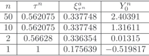
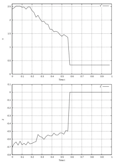
The previous remark entails in particular that (H2) and (H2’) lead to quite different maximization problems. The model under Assumption (H2) is the one which is the most studied in the literature and expresses the fact that with positive probability, the problem (2.1) is the same as the classical maximization problem with terminal time T . Naturally, the expectation formulation puts a weight on the scenarii which, indeed, lead to the classical framework. Assumption (H2’) expresses the fact that with probability 1 the final horizon is less than T (see Figure 2 for an example). This makes the problem completely different since in the first case the agent fears that some random event may happen, whereas in the second case she knows that it is going to happen. As a consequence, these two different assumptions should make some changes in the mathematical analysis. This feature will become quite transparent when solving BSDEs related to the maximi zation problem.
For any mP N˚, we denote by PpFqm(resp. PpGqm) the set of F (resp. G)-predictable
processes valued in Rm. If m“ 1 we simply write PpFq for PpFq1, and the same for G.
We recall from [20, Lemma 4.4] the decomposition of any G-predictable process ψ, given by
Here the process ψ0 is F-predictable, and for a given non-negative u, the process ψ1 tpuq
with tě u, is an F-predictable process. Furthermore, for fixed t, the mapping ψ1 tp¨q is
Ftb Bpr0, 8qq-measurable. Moreover, if the process ψ is uniformly bounded, then it is possible to choose ψ0 and ψ1p.q to be bounded.
We introduce the following spaces ‚ S2
F:“
#
Y “ pYtqtPr0,T sP PpFq, with continuous paths, E
« sup tPr0,T s |Yt|2 ff ă `8 + , ‚ S2 G:“ # Y “ pYtqtPr0,T sP PpGq, with càdlàg paths, E « sup tPr0,T s |Yt|2 ff ă `8 + , ‚ S8F :“ #
Y “ pYtqtPr0,T sP PpFq, with continuous paths, }Y }F,8:“ sup tPr0,T s |Yt| ă `8 + , ‚ S8 G :“ #
Y “ pYtqtPr0,T sP PpGq, with càdlàg paths, }Y }G,8 :“ sup tPr0,T s |Yt| ă `8 + , ‚ H2 F:“ # Z“ pZtqtPr0,T sP PpFqd, E «żT 0 }Zs}2ds ff ă `8 + , ‚ H2 G:“ # Z“ pZtqtPr0,T sP PpGqd, E «żT 0 }Zs}2ds ff ă `8 + , ‚ L2G:“ # U “ pUtqtPr0,T sP PpGq, E «żT 0 |Us|2λsds ff ă `8 + . In the following, let Y be in S8
F (resp. S8G ), for the sake of simplicity, we use the notation
}Y }8 :“ }Y }F,8 (resp. }Y }8 :“ }Y }G,8). We conclude this section with a sufficient
condition for the stochastic exponential of a càdlàg martingale to be a true martingale. Given a G-semimartingale P :“ pPtqtPr0,T s, we denote by EpP q :“ pEpP qtqtPr0,T s its
Doléans-Dade stochastic exponential, defined as usual by: EpP qt:“ exp ˆ Pt´ 1 2rP c, Pcs t ˙ ź 0ăsďt p1 ` ∆sPq exp p´∆sPq ,
with ∆sP :“ Ps´ Ps´ and where Pc denotes the continuous part of P . A càdlàg
G-martingale P is said to be in BMOpP, Gq if }P }2 BMOpP,Gq:“ esssup ρPT pGq E“|PT ´ Pρ´|2|Gρ ‰ ă `8.
For simplicity, we will omit the P-dependence in the space BMOpP, Gq and will only specify the underlying probability measure if it is different from P.
Proposition 2.2. [11, VII.76] The jumps of a BMOpGq martingale are bounded. The previous proposition together with the definition of a BMOpGq martingale imply that it is enough for P to be a BMOpGq martingale, that it has bounded jumps and satisfies: esssup ρPT pGq Er |PT ´ Pρ|2 ˇ ˇ Gρs ă `8.
For the class of BMOpGq martingale we have the following property.
Proposition 2.3. [17, Theorem 2] Assume that P is a G martingale such that there exists c, δą 0 such that ∆τP ě ´1 ` δ and |∆τP| ď c, and which satisfies
esssup
ρPT pGq
ErxP yT ´ xP yρ|Gρs ă `8.
We set for BP tF, Gu H2BMO,PpBq :“ # N “ pNtqtPr0,T sP H2pBq, ˆżt 0 NsdWs ˙ tPr0,T s P BMOpB, Pq + , and use the same convention consisting in omitting the P dependence unless we are working with another probability measure.
3
Exponential utility function
We study in this article a "usual" utility function, namely the exponential function, to solve the utility maximization problem (2.1), which is open in the framework of random time horizon. By open we mean that, even though we have seen that the existence of an optimal strategy for general utility function has been given in [7] using a duality approach, we here aim at characterizing both the optimal strategy π˚ and the value function. To
that purpose, we combine the martingale optimality principle and the theory of BSDEs with random time horizon. Note that in the classical utility maximization problem with time horizon T this technique has been successfully applied in [29] in the exponential framework, and in [16] for the three classical utility functions, that is exponential, power and logarithm.
Recall the maximization problem (2.1) sup
πPA
ErU pXTπ^τ´ ξqs,
where A denotes the set of admissible strategies, that is G-predictable processes with some integrability conditions (precise definitions will be given later on), and ξ is a bounded GT^τ-measurable random variable. At this stage we do not need to make
precise these integrability conditions and the exact definition of the wealth process Xπ.
Let us simply note that by definition an element π of A will satisfy that π1pτ ^T,T s“ 0.
This condition together with the characterization of G-predictable processes recalled in (2.5) entails that π“ ˜π1r0,τ ^T s with ˜πa F-predictable process. Hence in our setting the
strategies are essentially F-predictable.
We now turn to a suitable decomposition of ξ when T ă τ or τ ď T .
Lemma 3.1. Let ξ be a GT^τ-measurable random variable. Then, there exist ξb which
is FT-measurable and an F-predictable process ξa such that
ξ“ ξb
1Tăτ` ξτa1τďT. (3.1)
Proof. Let ξ be a GT^τ-measurable random variable, we have
ξ“ ξ1Tăτ` ξ1τďT,
which can be rewritten as
ξ“ ξb1
Tăτ` ˆξa1τďT,
where ξb is an F
T measurable random variable and ˆξa is Gτ-measurable. According to
[30, Theorem 2.5], since the assumption pH1q holds, we get Fτ “ Gτ, where we recall
that the σ-field Fτ is defined by
Fτ“ σpXτ, X is an F-optional processq.
Hence, from the definition of Fτ, we know that there exists an F-optional process denoted
by ξa such that ˆξa “ ξa
τ, P´ a.s. Since F is the (augmented) Brownian filtration, any
F-optional process is an F-predictable process.
Remark 3.2. In [24], the decomposition (3.1) was taken as an assumption. However thanks to Lemma 3.1, we know that as long as F is the augmented Brownian filtration, it always holds true.
In our framework, the martingale optimality principle can be expressed as follows (we provide a proof for the comfort of the reader even though the arguments are the exact counterpart of the deterministic horizon problem).
Proposition 3.3 (Martingale optimality principle for the random horizon problem). Let Rπ:“ pRπ
tqtPr0,T s be a family of stochastic processes indexed by πP A such that
piq Rπ
T^τ “ U pXT^τπ ´ ξq, @π P A,
piiq Rπ
¨^τ is a G-supermartingale for every π in A,
piiiq Dc P R, Rπ
0 “ c, @π P A,
pivq there exists π˚ in A, such that Rπ˚ is a G-martingale.
Then, π˚ is a solution of the maximization problem (2.1).
Proof. Let π in A. Conditions (i)-(iv) immediately imply that ErU pXπ T^τ´ ξqs piq “ ErRπ T^τs piiq ď Rπ 0 piiiq “ Rπ˚ 0 pivq “ ErRπ˚ T^τs piq “ ErU pXπ˚ T^τ´ ξqs,
which concludes the proof.
Note that until now, we have used neither the definition of A (provided that the expec-tation ErU pXπ
T^τqs is finite) nor the definition of U . However, it remains to construct
this family of processespRπq
πPAand this is exactly at this stage that we need to specify
both the utility function U and the set of admissible strategies A. To this end we set: Vpxq :“ sup
πPA
ErU pXTπ^τ´ ξqs, (3.2)
where Xπ
T^τ denotes the value at time T ^ τ of the wealth process associated to the
strategy π1rt^τ ,T ^τ swith initial capital x at time 0, defined below in (3.3). This amounts
to say that the optimization only holds on the time interval rt ^ τ , T ^ τ s. From now on, we consider the exponential utility function defined as
Upxq “ ´ expp´αxq, α ą 0. In that case we parametrize a Rm-valued strategy π :“ pπ
tqtPr0,T s as the amount of
numéraire invested in the risky asset S (component-wise) so that the wealth process Xπ
associated to a strategy π is defined as: Xtπ “ x ` żt 0 πs¨ σsdWs` żt 0 πs¨ bsds, tP r0, T s. (3.3)
Note that under our assumption on σ (that is σσT is invertible and uniformly elliptic), the
introduction of the volatility process does not bring any additional difficulty compared to the case with volatility one. Indeed, as it is well-known, if we set θ :“ σTpσσTq´1b
and p :“ σTπ, the wealth process becomes
Xtπ“ x ` żt 0 ps¨ dWs` żt 0 ps¨ θsds“: Xtp, tP r0, T s, (3.4)
and a portfolio is described by the process p, which is now Rd-valued. Let C :“ pC tqtPr0,T s
be a predictable process with values in the closed subsets of Rd. As in [15] we define the
set of admissible strategies by
A :“!pP rA, pP H2BMOpGq ) , with r A :“!pptqtPr0,T sP PpGqd, ptP Ct, dtb P ´ a.e., p1pτ ^T,T s“ 0 ) .
Since the liability ξ is bounded, according to [15, Remark 2.1], optimal strategies corre-sponding to the utility maximization problem (2.1) coincide with those of [16]. In order to give a characterization of both the optimal strategy p˚and of the value function Vpxq
defined by (3.2), we combine the martingale optimality principle of Proposition 3.3 and the theory of BSDEs with random time horizon.
Theorem 3.4. Assume that pH1q and pH2q or pH21q hold. Assume that the BSDE
Yt“ ξ ´ żT^τ t^τ Zs¨ dWs´ żT^τ t^τ UsdHs´ żT^τ t^τ fps, Ys, Zs, Usqds, t P r0, T s, (3.5) with fps, ω, z, uq :“ ´α 2dist 2 ˆ z` 1 αθs, Cspωq ˙ ` z ¨ θs` }θs}2 2α ´ λs eαu´ 1 α , (3.6) where dist denotes the usual Euclidean distance, admits a unique solution pin the sense of Definition 4.1q such that Y and U are uniformly bounded and such that ş0¨Zs¨ dWs`
ş¨ 0pe
αUs´ 1qdM
sis a BMOpGq-martingale. Then, the family of processes
Rpt :“ ´ expp´αpXtp´ Ytqq, t P r0, T ^ τ s, p P A,
satisfiespiq ´ pivq of Proposition 3.3, so that
Vpxq “ ´ expp´αpx ´ Y0qq,
and an optimal strategy p˚P A for the utility maximisation problem (3.2) is given by
p˚t P ΠCtpωq ˆ Zt` θt α ˙ , tP r0, T s, P ´ a.s. (3.7) Proof. Assume that the BSDE (3.5) admits a unique solution (in the sense of Definition 4.1) such that Y and U are uniformly bounded and such that
P :“ ż¨ 0 Zs¨ dWs` ż¨ 0 peαUs´ 1qdM s, is a BMOpGq martingale.
Following the initial computations of [16] (see also [2, 27] for the discontinuous case) we set:
Rtp:“ ´ expp´αpXtp´ Ytqq, t P r0, T ^ τ s, p P A.
Clearly, the family of processes Rp satisfies Properties (i) and (iii). By definition each
process Rpreduces to Rpt “ Lptexp ˆżt 0 vps, ps, Zs, Usqds ˙ , with vps, p, z, uq :“ α 2 2 }p ´ z} 2
´ αp ¨ θ ` λspeαu´ 1 ´ αuq ` α1tsďτ ufps, z, uq,
and Lpt :“ ´ expp´αpx ´ Y0qqE ˆ ´α ż¨ 0 pps´ Zsq ¨ dWs` ż¨ 0 peαUs´ 1qdM s ˙ t , which is a uniformly integrable martingale by Proposition 2.3. As in [16], the latter property together with the boundedness of Y and the notion of admissibility for the strategies p imply that each process Rp is a G-supermartingale and that Rp˚ is a
G-martingale with p˚
t P ΠCtpωq
` Zt`θtα
˘
Remark 3.5. In this paper we have considered exponential utility, however the case of power utility and/or logarithmic utility follows the same line as soon as ξ“ 0.
Of course, the above theorem is a verification type result, which is crucially based on the wellposedness of the BSDE (3.5). We have therefore reduced the analysis of the maximization problem to the study of the BSDE (3.5), which is the purpose of the next section.
4
Analysis of the BSDE
(3.5)
4.1
Some general results on BSDEs with random horizon
As we have seen in the previous section, solving the optimal portfolio problem under exponential preferences (with interest rate 0) reduces to solving a BSDE with a random time horizon. This class of equations has been studied in [9], and one could construct a classical theory for these equations. However, in our setting the filtration G is strongly determined by the terminal time τ , and the structure of predictable processes with respect to G is richer than in the general framework. More precisely, from [20] we know that a G-predictable process can be described using F-predictable processes before and after τ as recalled in (2.5).
Recall that by (3.1), any bounded GT^τ-measurable random variable ξ can be written as
ξ“ ξb1
Tăτ` ξτa1τďT,
with ξb a F
T-measurable bounded random variable, and ξa a bounded F-predictable
process.
Taking advantage of this decomposition, the solution triple to a BSDE with random horizon τ has been determined in [24] as the one of a BSDE in the Brownian filtration F suitably stopped at τ (see (4.7)-(4.9) below for a precise statement). However we would like to stress that this result has been obtained under the assumption that λ is bounded which is a stronger assumption than (H2).
We consider a BSDE with random terminal horizon of the form Yt“ ξ ´ żT^τ t^τ fps, Ys, Zs, Usqds ´ żT^τ t^τ Zs¨ dWs´ żT^τ t^τ UsdHs. (4.1)
From (2.5) (see also (4.28) in [24]), we can write
fpt, .q1tăτ “ fbpt, .q1tăτ, (4.2)
where fb: Ωˆ r0, T s ˆ R ˆ Rdˆ R ÝÑ R is F-progressively measurable.
Definition 4.1. A triplet of processes pY, Z, U q in S2
Gˆ H2Gˆ L2G is a solution of the
BSDE (4.1) if relation (4.1) is satisfied for every t in r0, T ^ τ s, P-a.s., Yt“ YT^τ, for
tě T ^ τ , Zt“ 0, Ut“ 0 for t ą T ^ τ on the set tτ ă T u, and
E » –żT^τ 0 |f pt, Yt, Zt, Utq|dt ` ˜żT^τ 0 }Zt}2dt ¸1{2fi fl ă `8. (4.3) Remark 4.2. If f is Lipschitz continuous then the fact that pY, Z, U q are in the space S2Gˆ H2
Gˆ L2G implies that (4.3) holds. However under pH2q or pH2’q, f in (3.6) is not
Lipschitz continuous and the fact thatpY, Z, U q are in the space S2
Gˆ H2Gˆ L2G does not guarantee that E «żT^τ 0 |f pt, Yt, Zt, Utq|dt ff ă `8.
Remark 4.3. Note that the term şt0UsdHs is well-defined since it reduces to Uτ1těτ.
Another formulation of a solution would consist in re-writing (4.1) as: Yt“ ξ ´ żT^τ t^τ rf ps, Ys, Zs, Usq ` λsUssds ´ żT^τ t^τ Zs¨ dWs´ żT^τ t^τ UsdMs, tP r0, T s.
In this case, the integrability condition on the driver basically amounts to ask E «żT 0 λs|Us|ds ff ă `8, which insures that the process U is locally square integrable4
, justifying the definition of the stochastic integralş¨0UsdMs.
Similarly given ξ an FT-measurable map, and f : Ωˆ r0, T s ˆ R ˆ Rd ÝÑ R an
F-progressively measurable mapping, we say that a pair of F-adapted processes pY, Zq where Z is predictable is a solution of the Brownian BSDE:
Yt“ ξ ´ żT t fps, Ys, Zsqds ´ żT t Zs¨ dWs, tP r0, T s, (4.4)
if Relation (4.4) is satisfied and if
E » –żT 0 |f pt, Yt, Ztq|dt ` ˜żT 0 }Zt}2dt ¸1{2fi fl ă `8. (4.5)
We recall the following proposition which has been proved in [24]. Proposition 4.4. AssumepH1q-pH2q. If the pBrownianq BSDE
Ytb“ ξb´ żT t fbps, Ysb, Zsb, ξas´ Ysbqds ´ żT t Zsb¨ dWs, tP r0, T s, (4.6) admits a solution pYb, Zbq in S8
F ˆ H2F, then pY, Z, U q defined as
Yt“ Ytb1tăτ` ξaτ1těτ, (4.7)
Zt“ Ztb1tďτ, (4.8)
Ut“ pξta´ Ytbq1tďτ, (4.9)
is a solution of the BSDE (4.1) in S8
G ˆ H2Gˆ L2G.
The previous proposition is in fact a slight generalization of the original result in [24], since in this reference the authors assume λ to be bounded, which implies condition (H2). In addition, the authors in this reference work with classical solutions in S8
G ˆ H2Gˆ L2G.
However, the proof follows the same lines as the original proof in [24], we just notice that [24, Step 1 and Step 2 of the proof of Theorem 4.3] are unchanged and Step 3 holds under Assumption (H2) noticing that
}U }2 L2
G ď CErΛT^τs ă `8,
since Yb and ξa are in S8 F.
Proposition 4.5. We assumepH1q and pH21q. Let A be a real-valued, F
T-measurable
random variable such that Er|A|2s ă `8. Assume that the BSDE
Yb t “ A ´ żT t fbps, Yb s, Zsb, ξas´ Ysbqds ´ żT t Zb s¨ dWs, tP r0, T s, (4.10) 4
Consider ρn:“ inftt ě ρn´1, |Ut| ě nu and τ0 :“ 0, and remark thatş ρn 0 |Us| 2 λsds“ş ρn´ 0 |Us| 2 λsdsď nşT0 |Us|λsdsă 8, P´a.s.
admits a solution pYb, Zbq in S2
Fˆ H2F. ThenpY, Z, U q given by
Yt “ Ytb1tăτ` ξτa1těτ, (4.11)
Zt “ Ztb1tďτ, (4.12)
Ut “ pξat ´ Ytbq1tďτ, (4.13)
is a solution of (4.1) andpY, Z, U q belongs to S2
Gˆ H2Gˆ S2G.
Proof. We reproduce the proof of [24, Theorem 4.3]. Step 1 and Step 2 are unchanged and prove that for all t P r0, T s, pY, Z, U q defined by (4.11), (4.12) and (4.13) satisfied BSDE (4.1). From the definition of Y , since Yband ξaare in S2
F we deduce that Y P S2G.
from the definition of Z, we deduce that ZP H2 G.
Remark 4.6. Note that in the previous result, the fact that Yb is for example bounded
would not imply that U is in L2
G as λ is not integrable.
Remark 4.7. The previous result is very misleading since the terminal condition A in (4.10) plays no role. More precisely, assume that for two different random variables A1 and A2 such that the associated solutions pYA1, ZA1, UA1q and pYA2, ZA2, UA2q are
bounded and verify that ż¨ 0 ZsAi¨ dWs` ż¨ 0 peαUsAi´ 1qdM s is a BMOpGq-martingale pi “ 1, 2q. Then obviously YA1 ı YA2
, and in light of the proof of Theorem 3.4, the maximization problem (3.2) would then be ill-posed as it would have two different value functions. Even though the notion of strategy we use slightly differs from the one used in [7], this conclusion seems to contradict the well-posedness result obtained in this reference. This remark suggests that it might be possible to solve the Brownian BSDE (4.10) for only one element A. For instance, in the exponential u tility setting, Relation (4.5) suggests that A” ξa
T to solve BSDE (4.10). To illustrate this, we assume that α “ 1 and that
there is no Brownian part. We consider the following Cauchy-Lipschitz/Picard-Lindelöf problem:
y1t“ λtpeξ a
t´yt´ 1q, y T “ A.
Assume that ξa is deterministic, bounded and continuously differentiable. Set x
t:“ eyt.
Hence, the previous ODE can be rewritten: x1t“ λtpeξ
a
t ´ x
tq, xT “ eA.
Thus, we can compute explicitly the uniquepglobalq solution, which is xt“ e´ΛtC` e´Λt
żt 0
eξasλ
seΛsds, tP r0, T s,
where C is in R. Using an integration by part, one gets xt“ e´ΛtC` eξ a t ´ żt 0 pξa sq1eξ a se´ şt sλududs, tP r0, T s.
Letting t go to T , we obtain that we must have xT “ eξ a
T. Therefore there is a solution
if and only if A“ ξa T.
4.2
BSDEs for the utility maximization problem
In this section we focus our attention on a class of BSDEs with quadratic growth, which contains in particular the one used for solving the exponential utility maximization prob-lem. We assume that the generator f of BSDE (4.1) admits for all pt, ω, y, z, uq in r0, T s ˆ Ω ˆ R ˆ Rdˆ R the following decomposition
fpt, ω, y, z, uq “ gpt, ω, y, zq ` λtpωq
1´ eαu
α , (4.14)
Assumption 4.8. piq For every py, zq P R ˆ Rd, gp¨, y, zq is G-progressively
measur-able.
piiq There exists M ą 0 such that for every t P r0, T s, |gpt, 0, 0q| ď M , and for every pt, ω, y, y1, z, z1q P r0, T s ˆ Ω ˆ R ˆ R ˆ Rdˆ Rd,
|gpt, ω, y, zq ´ gpt, ω, y1, zq| ď M |y ´ y1|, and
|gpt, ω, y, zq ´ gpt, ω, y, z1q| ď M p1 ` }z} ` }z1}q}z ´ z1}.
Before going further, notice that under Assumption 4.8, we have the following useful linearization for all tP r0, T s
gpt, ω, y, zq ´ gpt, ω, y1, z1q “ mpt, ω, y, y1qpy ´ y1q ` ηpt, ω, z, z1q ¨ pz ´ z1q, P ´ a.s., (4.15)
where m : r0, T s ˆ Ω ˆ R ˆ R ÝÑ R is G-progressively measurable and such that |mpt, y, y1q| ď M and η : r0, T s ˆ Ω ˆ Rdˆ Rd ÝÑ Rd is G-progressively measurable
and such that
}ηpt, z, z1q} ď M p1 ` }z} ` }z1}q, P ´ a.s.
For simplicity, we will write ηpt, zq instead of ηpt, z, 0q and mpt, yq instead of mpt, y, 0q. Notice that under Assumption 4.8, there exists µą 0 such that for every t P r0, T s and y, zP R ˆ Rd
|gpt, y, zq| ď µp1 ` |y| ` }z}2q, P ´ a.s.
4.2.1
A uniqueness result
We start with a uniqueness result for BSDE (4.1) under the Assumption 4.8.
Lemma 4.9. Assume that pH1q and Assumption 4.8 hold. Under pH2q or pH21q, the
BSDE (4.1): Yt“ ξ ´ żT^τ t^τ Zs¨ dWs´ żT^τ t^τ UsdHs´ żT^τ t^τ fps, Ys, Zs, Usqds, t P r0, T s
admits at most one solutionpY, Z, U q such that Y P S8 G and ż¨ 0 Zs¨ dWs` ż¨ 0 peαUs´ 1qdM sis a BMOpGq martingale.
Remark 4.10. From the orthogonality of W and M , notice that ż¨
0
Zs¨ dWs`
ż¨ 0
peαUs´ 1qdMsis a BMOpGq martingale
ðñ ż¨ 0 Zs¨ dWs and ż¨ 0
peαUs´ 1qdMs are two BMOpGq martingales.
Proof of Lemma 4.9. LetpY, Z, Uq and p rY, rZ, rUq be two solutions of BSDE (4.1) above withpY, rYq P S8
G ˆ S8G and such that
ż¨ 0 Zs¨ dWs` ż¨ 0 peαUs´ 1qdM s and ż¨ 0 r Zs¨ dWs` ż¨ 0 peα rUs´ 1qdM s,
are two BMOpGq martingales. Then pδY :“ Y ´ rY, δZ :“ Z ´ rZ, δU :“ U ´ rUq solves the BSDE: δYt“ 0 ´ żT^τ t^τ δZs¨ dWs´ żT^τ t^τ δUsdHs´ żT^τ t^τ δfpsqds, t P r0, T s,
where
δfpsq :“ gps, Ys, Zsq ´ gps, rYs, rZsq ´ λs
eαUs´ eα rUs
α .
The equation linearizes to obtain δYt“ 0 ´ żT^τ t^τ δYsmps, Ys, pYsq ` δZs¨ ηps, Zs, pZsq ´ λseα pUsδUsds ´ żT^τ t^τ δZs¨ dWs´ żT^τ t^τ δUsdHs, tP r0, T s,
where pUs is a point between Usand rUs, m and η are given by Relation (4.15). Knowing
thatş¨0Zs¨ dWs andş¨0Zrs¨ dWsare two BMOpGq-martingales, from Assumption 4.8piiq
we deduce thatş0¨ηps, Zs, ˜Zsq ¨ dWs is a BMOpGq-martingale and the previous relation
re-writes again as: δYt“ 0 ´ żT^τ t^τ δZs¨ dWsQ´ żT^τ t^τ δUsdMsQ´ żT^τ t^τ δYsmsds, tP r0, T s, (4.16) with dQ dP :“ E ˆ ´ ż¨ 0 ηps, Zs, pZsq ¨ dWs` ż¨ 0 peα pUs´ 1qdM s ˙ T , and WQ:“ W `ş¨ 0ηps, Zs, pZsq ¨ dWsand M Q:“ M ´ş¨ 0pe α pUs´ 1qλ sds. Note that Q is
a well-defined probability measure, as soon as EpP q with P :“ ´ ż¨ 0 ηps, Zs, pZsq ¨ dWs` ż¨ 0 peα xUs´ 1qdM s,
is a true martingale. In that case, the conclusion of the lemma follows by linearization and taking the Q-conditional expectation in (4.16) knowing that m is bounded. It then remains to prove that the process P is a BMOpGq martingale which will imply that its stochastic exponential is a uniformly integrable martingale by Proposition 2.3. Note that sinceş0¨peαUs´ 1qdM
sandş0¨peα rUs´ 1qdMsare two BMOpGq martingales, then according
to Proposition 2.2, Uτ and rUτ are bounded, hence pUτ is bounded by cą 0. We deduce
that the jump of P at time τ is bounded and greater than´1 ` δ with δ :“ e´αc ą 0.
Since pUs is an element between Us and rUs, it is a (random) convex combination of Us
and rUs. The convexity of the mapping xÞÑ |eαx´ 1|2 implies for any element ρ in TpGq
that żT ρ |eα pUs´ 1|2λ sdsď C ˜żT ρ |eαUs´ 1|2λsds` żT ρ |eα rUs´ 1|2λ sds ¸ .
This estimate together with the BMO properties proved so far, imply that P is a BMOpGq martingale.
4.2.2
Existence results for Brownian BSDEs
We turn to the existence of a solution pY, Zq to the BSDE (4.1) such that Y is in S8 G
and ş¨0Zs¨ dWs`ş0¨peαUs ´ 1qdMs is a BMOpGq martingale under Assumptions pH2q
andpH2’q. From Proposition 4.4 and Proposition 4.5, this BSDE can be reduced to the following Brownian BSDE
Ytb “ ξb´żT t gbps, Yb s, Zsbq ` λs 1´ eαpξa s´Ysbq α ds´ żT t Zsb¨ dWs, (4.17)
where gb satisfies Assumption 4.8 (changing in piq G-progressively measurable by
F-progressively measurable) and inherits the decomposition (4.15) from the one of g as gbpt, ω, y, zq ´ gbpt, ω, y1, z1q “ mbpt, ω, y, y1qpy ´ y1q ` ηbpt, ω, z, z1qpz ´ z1q, (4.18)
for any pt, y, y1, z, z1q P r0, T s ˆ R2ˆ pRdq2 with mbpt, ¨q :“ mpt, ¨q1
tďτ and ηbpt, ¨q :“
ηpt, ¨q1tďτ. However, neither AssumptionpH2q nor Assumption pH2’q guarantee directly
that this quadratic BSDE admits a solution. Hence, we use approximation arguments and introduce quadratic BSDEs defined for ně 1 by
Ytb,n “ ξb´ żT t gbps, Yb,n s , Zsb,nq`λns 1´ eαpξas´Yb,n s q α ds´ żT t Zsb,n¨dWs, tP r0, T s, (4.19)
where λn:“ λ ^ n. By developing the integrand in this BSDE (4.19), one obtains
Ytb,n “ ξb´ żT t gbps, Ysb,n, Zsb,nq ´ ˜λb,ns ξsa` ˜λnsYsb,nds´ żT t Zsb,n¨ dWs, tP r0, T s, (4.20) where ˜λn s :“ λns ş1 0e ´αθpYb,n s ´ξsaqdθ.
Lemma 4.11 (General a priori estimates under (H2)). Let ně 0. Under Assumptions pH1q-pH2q and Assumption 4.8, the BSDE (4.19) admits a unique solution pYb,n, Zb,nq P
S8F ˆ H2
BMOpFq such that for all tP r0, T s,
|Ytb,n| ď eM T `}ξb}
8` M pT ´ tq ` }ξa}8˘“: CY,
and}Zb,n} H2
BMOpFq is uniformly bounded in n.
Proof. Let tP r0, T s. The proof is divided in several steps.
Step 1: Uniqueness. Assume that there exist two solutionspYn, Znq P S8
F ˆH2Fand
p ĂYn, ĂZnq P S8
F ˆ H2F to BSDE (4.19) such that }Zn}H2
BMOpFq` } ĂZn}H2
BMOpFq is uniformly
bounded in n. Set δYn :“ Yn´ ĂYn and δZn:“ Zn´ ĂZn, and
| λn s :“ λnseαpξ a s´ĄYsnq ż1 0 e´αθpYsn´ĄYsnqdθ.
ThuspδYn, δZnq is solution of
δYtn“ 0 ´ żT t ηbps, Zsn, rZsnq ¨ δZsn` ´ | λn s` mbps, Ysn, rYsnq ¯ δYsnds´ żT t δZsn¨ dWs. (4.21)
Hence, knowing thatş¨0Zn
s¨ dWsandş¨0Z˜sn¨ dWsare two BMOpFq martingales and using
Assumption 4.8, we know that ηb is in H2
BMOpFqand we can define a probability Q by
dQ dP :“ E ˜ ´ żT 0 ηbps, Zn s, rZsnq ¨ dWs ¸ . Moreover, WQ:“ W `ş¨ 0η bps, Zn
s, rZsnqds is then a Brownian motion under Q. So BSDE
(4.21) rewrites as δYtn“ 0 ´ żT t ´ | λn s ` mbps, Ysn, rYsnq ¯ δYsnds´ żT t δZsn¨ dWQ s . (4.22) Set Ă δYnt :“ e´şt 0λ|ns`mbps,Yns, rYsnqdsδYn t, for all tP r0, T s.
Thenp ĂδYn, ĂδZnq satisfies Ă δYnt “ 0 ´ żT t e´şs0λ|nu`m bpu,Yn u, rY n uqdsδZn s ¨ dW Q s, tP r0, T s,
Step 2: Existence. We turn now to the existence of a solution of BSDE (4.19) in S8F ˆ H2
BMOpFq. Consider the following truncated BSDE
p Ytn“ ξb´ żT t gbps, pYsn, pZsnq ` λns 1´ eαpξa s´ pY n s_p´CYqq α ds´ żT t p Zsn¨ dWs. (4.23)
Then, the classical quadratic BSDE (4.23) admits a unique solution p pYn, pZnq P S8 F ˆ
H2BMOpFq(see e.g. [25]). We can then rewrite BSDE (4.23) as
p Ytn“ ξb´ żT t ´ gbps, 0, 0q `´λ˜ns1Ypn sě´CY ` m bps, pYn s q ¯ p Ysn´ ˜λnsξsa1Ypn sě´CY ` λn s 1´ eαpξa s`CYq α 1Ypn să´CY ` η bps, pZn sq ¨ pZsn ¯ ds´ żT t p Zsn¨ dWs, (4.24) where ˜λn s :“ λs^ n ş1 0e´αθp p Yn s´ξsaqdθ. Set γnpsq :“ ˜λn s1| pYn s|ďCY ` m bps, pYn s q and Yn:“ pYne´ ş¨ 0γ npsqds
, we obtain from BSDE (4.24) Ytn“ ξbe´şT0γ n udu´ żT t e´şs0γ n udu ´ gbps, 0, 0q ´ ˜λnsξsa1Ypn sě´CY ¯ ds ´ żT t e´şs0γ n uduλn s 1´ eαpξa s`CYq α 1Ypn să´CYds´ żT t e´şs0γ n uduZpn s ¨ dWQ n s , tP r0, T s, where dQn “ Ep´şT 0 η bps, pZn sq ¨ dWsqdP and WQ n :“ W `ş0¨ηbps, pZn sqds is a Brownian
motion under the probability Qn, sinceş¨ 0η
bps, pZn
sq ¨ dWs is a BMOpFq-martingale from
Assumption 4.8piiq. Increasing the constants if necessary, we have ξa ě ´C
Y, then
taking the conditional expectation under Qn we deduce that
p Ytn ě ´eM T´}ξb}8` M pT ´ tq ` }ξa}8EQ n” żT t e´ şs t˜λ n u1xY nu ě´CYduλ˜n s1Ypn sě´CYds looooooooooooooooooooooomooooooooooooooooooooooon :“I ˇ ˇ ˇFt ı¯ . Since I “ 1´e´ şT t λ˜ n
u1xY nu ě´CYduď 1, we deduce that pYn
t ě ´CY. A posteriori, we deduce
that the solution p pYn, pZnq of BSDE (4.23) is in fact the unique solution pYb,n, Zb,nq of
BSDE (4.19) in S8
F ˆ H2BMOpFq such that Y b,n
t ě ´CY, tP r0, T s, P ´ a.s. Then, using a
linearization and taking the conditional expectation under Qn, we can compute explicitly
Yb,n from BSDE (4.20) Ytb,n“ ´EQn « ξbe´şTt γ n udu` żT t e´şstγ n udu ´ gbps, 0, 0q ´ ˜λnsξa¯ds ˇ ˇ ˇ ˇ ˇFt ff ď eM Tp}ξb} 8` M pT ´ tq ` }ξa}8q.
Step 3: BMO norm of Zb,n. Let ρP T pFq be a random horizon and β a positive
constant. Using Itô’s formula, we obtain eβYρb,n “ eβξ b ´ żT ρ βeβYsb,n ˜ gbps, Yb,n s , Zsb,nq ` λns 1´ eαpξa s´Y b,n s q α ¸ ds ´ żT ρ βeβYsb,nZb,n s ¨ dWs´ β2 2 żT ρ eβYsb,n}Zb,n s }2ds.
Hence, from AssumptionpH1q, using the fact that, by Step 2, Yb,nis uniformly bounded
in n by CY and taking conditional expectations, we deduce
β2 2 E « żT ρ eβYsb,n}Zn s}2ds ˇ ˇ ˇ ˇ ˇFρ ff ď eβ}ξb}8 ` βE « żT ρ eβYsb,n|gbps, Yb,n s , Zsb,nq|ds ˇ ˇ ˇ ˇ ˇFρ ff ` βeβCY 1` e αp}ξa}8`CYq α E « żT ρ λsds ˇ ˇ ˇ ˇ ˇFρ ff .
Since|gbps, y, zq| ď µp1 ` |y| ` }z}2q we obtain
ˆ β2 2 ´ µβ ˙ E « żT ρ eβYsn}Zb,n s }2ds ˇ ˇ ˇ ˇ ˇFρ ff ď eβ}ξb}8` βeβCYT µp1 ` CYq ` βeβCY1` eαp}ξ a}8`CYq α E « żT ρ λsds ˇ ˇ ˇ ˇ ˇFρ ff .
By choosing β ą 2µ, under Assumption (H2) and using the boundedness of Yb,n, we
deduce that E « żT ρ › ›Zb,n s › ›2 ds ˇ ˇ ˇ ˇ ˇFρ ff ď Cβ, where Cβ :“ e2βCY « 1` β ˜ 1` eαp}ξa}8`CYq α E « żT ρ λsds ˇ ˇ ˇ ˇ ˇFρ ff ` T µp1 ` CYq ¸ff ˆ β2 1 2 ´ µβ .
Then, under AssumptionpH2q, }Zb,n} H2
BMOpFqis uniformly bounded in n.
Theorem 4.12. Let AssumptionspH1q-pH2q and Assumption 4.8 hold. Then the Brow-nian BSDE Ytb“ ξb´ż T t gbps, Yb s, Zsbq ` λs 1´ eαpξa s´Y b sq α ds´ żT t Zsb¨ dWs, tP r0, T s, (4.25)
admits a unique solution pin S2
Fˆ H2Fq. In addition, Yb is bounded and
ş¨ 0Z
b
s¨ dWs is a
BMOpFq-martingale.
Proof. The proof is based on an approximation procedure using BSDE (4.20). The aim of this proof is to show that the solutionpYn, Znq to this approached BSDE converges
in S8
F ˆ H2BMOpFqto the solution of BSDE (4.25). Let p, qě n, we denote δYt:“ Ytp´ Y q t
and δZt:“ Ztp´ Z q
t for all tP r0, T s. Then, pδY, δZq is solution of the following BSDE
δYt“ ´ żT t mbps, Yp s, YsqqδYs` ηbps, Zsp, Zsqq ¨ δZs` λps 1´ eαpξa s´Y p sq α ds ´ żT t λqs1´ e αpξa s´Ysqq α ds´ żT t δZs¨ dWs,
which can be rewritten as δYt“ ´ żT t λps´ λq s α ` pλ p s´ λqsq eαpξas´Y p sq α looooooooooooooooooomooooooooooooooooooon :“ϕp,qs `´λqseαpξas´Ysq` mbps, Yp s, Ysqq ¯ δYsds ´ żT t δZs¨ dWQ n s ,
where Y is a process lying between Yp and Yq which satisfies for all sP rt, T s, |Y s| ď
CY, P´ a.s., and where WQ n
:“ W `ş¨0ηbps, Zp
s, Zsqqds is a Brownian motion under Qn
given by dQn dP “ E ˜ ´ żT 0 ηbpt, Ztp, Ztqq ¨ dWt ¸ , which is well defined sinceş¨0ηbps, Zp
s, Zsqq¨dWsis a BMOpFq martingale from Assumption
4.8. Let βě 0, using Itô’s formula eβt|δYt|2“ 0 ´ żT t 2eβsδYsϕp,qs ` eβs ´ 2λqseαpξas´Ysq` 2mbps, Ysp, Ysqq ` β ¯ |δYs|2ds ´ 2 żT t eβsδYsδZs¨ dWQ n s ´ żT t eβs}δZs}2ds.
Using the non-negativity of λq and choosing βą 2M , we deduce that
eβt|δYt|2ď 0 ´ żT t 2eβsδYsϕp,qs ds´ 2 żT t eβsδYsδZs¨ dWQ n s ´ żT t eβs}δZs}2ds.
Then, using the boundedness of Yn uniformly in n, there exists a positive constant C
such that EQn « sup tPr0,T s |δYt|2 ff ` EQn«żT 0 }δZs}2ds ff ď CEQn«żT 0 |λp s´ λqs|ds ff , Hence, EQn « sup tPr0,T s |δYt|2 ff ď CEQn«żT 0 |λp s´ λqs|ds ff . (4.26)
We want to obtain this kind of estimates under the probability P. Notice that
E « sup tPr0,T s |δYt|2 ff “ EQn » –E ˜ ´ żT 0 ηbpt, Ztp, Ztqq ¨ dWt ¸´1 sup tPr0,T s |δYt|2 fi fl “ EQn « E ˜żT 0 ηbpt, Ztp, Ztqq ¨ dWtQn ¸ sup tPr0,T s |δYt|2 ff .
From Assumption 4.8 and Lemma 4.11, ş0¨ ηbps, Zn
sq ¨ dWs is a BMO(F) martingale and
}ηbp¨, Zn
¨ q}H2BMOpFq is uniformly bounded in n. Then according to [23, Theorem 3.3],
ş¨
0ηbps, Zsnq ¨ dWQ n
s is a BMO(Qn, F) martingale. Moreover, following the proof of [23,
Theorem 3.3] together with the proof of [23, Theorem 2.4], it is easily verified that }ηbp¨, Zn
¨ q}H2
BMOpQn,Fq is uniformly bounded in n. Thus, from [23, Theorem 3.1] there
exists rą 1 (its conjugate being denoted by r) such that sup ně1 EQn « E ˜żT 0 ηbpt, Ztp, Z q tq ¨ dW Qn t ¸rff ă `8.
Since Yn is uniformly bounded in n, we deduce that there exists ką 0 such that
E « sup tPr0,T s |δYt|2 ff ď EQn « E ˜żT 0 ηbpt, Ztp, Z q tq ¨ dW Qn t ¸rff1r EQn « sup tPr0,T s |δYt|2r ff1 r ď kEQn « sup tPr0,T s |δYt|2 ff1 r . (4.27)
Similarly, from the definition of Qn there exists Ką 0 such that EQn «żT 0 |λp s´ λqs|ds ff ď KE » –˜żT 0 |λp s´ λqs|ds ¸rfi fl 1 r . (4.28)
Thus, from Inequalities (4.26), (4.27) and (4.28), we deduce that there exists a positive constant κ such that Inequality (4.26) rewrites
E « sup tPr0,T s |δYt|2 ff ď κE » –˜żT 0 |λps´ λqs|ds ¸rfi fl 2 r ÝÑ nÑ80,
by dominated convergence and using (2.3).
Then, we deduce that Yn is a Cauchy sequence in S2
F. Hence, Yn converges in S2F to a
process Y . Besides, since Yb,nis uniformly bounded in n, taking a subsequence (which we
still denotepYb,nq
ně0for simplicity), of uniformly bounded process in n which converges,
P´ a.s., to Yb, we deduce that Yb P S8
F. Thus, by Lebesgue’s dominated convergence
Theorem, Yb,n converges to Yb in Sp
F for every pě 1. Recall that
Ytb,n“ ξb´żT t gbps, Yb,n s , Zsb,nq ` ˜λnsYsb,n´ ˜λnsξasds´ żT t Zsb,n¨ dWs, where ˜λn s :“ λns ş1 0e ´αθpYb,n
s ´ξsaqdθ, which can be rewritten
Ytb,n“ Y0b,n` żt 0 Ab,ns ds` żt 0 Zsb,n¨ dWs, where An
s :“ gbps, Ysb,n, Zsb,nq ` ˜λnsYsb,n´ ˜λnsξas. Knowing that limnÑ8}Yb,n´ Yb}SpF “ 0
for every pě 1, we deduce from Theorem 1 in [1] that Yb is a semimartingale such that
Yb t “ Y0b` şt 0Asds` şt 0Z b
s¨ dWs, where for all pě 1
E «˜ sup tPr0,T s żt 0 Zsb¨ dWs ¸pff ď K, E «˜żT 0 |As|ds ¸pff ď K, for some positive constant K, and
lim nÑ8E » –˜żT 0 |Zsb,n´ Zsb|2ds ¸p 2fi fl “ 0, lim nÑ8E «˜żT 0 |Ans ´ As|ds ¸pff “ 0. Since ş¨0Zb,n
s ¨ dWs is a BMO(F) martingale, there exists K1 ą 0 such that }Zb,n}HpF `
}Zb} HpF ď K
C which may vary from line to line such that E «ˆżt 0 |An s´ ´ gbps, Yb s, Zsbq ` ˜λsYsb´ ˜λsξsa ¯ |ds ˙pff ď C ˜ E «ˆżt 0 |Yb s ´ Ysb,n|ds ˙pff ` E «ˆżt 0 p1 ` }Zb s} ` }Zsb,n}q}Zsb´ Zsb,n}ds ˙pff ` E «ˆżt 0 ˇ ˇ ˇ˜λsYsb´ ˜λnsYsb,n ˇ ˇ ˇ ds ˙pff ` E «ˆżt 0 ˇ ˇ ˇ˜λs´ ˜λns ˇ ˇ ˇ |ξsa|ds ˙pff ¸ ď C ˜ }Yb´ Yb,n}Sp` E «˜żT 0 }Zsb,n´ Zsb}2ds ¸pff12 ` E «ˆżt 0 |λs´ λns|ds ˙pff ` }Yb,n´ Yb}SpFErΛ p ts ¸ ÝÑ nÑ80.
Then, we deduce that there exists a F-predictable process Zb such that
Ytb“ Y0b` żt 0 gbps, Ysb, Zsbq ` ˜λsYsb´ ˜λsξasds` żt 0 Zsb¨ dWs.
Following the Step 3 in the proof of Lemma 4.11, we deduce that Zb P H2
BMOpFq Then,
the pairpYb, Zbq P S8ˆ H2
BMOpFqbuilt previously is the unique solution of BSDE (4.25),
the uniqueness coming from Lemma 4.9 together with Proposition 4.4.
We now turn to Assumption pH2’q. Notice that the proof of Theorem 4.12 fails under pH2’q since E rΛTs “ 8. We need more regularity on ξa to get a sign on Yb,n, the first
component of the solution of the approached BSDE (4.19) in order to prove that BSDE (4.17) admits a solution under pH2’q.
Assumption 4.13. ξa is a bounded semi-martingale such that
ξat “ ξ0a` żt 0 Dsds` żt 0 γs¨ dWs,
where D, γ are bounded processes satisfying for all sP r0, T s, gbps, ξa
s, γsq ´ Dsě 0.
Before going further, to solve the utility maximization problem (2.1) according to The-orem 3.4, we have to prove thatş¨0ZsdWs`ş0¨peαUs ´ 1qdMs is a BMOpGq-martingale.
Under AssumptionpH2q, this property comes for free from the BMOpFq-martingale prop-erty ofş0¨Zb
sdWs and the boundedness of Yb. However, underpH2’q it is not clear that
whether the BMOpFq-martingale property implies the BMOpGq-martingale property. It is why we show that underpH2’q, BSDE (4.17) admits a unique solution in S8
FˆH2BMOpGq,
as a consequence of the Immersion hypothesis, which is itself a consequence ofpH1q. Lemma 4.14. Assume thatpH1q-pH2’q and Assumptions 4.8 and 4.13 hold. Then, the following BSDE Ytb “ A ´ żT t gbps, Yb s ` ξas, Zsb` γsq ´ Ds` λsfpYsbqds ´ żT t Zsb¨ dWs, (4.29)
where fpxq :“ 1´eα´αx admits a solution in S8
F ˆ H2BMOpGq if and only of A” 0. In this
case, the solution is unique.
Proof. Assume that A ” 0. We aim at showing that BSDE (4.29) admits a (unique) solution in S8
F ˆ H2BMOpGq. Consider the truncated BSDE
Ytb,n“ 0 ´ żT t gbps, Ysb,n` ξsa, Zsb,n` γsq ´ Ds` λnsfpYsb,nqds ´ żT t Zsb,n¨ dWs, (4.30)
which can be rewritten under Assumption 4.8 Ytb,n“ 0 ´ żT t gbps, ξa s, γsq ´ Ds` msYsb,n` ηs¨ Zsb,n` ˜λnsYsb,nds´ żT t Zsb,n¨ dWs, with ms:“ mps, Ysb,n`ξsa, ξsaq, ηs:“ ηps, Zsb,n`γs, γsq and ˜λns :“ λns ş1 0e´αθY b,n s dθ. Then,
following Step 1 and Step 2 in the proof of Lemma 4.11 and since gbps, ξa
s, γsq´Dsis
non-negative under Assumption 4.13, we show that BSDE (4.30) admits a unique solution pYb,n, Zb,nq P S8
F ˆ H2BMOpFq such that
´ eM TpT ´ tq ˜M ď Yb,n
t ď 0, for all t P r0, T s, P ´ a.s., (4.31)
where ˜M is a positive constant. We show now that the H2
BMOpGq norm of Zb,n does not
depend on n by following Step 3 of the proof of Lemma 4.11. Let ρP T pGq be a random horizon and βă 0. Using Itô’s formula, we obtain
eβYρb,n“ 1 ´ żT ρ βeβYsb,n ˜ gbps, Yb,n s ` ξsa, Zsb,n` γsq ´ Ds` λns 1´ e´αYb,n s α ¸ ds ´ żT ρ βeβYsb,nZb,n s ¨ dWs´ β2 2 żT ρ eβYsb,n}Zb,n s }2ds.
Hence, using the fact that Yb,n is non positive and uniformly bounded in n and taking
conditional expectations, we have for any ρP T pGq, from the Immersion property pH1q |β|2 2 E « żT ρ eβYsb,n}Zb,n s }2ds ˇ ˇ ˇ ˇ ˇGρ ff ď 1 ` |β|E « żT ρ eβYsb,n|D s|ds ˇ ˇ ˇ ˇ ˇGρ ff ` |β|E « żT ρ eβYsb,n|gbps, Yb,n s ` ξsa, Zsb,n` γsq|ds ˇ ˇ ˇ ˇ ˇGρ ff .
Since ξa, D and γ are bounded, using the fact that |gbps, y, zq| ď µp1 ` |y| ` }z}2q, we
obtain ˆ|β|2 2 ´ 2µ|β| ˙ E « żT ρ eβYsb,n}Zb,n s }2ds ˇ ˇ ˇ ˇ ˇGρ ff ď e|β|}ξb}8` |β|eβ}Yb,n}8Cp1 ` }Yb,n}8q,
with C ą 0. Choosing β ą 4µ and using the boundedness of Yb,n uniformly in n, we
deduce that there exists a constant Cą 0 which does not depend on n such that E «żT ρ }Zb,n s }2ds ˇ ˇ ˇ ˇ ˇGρ ff ď C. Thus,}Zb,n} H2
BMOpGq is uniformly bounded in n.
We prove now the convergence of the sequencepYb,nq in Sp
F for every p in order to apply
Theorem 1 of [1]. Recall that Ytb,nď 0, for every t P r0, T s. Then, from the comparison
theorem for quadratic BSDEs (see e.g. [25, Theorem 2.6]) and since Yb,nis non positive,
the sequencepYb,nq
n is non-decreasing. Hence, it converges almost surely to
Ytb:“ lim
nÑ8Y b,n
t such that´eM TpT ´ tqM ď Ytbď 0 for all t P r0, T s.
Fix 0ă t0 ă T , we notice that pYb,n, Zb,nq is also the solution to the following BSDE
for 0ď t ď t0 Ytb,n“ Yt0b,n` żt0 t gbps, Ysb,n` ξsa, Zsb,n` γsq ´ Ds` λnsfpYsb,nqds ´ żt0 t Zsb,n¨ dWs.
Hence, for every ně 1 and p, q ě n, by setting δY :“ Yb,p´ Yb,q and reproducing the
proof of Theorem 4.12 with t0 ă T as terminal time instead of T , we deduce that for
every rě 0 there exists Crą 0 which does not depend on p, q such that
E « sup tPr0,t0s |δYt|2 ff ď Cr ¨ ˝E“|δYt0|2‰` E «ˆżt0 0 |λp s´ λqs|ds ˙rff2r˛ ‚. Hence, there exists ˜Cą 0 such that for every n ě 0
sup p,qěn E « sup tPr0,t0s |δYt|2 ff ď ˜C ¨ ˝E”|Ytb,n0 ´ Y b t0| 2ı` E «ˆżt0 0 |λn s ´ λs|ds ˙rff2r˛ ‚. By Lebesgue’s dominated convergence Theorem and since E“Λr
t0 ‰ ă 8, we deduce that the sequencepYb,n1 r0,t0sq is a Cauchy sequence in S 2
F, and knowing that Ynis uniformly
bounded in n,pYb,n1
r0,t0sq is a Cauchy sequence in S p
Ffor every pě 1. Thus, Yb,n1r0,t0s
converges to Yb1
r0,t0s in S p
F for every pě 1. As in the proof of Theorem 4.12, we deduce
from Theorem 1 in [1] that Yb is a semimartingale such that for every tă T ,
Ytb“ Yb 0 ` żt 0 Asds` żt 0 Zsb¨ dWs,
where for all pě 1 and 0 ď t0ă T
E «˜ sup tPr0,t0s żt 0 Zsb¨ dWs ¸pff ď K, E «ˆżt0 0 |As|ds ˙pff ď K, for some Ką 0, and
lim nÑ8E «ˆżt0 0 |Zb,n s ´ Zsb|2ds ˙p 2ff “ 0, lim nÑ8E «ˆżt0 0 |An s´ As|ds ˙pff “ 0. Hence, there exists a F-predictable process Zb such that for every 0ď t ă T
Ytb“ Y0b` żt 0 gbps, Ysb` ξsa, Zsb` γsq ´ Ds` ˜λsYsbds` żt 0 Zsb¨ dWs.
Thus, for ε ą 0 we deduce that there exists a F-predictable process Zb such that for
every 0ď t ă T Yb t “ YpT ´εq_tb ´ żpT ´εq_t t gbps, Yb s`ξsa, Zsb`γsq´Ds`˜λsYsbds` żpT ´εq_t t Zb s¨dWs. (4.32) Moreover using (4.31) |YpT ´εq_tb | “ lim nÑ8|Y b,n pT ´εq_t| ď εM e µT ÝÑ εÑ00“ Y b T, which implies Yb
t is continuous at t“ T . Then, taking the limit when ε goes to 0 in
(4.32), the pair of processes pYb, Zbq satisfies BSDE (4.29). Besides, we have proved
that Yb is in S8
F and non positive. Hence, following the same lines of the proof of the
uniform boundedness of}Zb,n} H2
BMOpGq, we deduce that}Z b}
H2
BMOpGqă `8. Since Yb is
bounded and since}Zb}
H2BMOpGq ă `8, we deduce that pYb, Zbq is the unique solution
in S8
F ˆ H2BMOpGq of (4.29), in the sense of Definition 4.5.
Assume now that there exists a solution pYb, Zbq. Following the Step 1 of the proof of
Theorem 4.15. Assume pH1q-pH2’q hold. Assume moreover that Assumption 4.13 holds. Then under Assumption 4.8 the BSDE
Yb t “ ξTa ´ żT t fbps, Yb s, Zsb, ξsa´ Ysbqds ´ żT t Zb s¨ dWs, tP r0, T s, (4.33) with fbps, y, z, uq :“ gbps, y, zq ` λs 1´ eαu α , admits a unique solution such that Ybis bounded andş¨
0Z b
sdWsis a BMOpGq-martingale.
Proof. Consider the following BSDE ˜ Yb t “ 0 ´ żT t gbps, ˜Yb s ` ξsa, ˜Zsb` γsq ´ Ds` λsf˜p ˜Ysbqds ´ żT t ˜ Zb s¨ dWs, (4.34) where ˜fpxq :“ 1´e´αx
α . Then, according to Lemma 4.14, BSDE (4.34) admits a unique
solution p ˜Yb, ˜Zbq P S8ˆ H2
BMOpGq. By setting Ytb :“ ˜Ytb` ξta and Ztb :“ ˜Ztb` γt, we
deduce thatpYb, Zbq is the unique solution of (4.33) in S8
F ˆ H2BMOpGq.
Remark 4.16. Even if Assumption 4.13 is not too restrictive, especially from the point of view of financial application, we would like to point out the fact that it is not a necessary condition. Consider for simplicity the setting corresponding to α“ 0, and assume that ξa is a deterministic continuous function of timepwhich may be of unbounded variation
and thus not a semimartingaleq, and consider under pH2’q the following linear BSDE Yt“ ξTa ` żT t λspξsa´ Ysqds ´ żT t Zs¨ dWs. (4.35)
Assume that it admits a solution. Then, we necessarily have Yt“ E « żT t λse´ şs tλuduξa sds ˇ ˇ ˇ ˇ ˇFt ff .
Since ξa is automatically uniformly continuous onr0, T s, there is some modulus of
con-tinuity ρ such that
|YT´ε´ ξTa| ď ρpεqE « żT T´ε λse´ şs T´ελududs ˇ ˇ ˇ ˇ ˇFT´ε ff “ ρpεq, so that we obtain YT´εÝÑ ξTa when εÝÑ 0.
However, we cannot hope to solve BSDE (4.35) without assuming at least that ξa is
left-continuous at time T . Indeed, assume that ξa “ 1
r0,T q and choose λs“ T1´s. Then,
YT´ε“ ´1 Û εÑ0ξ
a T “ 0,
which means in this case that BSDE (4.35) does not admit a solution.
The previous remark leads us to hypothesize that Assumption 4.13 is not necessary to obtain existence and uniqueness of the solution to BSDE (4.33). We give the following conjecture that we leave for future research.
Conjecture. AssumepH1q-pH2’q hold and that gbps, 0, 0q is non-negative for every s P
r0, T s. Then under Assumption 4.8 the BSDE Ytb“ ξa T´´ żT t fbps, Yb s, Zsb, ξas´ Ysbqds ´ żT t Zsb¨ dWs, tP r0, T s, with fbps, y, z, uq :“ gbps, y, zq ` λ s 1´ eαu α admits a unique solution such that Ybis bounded andş¨
0Z b
4.3
Existence and uniqueness Theorem for BSDE
(4.1)
Theorem 4.17. Let Assumptions 4.8 and pH1q-pH2q be in force. Then under pH2q prespectively under pH21q and Assumption 4.13q, BSDE (4.1) precalled belowq
Yt“ ξ ´ żT^τ t^τ Zs¨ dWs´ żT^τ t^τ UsdHs´ żT^τ t^τ fps, Ys, Zs, Usqds, t P r0, T s,
admits a unique solutionpY, Z, U q such that Y and U are in S8 G and ş¨ 0Zs¨dWs` ş¨ 0pe αUs´ 1qdMsis a BMOpGq-martingale.
Proof. We have shown the uniqueness of the solution in Lemma 4.9. The existence underpH2q (resp. pH2’q) of a triplet of processes pY, Z, U q satisfying BSDE (4.1), comes directly from Theorem 4.12 (resp. Theorem 4.15) together with Proposition 4.4 (resp. Proposition 4.5). We know moreover that Y and U are in S8
G and using the Immersion
hypothesis, as a consequence ofpH1q, ş¨0Zs¨ dWs is a BMOpGq martingale. Recall that
Us “ pξas ´ Ysbq1sďτ, where Yb is the first component of the solution of the Brownian
BSDE (4.17). We prove thatş¨0peαUs´ 1qdM
s is a BMOpGq martingale
UnderpH2q. We obtain directly from the definition of pH2q and since Yb, ξaare bounded
esssupρPT pGqE « żT ρ |eαpξsa´Ytbq´ 1|2λ tdt ˇ ˇ ˇ ˇ ˇGρ ff ă `8.
Under pH2’q. We first consider the Brownian BSDE (4.34) that we recall ˜ Ytb“ 0 ´ żT t gbps, ˜Ysb` ξa s, ˜Zsb` γsq ´ Ds` λsf˜p ˜Ysbqds ´ żT t ˜ Zsb¨ dWs,
where ˜fpxq :“ 1´eα´αx. Using Decomposition (4.18), we obtain ˜ Ytb“ 0 ´ żT t gbpt, ξa s, γsq ´ Ds` mbpt, ˜Ysb` ξsa, ξsaq ˜Ysb` ηbpt, Zsb` γs, γsq ¨ ˜Zsbds ´ żT t λs 1´ e´α ˜Yb s α ds´ żT t ˜ Zsb¨ dWs,
which can be rewritten ˜ Ytb “ 0 ´ żT t gbpt, ξsa, γsq ´ Ds` pmbpt, ˜Ysb` ξsa, ξsaq ` ˜λsq ˜Ysb` ηbpt, ˜Zsb` γs, γsq ¨ ˜Zsbds ´ żT t ˜ Zsb¨ dWs, tP r0, T s, (4.36) where ˜λs:“ λsş10e´αθ ˜Y b
sdθ. Since mb is bounded by M ą 0, following the proof of [18,
Theorem 4.4] we can easily show5 that
´eM TeΛtE « żT t e´Λspϕs` |ηps, ˜Zsb` γs, γsq ¨ ˜Zsb|qds ˇ ˇ ˇ ˇ ˇGt ff ď ˜Ytbď 0, @t P r0, T s, where ϕs:“ gbpt, ξsa, γsq´Dsis non-negative and Λs“şs0λudu. For the sake of simplicity,
we set ηs:“ ηps, ˜Zsb` γs, γsq and C a positive constant which may vary from line to line.
5
Taking fpxq “ 1´e´αx
α , δ“ 1 in [18, Theorem 4.4] and changing ˜λin [18, Relation (4.4)] by ˜λ ` m b.
Since ˜Yb is bounded and non-positive, it holds that E « żT^τ ρ |e´α ˜Ysb´ 1|2λ sds ˇ ˇ ˇ ˇ ˇGρ ff ď CE « żT^τ ρ |e´α ˜Ysb´ 1|λ sds ˇ ˇ ˇ ˇ ˇGρ ff ď CE « żT^τ ρ p´ ˜Ysbqλsds ˇ ˇ ˇ ˇ ˇGρ ff ď CE « żT^τ ρ E « żT s e´Λupϕu` |ηu¨ ˜Zub|qdu ˇ ˇ ˇ ˇ ˇGs ff eΛsλsds ˇ ˇ ˇ ˇ ˇGρ ff “ CE « żT 0 E « 1τěsěρ żT s e´Λupϕu` |ηu¨ ˜Zub|qdu eΛsλs ˇ ˇ ˇ ˇ ˇGs ff ds ˇ ˇ ˇ ˇ ˇGρ ff “ CE « żT^τ 0 1sěρ żT s e´Λupϕu` |ηu¨ ˜Zub|qdu eΛsλsds ˇ ˇ ˇ ˇ ˇGρ ff ď CpEρ1` E2ρq, where E1ρ:“ E « żT^τ ρ żT s e´Λuϕudu eΛsλsds ˇ ˇ ˇ ˇ ˇGρ ff , and E2ρ:“ E « żT^τ ρ żT s e´Λu|ηu¨ ˜Zub|du eΛsλsds ˇ ˇ ˇ ˇ ˇGρ ff .
On the one hand, knowing that ϕ is bounded and using the integration by part formula, we obtain E1ρď C ˜ E « żT^τ ρ żT s e´Λudu eΛsλsds ˇ ˇ ˇ ˇ ˇGρ ff¸ ď C ˜ E « lim sÑT ^τe Λs żT s e´Λudu´ eΛρ żT ρ e´Λudu ˇ ˇ ˇ ˇ ˇGρ ff ` pT ´ ρq ¸ ď C,
where C ą 0 does not depend on ρ. On the other hand, using the fact that ˜ZbP H2 BMOpGq
and from the existence of a positive constant M1 such that η
u :“ ηps, ˜Zub ` γu, γuq ď M1p1 ` } ˜Zub}q, we get E2ρ“ CE « lim sÑT ^τe ΛsżT s e´Λu|ηu¨ ˜Zub|du ´ eΛρ żT ρ e´Λu|ηu¨ ˜Zub|du ` żT^τ ρ |ηu¨ ˜Zub|du ˇ ˇ ˇ ˇ ˇGρ ff ď C1,
where C1ą 0 does not depend on ρ. We have thus shown that under pH2’q
esssup ρPT pGq E « żT ρ |e´α ˜Ysb´ 1|2λ sds ˇ ˇ ˇ ˇ ˇGρ ff ă `8. (4.37)
By considering p ˜Yb, ˜Zbq the unique solution of BSDE (4.34), previously studied, and denoting bypYb, Zbq the unique solution of BSDE (4.33), we know that Yb“ ˜Yb` ξa
s.
So according to Inequality (4.37), we obtain esssup ρPT pGq E «żT ρ |eαpξsa´Ysbq´ 1|2λ sds ˇ ˇ ˇ ˇ ˇGρ ff ă `8. (4.38)