Theoretical and phenomenological aspects of non-singular black holes

HAL Id: tel-02413360

https://tel.archives-ouvertes.fr/tel-02413360v2

Submitted on 25 Jan 2020

HAL is a multi-disciplinary open access archive for the deposit and dissemination of sci-entific research documents, whether they are pub-lished or not. The documents may come from teaching and research institutions in France or abroad, or from public or private research centers.

L’archive ouverte pluridisciplinaire HAL, est destinée au dépôt et à la diffusion de documents scientifiques de niveau recherche, publiés ou non, émanant des établissements d’enseignement et de recherche français ou étrangers, des laboratoires publics ou privés.

non-singular black holes

Frederic Lamy

To cite this version:

Frederic Lamy. Theoretical and phenomenological aspects of non-singular black holes. Other. Uni-versité Sorbonne Paris Cité, 2018. English. �NNT : 2018USPCC203�. �tel-02413360v2�

T

HÈSE DE

D

OCTORAT

de l’Université Sorbonne Paris Cité

Préparée à l’Université Paris Diderot

École doctorale des Sciences de la Terre et de l’Environnement et Physique de l’Univers, Paris -ED 560

Laboratoire AstroParticule et Cosmologie (APC)

P

HYSIQUE THÉORIQUE

Theoretical and phenomenological aspects of

non-singular black holes

Frédéric Lamy

Thèse dirigée par Pierre Binétruy†et David Langlois,

présentée et soutenue publiquement le 21 septembre 2018 devant un jury composé de :

Dr. Alessandro Fabbri (Enrico Fermi Ctr. (Rome), LPT Orsay) Examinateur

Dr. Eric Gourgoulhon (CNRS, LUTH) Examinateur

Pr. Ruth Gregory (Durham University) Rapporteure

Pr. Carlos Herdeiro (Universidade de Aveiro) Rapporteur

Dr. David Langlois (CNRS, APC) Directeur de thèse

À Pierre.

R

EMERCIEMENTS

La thèse est une aventure à au moins trois égards, en ce qu’elle est un pari scientifique, un défi personnel et un labyrinthe administratif. Sans toutes les personnes qui m’ont apporté leur soutien ou leur concours, tout au long de ces trois années ou simplement à des moments décisifs, rien n’aurait été possible. Je tiens ici à les en remercier.

Mes premières pensées vont à Pierre Binétruy, qui a fini par m’accepter comme doctorant à l’APC à force de me voir camper devant son bureau. A l’instar de ses autres doctorants, j’ai développé au cours de la thèse un sixième sens pour déceler sa présence au laboratoire. De tous nos échanges je retiendrai une profondeur de vue, une pédagogie et une patience remarquables, ainsi qu’un engagement inextinguible pour la diffusion des savoirs. Mais c’est avant tout son humanité rare que je garderai en mémoire.

Je tiens ensuite à remercier chaleureusement David Langlois, qui a accepté de reprendre la direction de ma thèse au pied levé en avril 2017. Bien que nous n’ayons pas développé de projet en commun, son aide et sa disponibilité ont été cruciales pour établir de nouvelles collaborations et mener à bien mon projet initial. Je lui suis reconnaissant pour toutes nos discussions, qu’elles aient eu trait à la physique, la géopolitique ou à mon avenir professionnel.

Je remercie les membres du jury, Alessandro Fabbri, Eric Gourgoulhon, et Danièle Steer pour leur présence à ma soutenance. Mes remerciements tout particuliers vont aux rapporteurs Ruth Gregory et Carlos Herdeiro, qui ont accepté sans ciller cette mission chronophage. Je suis également reconnaissant à Christos Charmoussis et Danièle Steer pour leurs conseils dans le cadre de mon comité de suivi de thèse.

Un immense merci également à mes compagnons de route du PCCP, Alexis Helou et Marie Verleure. Alexis, bien qu’en fin de troisième année alors que j’arrivais en stage de pré-thèse à l’APC, a pris le temps de m’initier aux subtilités des horizons de piégeage. Notre collaboration n’a pas cessé depuis, et s’est muée en une amitié scellée par de passionnantes discussions sur l’histoire des langues anciennes et l’archéologie. Marie a été d’un soutien constant et a réussi, contre vents et marées, à faire éditer le livre de Pierre.

Ma thèse doit énormément à Eric Gourgoulhon et Karim Noui qui m’ont introduit, avec bienveillance et patience, à leurs domaines de recherche et ont su créer des opportunités pour que j’y contribue. Merci à Frédéric Vincent et Thibaut Paumard, grands manitouts de GYOTO qui ont patiemment répondu à toutes mes questions sur le sujet, ainsi qu’à Jibril Ben Achour

Ces trois années se sont déroulées dans le cadre privilégié du groupe Théorie de l’APC et ont été grandement facilitées par la gentillesse et l’efficacité des chercheurs et personnels adminis-tratifs du laboratoire. Je remercie ainsi Cristina Volpe pour son implication dans la recherche de nouveaux projets pour la suite de ma thèse, Nathalie Deruelle pour ses conseils et nos discussions, ainsi que Yannick Giraud-Héraud et Antoine Kouchner pour leur soutien. Je remercie enfin Martine Piochaud et Béatrice Silva pour l’organisation de mes voyages, et Céline Benoit pour la recherche d’articles soviétiques introuvables.

Merci à mes amis de bureau pour les moments partagés, et plus généralement la QPUC Team intergénérationelle qui a connu quelques heures de gloire au 424A. Merci également aux doctor-ants élus au conseil d’UFR pour toutes nos discussions, ainsi que pour le partage des séances. Merci surtout à Carole, qui a été d’un soutien total aux moments critiques.

Merci également à mes amis de la Croix-Rouge du 5ème pour les parties de baby-foot, et en particulier à Antoine Le Roy d’avoir repris le poste de responsable maraudes alors que la rédaction de thèse approchait dangereusement.

Avant de conclure, j’ai une pensée toute particulière pour les professeurs de Physique et de Mathématiques qui m’ont mis sur la voie de la recherche il y a plus de 10 ans: Ghislain Polin, Marie-Christine Duchemin, Yves Chevalier et Christophe Poupon.

Enfin, ces quelques mots seraient vides de sens si je ne remerciais pas ma famille, et en partic-ulier mes parents qui m’ont appris à apprendre et me soutiennent dans mes choix depuis le début.

A

BSTRACT

T

he issue of singularities in General Relativity dates back to the very first solution to the equations of the theory, namely Schwarzschild’s 1915 black hole. Whether they be of coordinate or curvature nature, these singularities have long puzzled physicists, who managed to better characterize them in the late 60’s. This led to the famous singularity theorems applying both to cosmology and black holes, and which assume a classical behaviour of the matter content of spacetime summarized in the so-called energy conditions. The violation of these conditions by quantum phenomena supports the idea that singularities are to be seen as a limitation of General Relativity, and would be cured in a more general theory of quantum gravity. In this thesis, pending for such a theory, we aim at investigating black hole spacetimes deprived of any singularity as well as their observational consequences. To that purpose, we consider both modifications of General Relativity and the coupling of Einstein’s theory to exotic matter contents. In the first case, we show that one can recover known static spherically symmetric non-singular black holes in principle in the tensor-scalar theory of mimetic gravity, and implicitly by a deformation of General Relativity’s hamiltonian constraint in an approach based on loop quantum gravity techniques. In the second case, we stay inside the framework of General Relativity and consider effective energy-momentum tensors associated first with a regular rotating model à la Hayward, reducing in some regime to the first example of fully regular rotating black hole, and then with a dynamical spacetime describing the formation and evaporation of a non-singular black hole. For the latter, we show that all models based on the collapse of ingoing null shells and willing to describe Hawking’s evaporation are doomed to violate the energy conditions in a non-compact region of spacetime. Lastly, the theoretical study of the rotating Hayward metric comes with numerical simulations of such an object at the center of the Milky Way, using the ray-tracing code GYOTO and mimicking the known properties of the accretion structure of the presumed black hole Sgr A∗. These simulations allow exhibiting the two very different regimes of the metric, with or without horizon, and emphasize the difficulty of asserting the presence of a horizon from strong-field images as the ones provided by the Event Horizon Telescope.

R

ÉSUMÉ

L

e problème des singularités en relativité générale remonte à la première solution exacte de la théorie obtenue en 1915, à savoir celle du trou noir de Schwarzschild. Qu’elles soient de coordonnée ou de courbure, ces singularités ont longtemps questionné les physiciens qui parvinrent à mieux les caractériser à la fin des années 1960. Cela conduisit aux fameux théorèmes sur les singularités, s’appliquant à la fois aux trous noirs et en cosmologie, basés sur un comportement classique du contenu en matière de l’espace-temps résumé par des conditions d’énergie. La violation de ces conditions dans les processus quantiques pourrait indiquer que les singularités doivent être vues comme des limitations de la relativité générale, pouvant ainsi disparaître dans une théorie plus générale de la gravité quantique. Dans l’attente d’une telle théorie, nous avons pour objectif dans cette thèse d’étudier les espaces-temps de trous noirs dépourvus de toute singularité ainsi que leurs conséquences observationnelles. A cette fin, nous considérons à la fois des modifications de la relativité générale et le couplage de la théorie à des contenus en matière exotiques. Dans le premier cas nous montrons qu’il est possible de retrouver des trous noirs réguliers à symétrie sphérique connus, tout d’abord en principe avec la théorie tenseur-scalaire de gravité mimétique, puis implicitement par le biais d’une déformation de la contrainte hamiltonienne en relativité générale inspirée des techniques de gravitation quantique à boucles. Dans le second cas nous restons dans le cadre de la relativité générale, et considérons des tenseurs énergie-impulsion effectifs. Ils sont en premier lieu associés à un modèle régulier à la Hayward en rotation fournissant dans un certain régime un premier exemple de trou noir en rotation exempt de toute singularité, puis à un espace-temps dynamique décrivant la formation et l’évaporation d’un trou noir sans singularité. Pour ce dernier, nous montrons que tout modèle basé sur l’effondrement gravitationnel de coquilles de genre lumière visant à décrire l’évaporation de Hawking est voué à violer les conditions sur l’énergie dans une région non compacte de l’espace-temps. Enfin, l’étude théorique de la métrique de Hayward en rotation est accompagnée de simulations numériques d’un tel objet au centre de la Voie Lactée, obtenues à l’aide du code de calcul de trajectoires de particules GYOTOen reproduisant les propriétés connues de la structure d’accrétion du trou noir présumé Sgr A∗. Ces simulations permettent d’illustrer deux régimes très différents de la métrique, avec ou sans horizon, et soulignent la difficulté d’affirmer avec certitude la présence d’un horizon à partir d’images en champ fort telles que celles obtenues par l’instrument Event Horizon Telescope.

L

IST OF

P

UBLICATIONS

• Imaging a non-singular rotating black hole at the center of the Galaxy, F. Lamy, E. Gourgoulhon, T. Paumard and F. Vincent,

Class. Quantum Grav. 35 (2018) 115009, DOI:10.1088/1361-6382/aabd97.

• Non-singular black holes and the limiting curvature mechanism: a Hamiltonian

perspective,

J. Ben Achour, F. Lamy, H. Liu and K. Noui, JCAP 05 (2018) 072,

DOI:10.1088/1475-7516/2018/05/072.

• Polymer Schwarzschild black hole: An effective metric, J. Ben Achour, F. Lamy, H. Liu and K. Noui,

EPL (Europhysics Letters) 123 (2018) 20006, DOI:10.1209/0295-5075/123/20006.

• Closed trapping horizons without singularity, P. Binétruy, A. Helou and F. Lamy,

Phys. Rev. D 98 (2018) 064058, DOI:10.1103/PhysRevD.98.064058.

N

OTATION

The following notation will be used throughout this dissertation.

• The spacetimes we consider are four-dimensional, with metric signature (− + ++).

• Most of tensorial objects are written in bold. In particular, the vectors of the natural basis are denoted (∂∂∂t,∂∂∂r,∂∂∂θ,∂∂∂φ) while the 1-forms associated with the dual basis read (dddt, dddr, dddθ, ddd_φ).

• When a tensorial object is not written in bold, Wald’s abstract index notation applies (exclusively with indices a, b, c, d, e).

• The components of tensorial objects are denoted with Greek indices ranging from 0 to 3. When dealing with spatial components only, we use Latin indices i, j, k, l ranging from 1 to 3.

• Einstein’s summation conventions are used. For instance,

g_µνdxµdxν_≡

3

X

µ,ν=0

g_µνdxµdxν.

• 3-vectors are denoted by an arrow (e.g., −→v ).

T

ABLE OF

C

ONTENTS

Page

Introduction 1

1 Fundamentals of General Relativity 5

1 Space, time and gravitation: from Galileo to Einstein . . . 6

1.1 The fruitful union of space and time . . . 6

1.1.1 Emergence of the notion of spacetime . . . 6

1.1.2 The spacetime of special relativity . . . 8

1.2 Gravitation enters the game . . . 10

1.2.1 Equivalence principles . . . 10

1.2.2 Gravity as a curvature of spacetime . . . 11

2 Spacetime in General Relativity . . . 12

2.1 Manifolds and tensors . . . 13

2.1.1 Manifolds . . . 13

2.1.2 Tensors on manifolds . . . 13

2.1.3 The metric tensor . . . 15

2.2 Curvature . . . 17

2.2.1 Levi-Civita connection on a manifold . . . 17

2.2.2 Riemann and Ricci tensors . . . 19

2.3 Geodesics . . . 20

2.3.1 Geodesics’ equation . . . 20

2.3.2 Congruences of geodesics . . . 21

2.4 Causal structure . . . 22

2.4.1 Basic definitions . . . 22

2.4.2 Black holes: a first approach . . . 24

3 Einstein’s equations . . . 27

3.1 Formulation of the equations . . . 27

3.1.1 Energy-momentum tensor . . . 27

3.1.2 The equations . . . 29

3.2 Lagrangian formulation: Einstein-Hilbert’s action . . . 30

4 Singularity theorems . . . 31

4.1 What is a singularity? . . . 31

4.2 Penrose’s singularity theorem (1965) . . . 32

4.2.1 Notion of trapped surface . . . 32

4.2.3 Circumventing the theorem . . . 37

4.3 Hawking & Penrose’s singularity theorem (1970) . . . 38

2 Black hole solutions in General Relativity 41 1 Schwarzschild’s solution . . . 42

1.1 Solving Einstein’s equations in vacuum . . . 42

1.2 Crossing the horizon . . . 43

1.3 Maximal extension of the Schwarzschild spacetime . . . 46

2 Reissner-Nordström solution . . . 50

2.1 Properties . . . 50

2.2 Maximal extension of Reissner-Nordström spacetime . . . 52

3 Kerr’s solution . . . 57

3.1 Properties of the Kerr spacetime . . . 57

3.1.1 Metric of a rotating black hole . . . 57

3.1.2 Ergosphere . . . 57

3.1.3 Trapping horizons . . . 58

3.1.4 The ring singularity . . . 60

3.2 Maximal extension of the Kerr spacetime . . . 60

3.3 Deriving Kerr’s solution from the Newman-Janis algorithm . . . 64

4 Vaidya’s solution and gravitational collapse . . . 66

4.1 An exact dynamical solution to Einstein’s equations . . . 66

4.2 Gravitational collapse of ingoing null dust . . . 68

3 Static non-singular black holes 71 1 Examples of static non-singular black holes . . . 72

1.1 Bardeen’s spacetime . . . 72

1.1.1 Metric and horizons . . . 72

1.1.2 Avoiding singularities . . . 72

1.2 Hayward’s spacetime . . . 73

1.2.1 Metric and horizons . . . 73

1.2.2 Avoiding singularities . . . 75

1.3 Energy-momentum tensor from non-linear electrodynamics . . . 75

1.3.1 General static case in spherical symmetry . . . 75

1.3.2 Recovering Bardeen’s mass function . . . 78

1.3.3 Recovering Hayward’s mass function . . . 79

2 Static non-singular black holes from mimetic gravity . . . 80

2.1 Mimetric gravity . . . 80

2.1.1 Original theory . . . 80

TABLE OF CONTENTS

2.2 General construction of static spherically symmetric spacetimes in mimetic

gravity . . . 83

2.2.1 Solving the mimetic condition . . . 83

2.2.2 Solving the modified Einstein equations . . . 84

2.3 Application to non-singular black holes . . . 85

2.3.1 A non-singular black hole from limiting curvature mechanism . . 85

2.3.2 Recovering known static non-singular black holes . . . 87

3 Loop quantum deformation of Schwarzschild’s black hole . . . 89

3.1 Introduction to canonical gravity . . . 89

3.1.1 _{3 + 1 decomposition of Einstein-Hilbert action . . . 89}

3.1.2 Hamiltonian formulation of General Relativity . . . 90

3.1.3 Ashtekar variables in spherical symmetry . . . 93

3.2 Deforming the constraint algebra . . . 94

3.2.1 Effective Einstein’s equations for a general deformation . . . 94

3.2.2 Solving effective Einstein’s equations in the static case . . . 99

3.2.3 The standard LQG deformation . . . 100

3.3 Recovering known static spherically symmetric non-singular black holes . 101 4 Rotating non-singular black holes 103 1 Rotating Hawyard’s black hole: a first attempt by Bambi and Modesto . . . 104

1.1 Applying the Newman-Janis algorithm to Hayward’s spacetime . . . 104

1.2 Presence of a singularity in Bambi-Modesto’s spacetime . . . 106

2 A non-singular model of rotating black hole . . . 108

2.1 _{Regular extension to r < 0 . . . 108}

2.1.1 Metric . . . 108

2.1.2 Regularity . . . 109

2.2 The two regimes of the model . . . 110

2.2.1 Presence of horizons . . . 110

2.2.2 Regular rotating Hawyard black hole . . . 111

2.2.3 Naked rotating wormhole . . . 112

2.3 Causality . . . 113

2.4 Energy conditions . . . 114

3 Energy-momentum tensor of the non-singular model . . . 116

3.1 Results of Toshmatov et al. . . 116

3.1.1 A nonlinear electrodynamical source . . . 116

3.1.2 Issues in the derivation of the “solution ” . . . 116

3.2 Exact solutions . . . 117

3.2.1 Magnetic source . . . 117

4 Analytical study of geodesics . . . 122

4.1 Circular orbits in the equatorial plane . . . 122

4.1.1 Energy and angular momentum of a massive particle . . . 122

4.1.2 Influence of the spin . . . 123

4.1.3 Influence of the parameter b . . . 125

4.1.4 Innermost stable circular orbit (ISCO) . . . 125

4.2 Null geodesics . . . 127

5 Simulating a rotating non-singular black hole at the center of the Galaxy 131 1 General features of black hole images . . . 132

1.1 First approach . . . 132

1.2 Photon region . . . 132

1.2.1 Definition . . . 132

1.2.2 Stability of photon orbits . . . 135

1.3 Structure of a typical black hole image . . . 138

1.3.1 The Kerr shadow . . . 138

1.3.2 Main features of a typical black hole image . . . 140

2 Astrophysical and numerical set-up . . . 141

2.1 Implementing regular black holes metrics in the ray-tracing code GYOTO. 142 2.2 Mimicking an observation of Sagittarius A∗ _{in the simulations . . . 144}

2.2.1 Features of Sgr A∗ _{. . . 144}

2.2.2 Observations with the Event Horizon Telescope . . . 145

2.2.3 Accretion model used in the simulations . . . 146

3 Images of the regular rotating Hayward model . . . 149

3.1 Regular rotating Hayward black hole . . . 149

3.2 Naked rotating wormhole . . . 151

3.2.1 Ray-traced images . . . 151

3.2.2 _{A glimpse at r < 0 . . . 152}

3.2.3 Following 3 typical geodesics . . . 153

3.3 Low resolution images as seen by the Event Horizon Telescope . . . 154

6 Dynamical non-singular black holes 157 1 Non-singular spacetimes with closed trapping horizons . . . 158

1.1 Motivations . . . 158

1.2 Existence of non-singular spacetimes with closed trapping horizons . . . . 159

1.2.1 Conditions for the existence of closed trapping horizons . . . 160

1.2.2 Conditions for the absence of singularities . . . 161

1.2.3 Minimal form of F . . . 161

TABLE OF CONTENTS

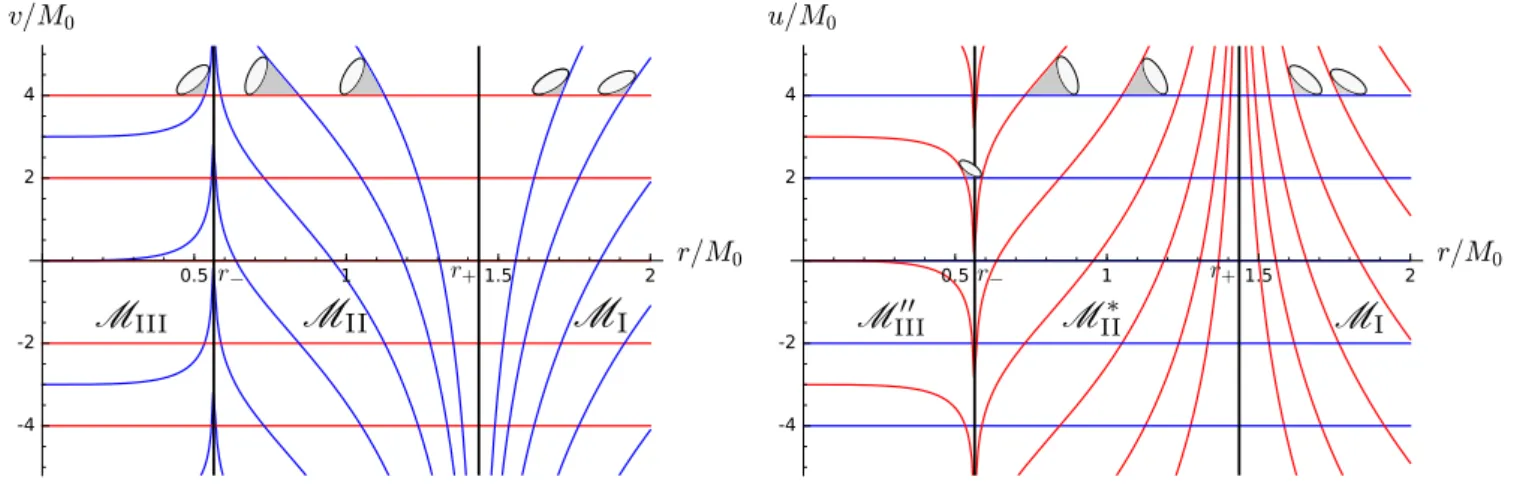
2.1 Location of the trapping horizons . . . 162

2.2 Hayward-like model . . . 163

2.3 Frolov’s model . . . 164

2.4 Bardeen-like model . . . 164

3 Behaviour of null geodesics in models with closed trapping horizons . . . 166

3.1 Null geodesic flow . . . 166

3.2 Frolov’s separatrix and quasi-horizon . . . 167

3.3 Relevant null geodesics for closed trapping horizons . . . 168

4 Towards a model for the formation and evaporation of a non-singular trapped region170 4.1 A form of the metric constrained by the energy-momentum tensor . . . 171

4.2 Explicit energy-momentum tensor . . . 172

4.2.1 Conditions on the energy-momentum tensor . . . 172

4.2.2 Generating a Hawking flux onI+ _{. . . 173}

4.2.3 Avoiding the NEC violation on_I− _{. . . 174}

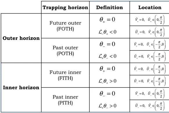
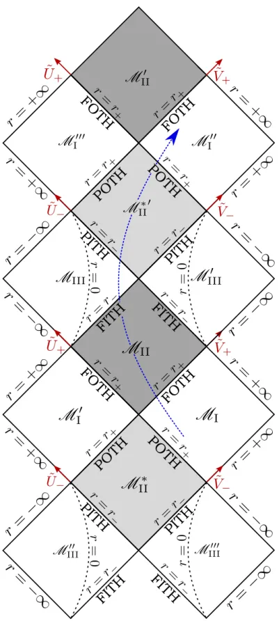
Conclusion 177 A Typology of horizons 179 1 Killing horizon . . . 179

2 Event horizon . . . 180

3 Trapping and apparent horizons . . . 180

3.1 Definition . . . 180

3.2 Dynamical spherically symmetric metric . . . 181

3.3 Stationary axisymmetric metric . . . 182

4 Cauchy horizon . . . 183

B Tensorial computations 185 1 General spherically symmetric metric . . . 185

2 Regular rotating black hole . . . 186

C Sagemath worksheets 189 1 Rotating non-singular black holes . . . 189

1.1 Curvature . . . 189

1.2 Null energy condition . . . 189

1.3 Geodesics . . . 189

1.4 Energy-momentum tensor from nonlinear electrodynamics . . . 190

I

NTRODUCTION

A

century after their discovery as a solution to Einstein’s equations, black holes are still at the heart of modern research in General Relativity. The seminal paper [104] by Karl Schwarzschild, providing the first vacuum solution to the equations of Einstein’s theory [49], does not explicitly mention the term “black hole” but paves the way for their explicit descrip-tion as regions of spacetime from which neither matter nor light can escape. In light of the recent experimental evidence in favor of their existence obtained thanks to the detection of gravitational waves [3], achieving a full grasp of the nature of these objects becomes an even more pressing matter.

Among the various fields of research dealing with black holes, the one we have explored in this thesis consists in better understanding the persistant question of the singularity lying at their center. The notion of singularity in gravitational physics has little to do with the meaning of the original Latin world singularitas, translating into “the fact of being unique”. However, the gravitational singularities we will be dealing with in this thesis do display a unique feature, as they appear to be predictions by General Relativity of its own limitations. One is for instance confronted with the presence of a singularity at the center of Schwarzschild’s black hole, where the curvature of spacetime diverges, which amounts to saying that spacetime itself cannot be defined there.

Singularity theorems, due to Penrose and Hawking [68,94], developed in the late 60’s and shed some light on the assumptions needed for the existence of such singularities, both for black holes and cosmology (in which one has to deal with the Big-Bang singularity). One of the key assumptions of these theorems is that matter should be well-behaved, in the sense that it oughts to satisfy some energy conditions. These conditions, and particularly the weakest of all, the null energy condition, can be violated when dealing with quantum phenomena. This fact tends to enforce the generally believed idea that a quantum theory of gravity would be able to cure singularities.

Since this theory has not yet been found, one is led to follow other approaches in order to study non-singular black holes reproducing Schwarzschild’s metric at large distance. The very first ex-ample of such model dates back to Bardeen’s black hole, proposed in 1968 [11]. Since then various other models have followed, among which some possessing a de Sitter core (Dymnikova [48] and Hayward [71]), and others inspired by non-commutative geometry (Nicolini [91]). These models all share a common feature: they introduce a new parameter in the black hole’s metric, preventing the curvature from diverging as r → 0. This might seem in contradiction with the no-hair theorem,

mass M, the reduced angular momentum a = J/M and the electric charge Q. Actually, there is no contradiction since the non-singular models are not solutions of vacuum Einstein’s equations.

As regards the approaches chosen to study non-singular black holes, pending for a theory of quantum gravity, this thesis aims at exploring two different ones. The first consists in considering modified theories of gravity. Starting from the Hamiltonian formulation of General Relativity, one can for instance add quantum corrections to it by hand (technically, by deforming the constraint algebra) in order to obtain effective Einstein’s equations, which might be a limit of the quantum Einstein’s equations from the fully quantized theory. Another option would be to work with modifed theories of gravity aiming at explaining the structure of the universe at large scale, in particular dark matter and dark energy, such as some scalar-tensor theories. We will show how one of these theories, namely mimetic gravity, could in principle allow recovering known non-singular black hole metrics.

The second approach assumes to stay inside the framework of General Relativity, but to match non-singular black hole metrics with exotic energy-momentum tensors. Non-linear electrodynam-ics, for instance, has been shown to be a potential source for some famous non-singular static black holes, such as Bardeen’s and Hayward’s. After constructing explicitly a regular rotating Hayward model, reducing to a regular rotating Hayward black hole in some regime and to Hayward’s static black hole in the absence of rotation, we will show that non-linear electrodynamics does not provide an adequate energy-momentum tensor anymore in this case. Finally, we will attempt to build a dynamical model for the formation and the evaporation of a non-singular black hole with an exotic energy-momentum tensor reducing to Vaidya’s solution in some regimes only.

In this thesis non-singular black holes are studied from quite various perspectives, ranging from their theoretical description to their observational consequences. At the interface lies the numerical simulations of the regular rotating Hayward model mentioned above. These simula-tions produce an image on the observer’s sky, i.e. a set of pixels to which is associated the specific intensity of a given photon. These images are computed by integrating backward in time the null geodesics, using the ray-tracing code GYOTO for which we developed an extension implementing the regular rotating Hayward model. Their comparison to typical Kerr black holes images will allow a better understanding of the forthcoming results of the Event Horizon Telescope currently observing the supermassive black hole candidate Sgr A∗ at the center of the galaxy.

This dissertation is organized as follows. The first chapter (Chap.1) deals with fundamentals of General Relativity, and aims at providing the reader with the essential ideas of General

Relativity as well as its main tools. Special attention shall be paid to the definition of singularities, and to the proof of Penrose’s 1965 theorem: the rest of the dissertation will be concerned with non-singular black holes, and the way they manage to circumvent Penrose’s theorem is to be highlighted for each of them. Chapter 2is the last introductive chapter, whose purpose is to present famous (singular) black hole solutions in General Relativity. Doing so we will come across several different notions of horizons, all summarized in App.A, the retained one to describe astrophysically relevant black holes being the trapping horizon. Our first encounter with non-singular black holes will occur in Chapter3, where we will present Bardeen and Hayward static black holes and then follow the first approach mentioned above, the one of modified gravity, to recover their metrics. Chapters4&5will be devoted to rotating non-singular black holes: we will present our regular rotating Hayward model, providing in its regime with horizons the first fully regular rotating black hole, and then compute with GYOTO the images we would observe if it were surrounded by an accretion structure similar to the one of Sgr A∗. Finally, Chapter6will deal with an attempt to model dynamical non-singular black holes describing the formation and evaporation of a non-singular trapped region.

C

H A P T E R

1

F

UNDAMENTALS OF

G

ENERAL

R

ELATIVITY

‘q_{∼n=j r}zh

˘.t rh˘∼n=j wz.t “Si je suis entré dans l’horizon, c’est que je connais le chemin !” (Textes des Sarcophages VII, 2w-2x, L2Li [30,43].)

T

he purpose of this first chapter1 is twofold. To begin with, we aim at giving an intuitive approach to Einstein’s general theory of relativity (Section1) . Furthermore, we develop the various relativistic tools that will be needed in the rest of this dissertation, which range from basic notions of differential geometry (Section2) to Einstein’s equations (Section3). This will lead us to define the notion of singularity in Section4and to give a formal proof of Penrose’s 1965 singularity theorem, hence setting the scene for the study of non-singular black holes in the next chapters. Finally, we will come across several notions of horizons, which are summarized in App.A.

Contents

1 Space, time and gravitation: from Galileo to Einstein . . . 6

2 Spacetime in General Relativity . . . 12 3 Einstein’s equations . . . 27 4 Singularity theorems . . . 31

1

Space, time and gravitation: from Galileo to Einstein

There is something unique about gravitation. It is the only force we know that couples identically to every massive object2. In other words, a feather and a billiard ball launched from the same height on the Moon will reach its surface simultaneously (since no other force than gravitation, like the friction of the atmosphere, applies there). This universality of free fall, already identified by Galileo in the 16thcentury, will lead us to consider gravitation not merely as a force but as an intrinsic property of spacetime. This spacetime is a paradigm in favour of which we will argue in Section1.1, before following Einstein and showing in Section1.2that gravitation is an expression of its curvature.

1.1 The fruitful union of space and time 1.1.1 Emergence of the notion of spacetime

At the 80thAssembly of German Natural Scientists and Physicians in 1908, Hermann Minkowski spoke about space and time in these terms:

“The views of space and time which I wish to lay before you have sprung from the soil of experimental physics, and therein lies their strength. They are radical. Henceforth, space by itself, and time by itself, are doomed to fade away into mere shadows, and only a kind of union of the two will preserve an independent reality.”

Evoking “the soil of experimental physics”, Minkowski was actually referring to the exper-iments of Albert Michelson and Edward Morley in the 1880’s. These experexper-iments aimed at measuring the speed of light from Earth in two opposite directions on a circular orbit around the Sun. At that time, light was thought to propagate in a medium called ether, which had a relative velocity with respect to Earth. Hence, the speed of light measured from Earth at two different points of its orbit, where it thus has two different relative velocities with respect to the ether, should vary.

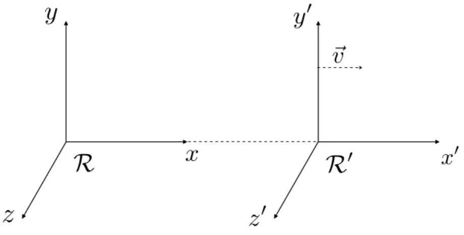
This fact simply stems from the Galilean transformations between two inertial frames of reference R and R0with relative velocity v (see Fig.1.1):

             t0_{= t} x0= x − vt y0_{= y} z0_{= z .} (1.1)

Michelson and Morley did not detect any difference between the two experiments performed at two opposite points of the Earth’s orbit, hence calling into question the theory of ether. This

1. SPACE, TIME AND GRAVITATION: FROM GALILEO TO EINSTEIN

x

y

z

R

R

0

x

0

y

0

z

0

~v

Figure 1.1: Illustration of two inertial frames,M and M0_{, with a velocity~v in the x direction relative to each other.}

led Einstein to postulate in 1905 that the speed of light3 c is the same in all inertial frames.

This postulate has dramatic consequences, as we shall see now. Let us consider a light ray bouncing back and forth on two mirrors, as illustrated in Fig.1.2. In the frame where the mirrors are at rest, after one bounce one has:

             ∆t =2L c , ∆x = 2L, ∆y = 0, ∆z = 0 (1.2)

The same situation seen in a frame where the mirrors are moving towards the right at a constant velocity v gives a quite different result. As illustrated in Fig.1.2, the distance travelled by the light ray from the point of view of an observer in R0is:

d = 2 s L2₊ µ∆x₀ 2 ¶2 (1.3) Following Einstein’s postulate, we now get

             ∆t0₌2 c q L2₊¡∆x0 2 ¢2 , ∆x0_{= v∆t}0_, ∆y0_{= 0,} ∆z0_{= 0} (1.4)

Combining the equations for∆t0_and∆x0_{, we obtain}

∆t0 ∆t = 1 q 1 −v_c22 ≡γ (1.5) 3

L

L

x0= v t0 A B A A B

Figure 1.2: Thought experiment illustrating the relativity of time. On the left panel, in a reference frameR, a light ray is bouncing back and forth vertically on two mirrors separated by a distance L. On the right, in a reference frameR0, the two mirrors are moving with a velocity~v in the x direction with respect to the frame of the left panel. Hence, a light ray travels a bigger distance A → B → A when the mirrors are moving (right). Since the speed of light is constant in all inertial frames, it means that the observer inR0will measure a bigger time interval∆t0than the one inR. Consequently, “time goes more slowly” in R0_.

Hence, the time interval measured in R0 is bigger than the one measured in R! We are forced to abandon the absolute vision of time stemming from Galileo’s transformations. The new transformations, known as Lorentz’s transformations, are:

             ct0=γ¡ ct −vx c ¢ x0_{=γ(x − vt)} y0_{= y} z0= z . (1.6)

They can be obtained by requiring that the interval ∆s2

= −c2∆t2+∆x2+∆y2+∆z2 (1.7)

remains invariant under such a transformation:∆s2₌∆s02. This simply enforces the fact that a light ray propagates at the same velocity c in all inertial frames.

The spatial and temporal components in Lorentz’s transformations (1.6) thus clearly get mixed up when going from an inertial frame to another, and two observers in these frames measure different times (if v is not too small compared to c, i.e. for relativistic motions). This mixing of space and time leads us to think the motion of observers in terms of a new paradigm, spacetime, that we will develop in the following section.

1.1.2 The spacetime of special relativity

If light propagates at the same velocity in all inertial frames, it must then be the highest possible one, i.e. all particles must travel at speed at most equal to c. This is easy to infer from the

1. SPACE, TIME AND GRAVITATION: FROM GALILEO TO EINSTEIN

Figure 1.3: Lightcone in Minkowski’s spacetime (with one less dimension of space). The event Q is on the future lightcone of O, while P is inside the lightcone. Finally, R is separated from O by a spacelike interval.LPis a timelike

curve, andLQis a null one.

invariance of the speed of light: for an observer moving at 0.99 c, a photon passing by will still travel at velocity c; the latter is thus an unsurpassable velocity.

The spacetime of special relativity, called Minkowski’s spacetime, is a 4-dimensional structure which enforces the invariance of the speed of light as well as its unsurpassable nature. It consists of a set of points, called events, characterized by four coordinates (t, x, y, z). Any two points are separated by the interval

∆s2_{= −∆t}2

+∆x2+∆y2+∆z2 , (1.8)

where, from now on, we set c = 1. When the points are infinitesimally close, this allows defining the line element

ds2_{= −dt}2_{+ dx}2_{+ dy}2_{+ dz}2, (1.9)

which, as we shall see in Sec.2.1.3, is associated with a metric which defines a notion of distance on the spacetime.

Hence, the separation of any two points∆s0 falls into one the three following categories : • ∆s2< 0: the interval is timelike

• ∆s2= 0: the interval is null • ∆s2> 0: the interval is spacelike

A curve is then said to be timelike (resp. null, spacelike) if every two points are separated by a timelike (resp. null, spacelike) interval.

Considering a point O in Fig.1.3, one can draw the light rays emerging from it, which satisfy ∆s2

= 0: this produces the lightcone at O, and in particular the null curve LQ. O is therefore

separated from the event Q by a interval, which means that the two can be linked only by a light ray. P is inside the future lightcone of O, the two points are separated by a timelike interval (∆s2< 0). It means that observers with velocities v < c can relate them. Finally, R is outside the future lightcone of O since they are separated by a spacelike interval (∆s2_{> 0): no observer can} go from O to R, for he would have to travel faster than light.

In the end, the spacetime structure gives a global coherent picture which enforces causallity. The future lightcone of O consists of all the events of spacetime that O can have an influence on, and it is preserved under Lorentz transformations. Put another way, all inertial observers, regardless the velocity they may have, will agree on the causal relation between two events separated by a timelike or null interval. This is not the case when the events are separated by a spacelike interval. For instance, two different observers could measure tR< tOand tR> tO.

1.2 Gravitation enters the game

Before getting into the formal description of General Relativity (Sec.2), let us introduce the main ideas of the theory.

1.2.1 Equivalence principles

We mentioned previously the universality of free fall highlighted by Galileo. It actually comes from the equality between the gravitational mass mg, associated with the weight P = mgg in

a gravitational field g, and the inertial mass mistemming from Newton’s second law F = mia

giving the force applied to an object to give it an acceleration a. When the only force applied to an object is gravity, assuming mi= mgone gets

a = g , i.e. d

2_x

dt2 = g (1.10)

Hence, the way a body falls in a gravitational field does not depend on its internal composition. Moreover, we can erase locally the effects of a static and uniform gravitational field by going to an accelerated frame: ( t0_{= t} x0_{= x −}1₂gt2 ⇒ d2x0 dt02 = 0 . (1.11)

1. SPACE, TIME AND GRAVITATION: FROM GALILEO TO EINSTEIN

Definition 1.1 (Weak equivalence principle). At each point of spacetime, in an arbitrary

gravita-tional field, one can define a locally inertial frame in a small enough region. In this frame, the motion of a free particle (i.e., only subject to gravity) is linear and uniform.

A classical illustration of the weak equivalence principle is the elevator in free fall. For an observer in such an elevator, all objects around him will fall at the same (increasing) speed. His frame of reference is thus a locally inertial frame, in which the motion of the objects surrounding him is linear and uniform.

Einstein extended this principle in the following way.

Definition 1.2 (Einstein’s equivalence principle). In the locally inertial frame of the weak

equiv-alence principle, all (non-gravitational) laws of nature are those of special relativity.

The notion of locally inertial frame is primordial here. Indeed, in the presence of a grav-itational field one cannot construct a global reference frame, otherwise the spacetime would be Minkoswki’s. It thus remains to define how to connect two different regions of spacetime with coordinates (xµ) and (x0µ), where two (independant) locally inertial frames can be constructed.

To do so, we will need an additional assumption: the laws of Physics do not depend on the specific choices of coordinates. In particular we require that the lightcone structure be preserved under a general transformation of coordinates xα→ x0α, i.e. ds2= ds02with:

ds2_{= gµν}dxµdxν_{= ds}02_{= g}0_αβdx0αdx0β (1.12)

Since the differentials dx0αare by definition dx0α₌∂x_∂x0αµdxµ, we get:

ds02= g0_αβ∂x 0α ∂xµdx µ∂x0β ∂xνdx ν _(1.13) Hence, we have g0_αβ= ∂x µ ∂x0α ∂xν ∂x0βgµν. (1.14)

The invariance of the line element ds2thus imposes a very specific constraint on the transforma-tion law of the metric. As will be shown in Sec.2.1.3, the metric is actually a covariant object, a tensor of type (0, 2), and thus transforms naturally as prescribed by eq. (1.14).

1.2.2 Gravity as a curvature of spacetime

The universal coupling of gravity, summarized in the weak equivalence principle, suggests that gravity is not merely a force but a property of spacetime itself. In this Section, we will give two ways of seeing that gravity is actually related to the curvature of spacetime.

A first hint at the presence of curvature can be directly inferred from Einstein’s equivalence principle. Indeed, let us make a coordinate transformation from a locally inertial frame with coordinates (Xµ) to a general frame with coordinates (xµ). The line element reads:

ds2_=ηµνdXµdXν. (1.15)

Generalizing eq. (1.11), the coordinate transformations to get to (xµ) are dXµ₌∂X_∂xαµdxα. Hence,

the line element can be rewritten:

ds2₌∂X µ ∂xα ∂Xν ∂xβηµνdx α_dxβ _{. (1.16)}

The coordinate transformation from (Xµ) to (xµ) can always be made, but the reverse cannot. Einstein’s equivalence principle implies that in the presence of gravity, any observer can go only locally from coordinates (xµ) to (Xµ), in which the line element takes the simple form (1.15). Such a transformation is thus not possible globally when gravity comes into play.

The line element thus takes a more complicated form in the presence of a gravitational field. But it encodes geometry, and can be seen in Minkowski’s spacetime as a generalization of the Pythagorean theorem. Hence, the presence of a gravitational field will lead to a modification of geometry, and to the presence of a nonvanishing curvature (which will be defined precisely in Section2.2).

Another, more explicit way of seeing this is through a thought experiment. Let us consider an accelerating rocket, in which a light ray is sent from the left wall to the right one. The light ray propagates in straight line, and during the time it needs to cross the rocket, the latter has accelerated. Hence, the light ray will reach the right wall at a smaller height than the one it was sent from: for an observer in the rocket, the acceleration has curved the light ray ! Via the Einstein equivalence principle, this acceleration is locally equivalent to a gravitational field. Hence, we can expect light rays to be curved in a gravitational field.

In the end, the gravitational field appears not to be an additional field of spacetime. It rather represents the deviation of the spacetime geometry from the Minkowskian flat geometry, and is materialized by the curvature of spacetime.

2

Spacetime in General Relativity

We have now written down the physical principles underlying the theory of General Relativity, but they remain to be implemented in a mathematical and practical framework. This is the aim of this section, where we will introduce the mathematical tools of the theory. They will prove necessary to understand the corner stone of GR, Einstein’s equations, as well as the singularity theorems, that we will develop in Secs.3&4.

2. SPACETIME IN GENERAL RELATIVITY

2.1 Manifolds and tensors 2.1.1 Manifolds

An essential notion in order to describe the spacetime of General Relativity is the one of a manifold. Intuitively, a manifold is a set of points linked in a continuous way and which locally looks likeRn, but perhaps not globally [6]. A natural example is the surface of the Earth which looks flat locally, but clearly not globally !

More precisely, we will be interested in manifolds on which we can make differential calculus, called differentiable manifolds. The easiest type of differentiable manifolds to work with is the smooth manifold, defined as follows.

Definition 1.3. A smooth n-dimensional4manifoldM is a topological space equipped with charts

ϕα:Uα→ Rn such that:

(i) U_αare a finite number of open sets coveringM , called an atlas,

(ii) the transition mapϕ_α◦ϕ−1_β :Rn_{→ R}nis smooth (i.e. C∞) whenU_{α∩ Uβ6= ;.}

Property (i) is at the heart of our intuitive definition of a manifold: locally, one can label the points p ∈ Uα⊂ M by n coordinates (xi) by using the chartϕ_α. But globally, one may need more that one open setU_αto cover the whole manifold.

Property (ii) allows defining unambiguously smooth functions f :M → R. f is smooth if for all

α, f ◦ϕ−1_α :Rn_{→ R is smooth (see Fig.}1.4_{). One can show that f is smooth on V = Uα∩ Uβ}using the chartU_{α: it suffices to show that f ◦}ϕ−1_α is smooth onϕ_{α(V ) ⊂ R}n. Thanks to property (ii), we arrive at the same conclusion by using the patchU_{β: if f ◦ϕ}−1

α is smooth onϕα(V ), then f ◦ϕ−1_β will be smooth onϕ_{β(V ) since f ◦}ϕ−1_{β = ( f ◦}ϕ−1_{α ) ◦ (}ϕ_α◦ϕ−1_β )

2.1.2 Tensors on manifolds

Now that we are equipped with a notion of manifold, we need to define various objects on it that will allow us to do some Physics. For instance, the notion of metric tensor, giving the concept of distance on a manifold, will be of the uttermost importance to define the spacetime of General Relativity.

A few steps are nonetheless necessary to get to the notion of tensors. Let us first define what a curve on a manifold is.

4

U

_β

U

_α

φ

_α−1

_f

!

!

n

M

f

!

φ

_α−1

V

Figure 1.4: Smooth n-dimensional manifoldM along with two of its charts UαandU_β. The open setsUαcovering M constitute an atlas. The function f : M → R is smooth iff f ◦ ϕ−1_{α is smooth for everyUαin the atlas.}

Definition 1.4. A (smooth) curve is a subsetL ⊂ M that is the image of a smooth map I ⊂ R → M :

P : I → R

λ7→ p = P(λ) ∈ L .

P is called a parametrization ofL , whileλis a parameter alongL .

One can also define a scalar field on a manifoldM as a function f : M → R. One can then define a vector tangent toL by applying it to f as follows.

Definition 1.5. A vector vvv tangent toL at p = P(λ) is an operator matching every scalar field f to the real number

vv_{v( f ) =} d f dλ ¯ ¯ ¯ ¯_L ≡ lim²→0 1 ²[ f (P(λ+²)) − f (P(λ))] (1.17)

One can define coordinates (xα_{) around p ∈ M , and thus n different curves Lα}going through p and parametrized by_{λ= x}α. This allows defining_∂∂∂α, the vector tangent toL_α, when a scalar field f is applied to it:

∂∂∂α( f ) = d f dxα ¯ ¯ ¯ ¯_L α = ∂f ∂xα (1.18)

2. SPACETIME IN GENERAL RELATIVITY

One can then rewrite any vector v applied to f as follows5 v v_{v( f ) =} ∂f ∂xα dXα dλ =∂∂∂α( f ) dXα dλ (1.19)

Since this is valid for all scalar fields f , we can decompose any vector as vv_{v = v}α_∂∂∂α, with vα=dX

α

dλ (1.20)

Definition 1.6. The set of all tangent vectors to a curve at p constitutes the tangent vector space

T_pM to M at p. The vectors_∂∂∂αform a basis of T_pM , and the coefficients vαare the components of vvv with respect to the coordinates (xα).

One can define linear forms on TpM as follows.

Definition 1.7. A linear form is a mappingω_{: v ∈ T}pM 7→ 〈ω, v〉 ∈ R that is linear: 〈ω, v + u〉 =

λ〈ω, v〉 + 〈ω, u〉 for all u, v ∈ TpM andλ∈ R.

Definition 1.8. The dual space of TpM , denoted by T∗pM , consists of all the linear forms at

p. Given the natural basis (∂_α) of TpM , there exists a unique basis (dddxα) of T∗pM such that

〈dddxα,∂_β〉 =δα_β.

We now have all necessary tools to define tensors on a manifold.

Definition 1.9. A tensor of type (k, l) at p ∈ M is a mapping T : T∗_pM × ··· × T∗_pM | {z } k times × TpM × ··· × TpM | {z } l times → R (_ω1, ··· ,ωk, v1, ··· , vl) 7→ T(ω1, ··· ,ωk, v1, ··· , vl).

that is linear with respect to each of its arguments.

According to this definition, vectors are simply tensors of type (1, 0) while linear forms are tensors of type (0, 1). Given a basis (e_α) of TpM and a dual basis (eα) in T∗pM , a tensor of type

(k, l) reads

T = Tα1···αk

β1···βleα1⊗ · · · ⊗ eαk⊗ e

β1_{⊗ · · · ⊗ e}βl_{. (1.21)}

2.1.3 The metric tensor

Let us now define precisely the metric tensor which generalizes the notion of distance on a manifold, and which will be essential to define curvature as well as the trajectories of observers in spacetime.

Definition 1.10. A pseudo-Riemannian metric tensor g on M is a tensor field obeying the

following properties:

(i) g is a bilinear form acting at each point p ∈ M on vectors in the tangent space: g(p) : (uuu,vv_{v) ∈} T_pM × T_pM → g(uuu,vvv) ∈ R,

(ii) g is symmetric: g(uuu,vv_{v) = g(vvv,u}uu),

(iii) g is non-degenerate: at any point p ∈ M , a vector uu_{u such that ∀vvv ∈ T}pM , g(uuu,vvv) = 0 is

necessarily the null vector.

How does this formal definition of tensors, and in particular of the metric tensor, relate to the one often used by physicists, characterizing them by the way they transform under coordinate changes? As we have seen in Section1.2.1, imposing that the light cone be invariant under general transformations of coordinates implies a condition on the metric:

g0_αβ= ∂x µ

∂x0α

∂xν

∂x0βgµν (1.22)

Let us check that this property stems from our definition1.9of tensors. As we shall see, it actually directly results from their multilinearity. Let us consider ggg as a (0, 2) tensor, i.e. a bilinear form (the precise definition of the metric tensor will be given in Section2.1.3, but is not needed for this argument), to which we apply the infinitesimal vector dx = dxα∂α= dx0α∂0_αexpressed in two different bases.

We have first:

g(dx, dx) = g(dxµ∂µ, dxν∂ν)

= g(∂µ,∂ν)dxµdxν by linearity of each argument = gµνdxµdxν

(1.23)

And with the vectors expressed in the prime basis:

g(dx, dx) = g(dx0α∂0

α, dx0β∂0β) = g(∂0_α,_∂0_β)dx0αdx0β = g0_αβdx0αdx0β

(1.24)

But the differentials dx0α are by definitions related to dxµ by dx0α₌∂x_∂x0αµdxµ. Hence, equating

(1.23) and (1.24) leads to:

g_µνdxµdxν_{= g}0_αβ∂x 0α ∂xµdx µ∂x0β ∂xνdx ν_{, (1.25)}

and finally, as expected:

g0_αβ= ∂x µ

∂x0α

∂xν

∂x0βgµν. (1.26)

In the bases where the metric is diagonal, it can be shown that it always has the same number s of negative (and thus (n − s) positive) components among (gαβ): this is the signature of the metric. When s = 0, g is called a Riemannian metric and is positive-definite. When s = 1, g is a

2. SPACETIME IN GENERAL RELATIVITY

Lorentzian metric.

We are now able to define the category of manifolds we will be dealing with in the subsequent chapters.

Postulate 1.1. The spacetime of General Relativity consists of a Lorentzian manifold, which is a

pair (M ,g) where M is a smooth manifold and g is a Lorentzian metric tensor on M .

How is it that Lorentzian manifolds are best suited for describing the spacetime of General Relativity? We can provide two answers to this question.

First, the metric is not positive-definitive: this allows implementing the finiteness of the speed of light and hence causality at each point of the manifold through the use of a light cone, which will not be changed under general transformations of coordinates. The trajectories of physical observers, necessary satisfying causality, are then timelike curves inside the light cone.

Furthermore, a Lorentzian manifold allows one to encode the equivalence principle. Indeed, let us consider a spacetime very different from Minkowski’s, for instance with some curvature (which will be defined properly in Section2.2). At a given point p, it will always be possible to define some inertial coordinates Xµsuch that the spacetime resembles Minkowski’s: g_{µν(p) =}η_µνand (_∂σg_µν)p= 0. This means, in total agreement with the equivalence principle, that one can locally

cancel the effects of gravity and place oneself in the frame of a freely-falling observer. Of course this is valid only locally, as emphasized by the expression of the metric in the neighbourhood of p:

g_µν=ηµν+1

2(∂σ∂ρgµν)pX

σ_Xρ_{+ · · · (1.27)}

The fact that one cannot impose that the second derivatives of the metric be null is precisely the manifestation of curvature.

2.2 Curvature

In this section, we will define the notion of curvature of a manifoldM in an intrinsic way, i.e. without requiring that there exist a higher-dimensional space in whichM may be embedded. A way of doing so consists in defining the parallel transport of tensors (Section2.2.1). The curvature can thus be characterized by parallel transporting them along a closed curve, via the Riemann tensor (Section2.2.2).

2.2.1 Levi-Civita connection on a manifold

What do we mean by parallel transport along a curve? This notion is best illustrated for vectors, where parallel transport boils down to transporting a vector while it keeps pointing in the same direction. In the usual Euclidean plane, the parallel transport along a closed curve is trivial as

1 2 3 4 p p 1 1 2 2 3 3 4 4

Figure 1.5: Parallel transport of a vector along a closed curve in a (flat) Euclidean plane (left) and on a (curved) sphere (right), following the path 1 → 2 → 3 → 4. Keeping the same direction all the way along, the vector on the sphere follows its curvature and has rotated after travelling along the loop, contrarily to the vector on the plane.

illustrated in Fig.1.5(left). Transporting the same vector along a closed curve on a 2-sphere (Fig.1.5_{(right)) is not as easy: at each point p ∈ S}2, the vector belongs to a different tangent space TpS2.

Hence we will need an additional structure on the manifold in order to compare vectors (and then tensors) belonging to different tangent spaces. The structure which allows defining the variation of a vector field vv_{v ∈ H (M ), hence providing a way of connecting various tangent spaces,} is called an affine connection.

Definition 1.11. An affine connection onM is a mapping

∇∇∇ : H (M ) × H (M ) → H (M ) (uuu,vv_{v) 7→ ∇∇∇uuu}vvv which satisfies the following properties:

(i) ∇∇∇ is bilinear

(ii) For any scalar field f ,

∇∇∇f uuuvvv = f ∇∇∇uuuvvv

(iii) For any scalar field f , the Leibniz rule holds: ∇

∇∇u( f vvv) = 〈∇∇∇ f ,uuu〉vvv + f ∇∇∇uuuvvv where ∇∇∇ f = ∂

f

∂xαdddx α

The vector ∇∇∇uuuvvv is called the covariant derivative of vvv along uuu. The affine connection can be

2. SPACETIME IN GENERAL RELATIVITY

same type as TTT.

An affine connection is entirely defined by its components Cµ_αβ. Its action on a basis (eee_α) at a given point reads:

∇

∇∇eeeβeeeα≡ C

µ

αβeeeµ (1.28)

We will use in the rest of this thesis a specific type of affine connection, the Levi-Civita connection, whose existence stems from the fundamental theorem of Riemannian geometry.

Theorem 1.1 (Fundamental theorem of Riemannian geometry). Let (M,g) be a pseudo-Riemannian

manifold. Then there exists a unique connection ∇∇∇, called the Levi-Civita connection, which satisfies (i) ∇∇∇ is torsion-free: for any scalar field f , ∇a∇bf = ∇b∇af

(ii) ∇∇∇ preserves the metric: ∇∇∇g = 0

The condition of preservation of the metric simply means that we require the connection to preserve the notion of distance, and in particular the structure of the lightcone. It implies the following form for the connection coefficients, which are the Christoffel symbols:

Cα_βγ=Γα_βγ≡1 2g

αλ¡

∂βgγλ+∂γgβλ−∂λgβγ¢ (1.29)

The absence of torsion means that the Christoffel symbols are symmetric with respect to their downstairs indices:

Γα_βγ=Γα_γβ (1.30)

Given a tensor field TT_{T of type (k, l), one can define the covariant derivative of ∇T}∇T∇T with respect to the affine connection ∇∇∇. It is a tensor field of type (k, l + 1) whose components are:

∇µTα1···αk_β1···βl ≡ (∇T∇T∇T)α1···αk β1···βlµ =∂µTα1···αk_β1···βl+ k X i=1 Γαi σµTα1··· ith_position ↓ σ···αk β1···βl− l X i=1 Γσ βiµT α1···αk β1···σ ↑ ithposition ···βl (1.31)

2.2.2 Riemann and Ricci tensors

Let us come back to Fig.1.5. Once the vector is parallelly transported around a closed curve on the sphere, it comes back rotated at the origin because of the curvature of the 2-sphere.

This notion of curvature can actually be encoded in the noncommutation of covariant deriva-tives applied to a vector:

where the Rδ_αβγare the components of the Riemann tensor. Computing explicitly the left-hand side of eq. (1.32) using eqs. (1.31) and (1.29) leads to the expression of the Riemann tensor:

Rd_abc≡∂bΓdac−∂cΓd_ab+Γace Γddb−Γ e abΓ

d

ec (1.33)

One can then define the Ricci tensor RRR (which is a contraction of the Riemann tensor) through its components:

R_{ab≡ R}c_acb (1.34)

And finally the Ricci scalar, also called scalar curvature, reads

R = Rabg

ab _(1.35)

Curvature scalars, i.e. scalars formed from the contraction of the Riemann tensor (or other tensors such as Weyl’s tensor), will be of the utmost importance in the following. Along with the Ricci scalar, the Kretschmann scalar K will often be computed in the following:

K = R_αβγδRαβγδ. (1.36)

Indeed, contrarily to tensors whose components depend on the choice of a specific basis, scalars are coordinate-independent. The divergence of the curvature scalars thus provides a way of characterizing singularities in spacetime, as will be explained in more details in Section4.

2.3 Geodesics

2.3.1 Geodesics’ equation

As previously mentioned, the particles which are subject solely to gravity play a peculiar role in General Relativity. They are associated with locally inertial frames, in which gravity is erased and the laws of special relativity are valid. Gravitation being described as a deformation of spacetime with respect to the flat geometry, it is natural to define the worldlines of these particles in free fall, called geodesics, as lines that "curve as little as possible" [122]. They will reduce to a straight line in a flat geometry, since inertial observers in Minkowski’s spacetime are at rest or in linear and uniform motion. The following definition encapsulates these properties.

Definition 1.12. A smooth curveL of a pseudo-Riemannian manifold (M , ggg) is called a geodesic

iff it admits a parametrization P whose associated tangent vector field vvv is transported parallelly to itself alongL :

∇∇∇vvvvvv = 0 (1.37)

Such a parametrization is called an affine parametrization of parameterλ. Recall that a smooth curve is the image of a smooth mapI → M (see Def.1.4). The parametrization is then

2. SPACETIME IN GENERAL RELATIVITY

defined by n functions Xα:I → R such that xα(P(λ_{)) = X}α(λ). In terms of components, the tangent vector is thus vα₌dX_dλα, where the (Xa) are the coordinates in the neighbourhood of a point p ∈ L . Hence, eq. (1.37) reads:

0 = vα∇αvβ = vβ∂v α ∂xβ+Γ α βγvβvγ = vvv(vα) +Γα_βγvβvγ by eq. (1.20) =dv α dλ +Γ α βγvβvγ by eq. (1.17) (1.38)

The geodesic equation thus reads:

d2Xα d2_λ +Γαβγ dXβ dλ dXγ dλ = 0 (1.39)

The interpretation of the geodesic equation is insightful and deeply rooted in the equivalence principle. Actually, ∇∇∇vvvvvv is the acceleration of a particle along the geodesic with velocity vvv. Hence,

the acceleration of a particle following a geodesic vanishes: no force is exerted on this particle, which is in free-fall. The inertial observers of General Relativity are those subject only to gravity. The curved structure of spacetime thus really takes into account the gravitational attraction, and does not treat it as a force.

2.3.2 Congruences of geodesics

A congruence of geodesics is a family of geodesics such that through each point of spacetime, there passes one and only one geodesic from this family. The geodesics among a given congruence are thus non-intersecting.

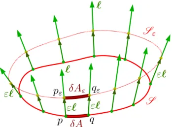
The expansion of a congruence of geodesics can be defined as the fractional change of area of a surface following the geodesics. Let us consider a codimension 2 surfaceS and a vector field lll associated with a congruence of light rays, also called null congruence (Fig.1.6). Let us take an infinitesimal parameter_{²> 0 and displace each point on S by the infinitesimal vector²}lll. This forms the new surfaceS_², and the resulting expansion ofS along lll is

θ(l)≡ lim

²→0

δA_²−δA

δA (1.40)

It can actually be shown that the expansion scalarθis independent of the choice ofS , and is a property of the geodesic congruence itself. In the rest of this dissertation, we will use the following definition of the expansion scalar:

Figure 1.6: Codimension 2 surfaceS and its image by a translation along the infinitesimal vector ²lll. Figure taken from [63].

which is equivalent to (1.40). hµνare the components of the induced metric hhh, defined via the two independent null vector fields lll and kk_{k (such that lll · kkk = −1):}

h

h_{h = ggg + lll ⊗ kkk + kkk ⊗ lll .} (1.42) Raychaudhuri’s equation describes the evolution of the expansion scalar. In the case of a congru-ence of null geodesics, the equation reads

dθ_(l) dλ = − 1 2θ 2 (l)−σ2+ω2− Rµνlµlν (1.43)

whereσis the shear scalar andωthe rotation parameter. This equation will prove essential in establishing Penrose’s singularity theorem in Sec.4.

2.4 Causal structure

This Section aims at giving a first approach to black holes and a way of representing them, namely Carter-Penrose diagrams.

2.4.1 Basic definitions

The metric tensor defined in Sec.2.1.3allows classifying vectors in terms of their causal nature.

Definition 1.13. A vector vvv belonging to the tangent space of a manifold equipped with a metric g

g

g of signature (− + ++) is • timelike if ggg(vvv,vv_{v) < 0 ,}