HAL Id: hal-01957173
https://hal.archives-ouvertes.fr/hal-01957173
Submitted on 17 Dec 2018
HAL is a multi-disciplinary open access
archive for the deposit and dissemination of
sci-entific research documents, whether they are
pub-lished or not. The documents may come from
teaching and research institutions in France or
abroad, or from public or private research centers.
L’archive ouverte pluridisciplinaire HAL, est
destinée au dépôt et à la diffusion de documents
scientifiques de niveau recherche, publiés ou non,
émanant des établissements d’enseignement et de
recherche français ou étrangers, des laboratoires
publics ou privés.
Optimal-Cost Reachability Analysis Based on Time
Petri Nets
Hanifa Boucheneb, Didier Lime, Olivier Henri Roux, Charlotte Seidner
To cite this version:
Hanifa Boucheneb, Didier Lime, Olivier Henri Roux, Charlotte Seidner. Optimal-Cost Reachability
Analysis Based on Time Petri Nets. 18th International Conference on Application of Concurrency to
System Design (ACSD 2018), Jun 2018, Bratislava, Slovakia. �hal-01957173�
Optimal-cost reachability analysis based on time
Petri nets
Hanifa Boucheneb
´
Ecole Polytechnique de Montr´eal, P.O. Box 6079, Station Centre-ville, Montr´eal, Qu´ebec, Canada, H3C 3A7
Didier Lime and Olivier H. Roux
´
Ecole Centrale de Nantes, 1, rue de la Noe – BP 92101 44321 Nantes Cedex 3, France {didier.lime,olivier-h.roux}@ec-nantes.fr
Charlotte Seidner
Universit´e de Nantes
2 avenue du Pr Jean Rouxel – BP 539 44475 Carquefou Cedex, France [email protected]
Abstract—This paper investigates the optimal-cost reachability problem in the context of time Petri nets, where a rate cost is associated with each place. This problem consists in deciding whether or not there exists a sequence of transitions reaching, with minimal cost, a given goal marking. This paper shows that for some subclasses of cost time Petri nets, the optimal-cost reachability problem can be solved more efficiently using a method based on the state classes, without resorting to linear programming or splitting state classes.
I. INTRODUCTION
Time Petri nets (TPNs for short) are a simple yet powerful formalism useful to model and verify real-time, concurrent systems that are therefore subject to time constraints. In TPNs, a firing interval, associated with each transition, specifies the minimum and maximum duration it must be maintained en-abled before its firing. Thus, TPNs can model time constraints, even when the exact delays or durations of events are not known. The verification of a TPN is based on the state space abstraction that takes into account the time constraints of the model, while preserving its markings and firing sequences.
This paper deals with the cost time Petri nets (cTPNs for short) and investigates the optimal cost reachability problem. A cTPN is a TPN extended with rate costs associated with its places. The rate cost of a place p is the sojourn cost (per time unit) of each token in place p. These rate costs do not affect the behaviour of the TPN but they allow to determine the sojourn cost in each marking and also the cost of firing a sequence of transitions.
The optimal cost reachability problem can be stated as the problem of deciding if there exists a sequence of transitionsω that allows to reach with minimal cost a given goal marking. Starting from the initial marking, the marking of the model evolves by firing transitions. Each time a transition is fired, some tokens are consumed and some others are produced. We define, for each transition t, a rate cost called incidence rate cost of t as the sum of rate costs of tokens produced by t minus the sum of rate costs of tokens consumed by t. We show that for sequences such that the incidence rate costs of their transitions are all non-negative or all non-positive, their optimal-costs can be computed more efficiently based on the state class method without using techniques of linear programming or decomposing state classes, as done
previ-ously. Moreover, we show how to compute the optimal-cost of sequences such that the firing interval of their transitions are all singular. Therefore, the optimal cost reachability problem can be solved more efficiently for some subclasses of cTPNs. Such subclasses might seem restrictive but can in fact model a wide range of applications. Consider for instance a leak in a pressure pipe: until its fixing, the rate at which the water leaks will surely increase, as the leak keeps getting larger. The subclass of model can also describe any economic system based on rarefying resources such as oil or Bitcoins, where the cost of things keep increasing.
The optimal-cost reachability problem has been addressed for Priced Timed Automata (PTAs for short) in [1]–[5] using the region graphs and the zone based graphs. In [1], the authors have proved the decidability of the optimal-cost problem for PTAs with non-negative costs. In [2]–[4], the computation of the optimal-cost to reach a goal location is based on a forward exploration of zones extended with linear cost functions. The linear cost function of a zone gives the optimal-costs to reach each state within the zone. In [5], the authors have improved the approach, developed in [2]–[4], so as to ensure termination of the forward exploration algorithm, even when clocks are not bounded and costs are negative, provided that the PTA is free of negative cost cycles.
For priced timed/time Petri nets, the optimal-cost reach-ability problem has been addressed in [6], [7]. In [6], the considered model is a timed arc Petri net, under weak firing semantics, extended with rate costs and firing costs associated with places and transitions, respectively. The computation of the optimal-cost for reaching a goal marking is based on similar techniques to those of PTAs [1]. In [7], the authors have investigated the optimal-cost reachability problem for time Petri nets where each transition has a firing cost and each marking has a rate cost (represented as a linear rate cost function over markings). To compute the optimal-cost to reach a goal marking, the authors have first revisited, to include costs, the state class graph method and then reduced the computation, as all other techniques, to a linear programming problem.
The rest of the paper is organised as follows. Section II is devoted to the TPN model, its semantics and its state class graph method. Section III presents the TPN extended with
costs considered here and then defines the cost of a run and the optimal-cost of a sequence. It also shows how to rewrite the cost of a run based on the incidence rate costs of its transitions. Section IV investigates efficient computation procedures of the optimal-cost of firing a sequence of transitions from a state class that need neither minimisation techniques nor splitting state classes. Section V shows by means of a case study how the optimal-costs are computed. Section VI concludes the paper by some future work.
II. TIMEPETRINETS
A. Definition and semantics
Syntactically, a time Petri net is a Petri net where a firing time intervals is associated with each transition.
Let N, Z, Q+ and R+ be the set of non-negative integers, the set of integers, the set of non-negative rational numbers and the set of non-negative real numbers, respectively. Let Q+[ ] be the set of non-empty intervals of R+ whose bounds are in Q+ and Q+∪ {∞}, respectively. For an interval I ∈ Q+[ ],↓ I and↑ I denote its lower and upper bounds, respectively.
Formally, a TPN is a tuple N = (P, T, pre, post, M0, Is)
whereP and T = {t1, ..., tm} (with m > 0) are finite sets of
places and transitions such that P ∩ T = ∅, pre and post are the backward and the forward incidence functions (pre, post : P × T −→ N), M0 is the initial marking (M0 : P −→ N),
andIs is the static firing interval function (Is : T → Q+[ ]). LetN = (P, T, pre, post, M0, Is) be a TPN, M : P −→ N
a marking andtia transition ofT . Transition tiis enabled for
M iff all required tokens for firing ti are present in M , i.e.,
∀p ∈ P, M (p) ≥ pre(p, ti).
In this paper, we use the original semantics of the TPN [8]: If a transition is multi-enabled in some state, only one instance of this transition is considered (single-server semantics), and when a transition is fired, all transitions disabled and enabled again, during this firing, are newly enabled.
We denoteEn(M ) the set of all transitions enabled for M , i.e., En(M ) = {ti∈ T | ∀p ∈ P, pre(p, ti) ≤ M (p)}.
If M results from firing some transition tf from some
marking, N w(M, tf) denotes the set of all transitions newly
enabled in M , i.e., N w(M, tf) = {ti ∈ En(M ) | ti =
tf∨ ∃p ∈ P, M (p) − P ost(p, tf) < pre(p, ti)}.
The TPN state is defined as a pairs = (M, I), where M is a marking and I is a firing interval function (I : En(M ) → Q+[ ]). The initial state of the TPN model is s0 = (M0, I0)
where I0(ti) = Is(ti), for all ti ∈ En(M0). The TPN state
evolves either by elapsing time or by firing transitions. When a transition ti becomes enabled, its firing interval is set to
its static firing interval Is(ti). The bounds of this interval
decrease synchronously with time, until ti is fired or disabled
by another firing. ti can fire if the lower bound of its firing
interval reaches 0 but must fire, without any additional delay, as far as any conflict avoids it, if the upper bound of its firing interval reaches0. The firing of a transition takes no time and leads to a new marking.
Let (M, I) and (M′, I′) be two interval states of the TPN model, θ ∈ R+ and t
f ∈ T . We write (M, I) θ
−→ (M′, I′),
also denoted (M, I) + θ, iff from state (M, I), we reach the state (M′, I′) by a time progression of θ units, i.e.,
∀ti ∈ En(M ), θ ≤ ↑ I(ti), M′= M and
∀tj∈ En(M′), I′(tj) = [M ax(↓ I(tj) − θ, 0), ↑ I(tj) − θ]
We write(M, I)−→ (Mtf ′, I′) iff from state (M, I), we reach
the state(M′, I′) by firing immediately the transition t f, i.e.,
tf ∈ En(M ), ↓ I(tf) = 0
∀p ∈ P, M′(p) = M (p) − pre(p, tf) + post(p, tf) and
∀ti∈ En(M′), I′(ti) =
(Is(ti) if ti∈ N w(M′, tf)
I(ti) otherwise.
We also use the abbreviation (M, I) θtf
−→ (M′, I′) for
(M, I)−→ (M, I) + θθ tf
−→ (M′, I′).
The TPN state space is the transition system (S, −→, s0),
wheres0is the initial state of the TPN andS = {s|s0 ∗
−→ s} (−→ being the reflexive and transitive closure of the relation∗ −→ defined above) is the set of reachable states of the model. A run in the TPN state space (S, −→, s0), starting from a
state s1, is a sequence σ = s1 θ1t1
−→ s2 θ2t2
−→ s3. . .. Sequences
θ1t1θ2t2. . . and t1t2. . . are the timed trace and the trace
(firing sequence) ofσ, respectively. A marking M is reachable iff ∃s ∈ S s.t. its marking is M . The runs of a TPN are all the maximal runs starting from its initial states0.
B. State class graphs
Among the TPN state space abstractions proposed in the literature, we consider here the state class graph (SCG) [9], [10]. A SCG state class α consists of a marking M and a conjunctionF of atomic constraints1
over the firing dates of the enabled transitions in marking M and the firing date, denoted by t0 of the transition leading to α. It represents
an over-approximation of the set of states reached by the same firing sequence from the initial TPN state. Note that for convenience purposes, firing delays in the classical SCG state classes in [9] are replaced by firing dates. The formulaF characterises the union of the firing date domains of all states withinα, reached by the same firing sequence from the initial state of the TPN.
The initial SCG state class of the TPN is the pair α0 =
(M0, F0), where M0 is the initial marking and F0 =
V
ti∈En(M0)
↓ Is(ti) ≤ ti− t0≤ ↑ Is(ti),
wheretiis a non-negative real valued variable representing the
firing date of the transitionti andt0 is a variable representing
the date ofα0, which is supposed to be0 for the initial state
class.
From the practical point of view, F is represented by a
Difference Bound Matrix (DBM in short) [11]. The DBM of F is a square matrix D, indexed by variables of F . Each entry
1An atomic constraint is of the form x− y ≤ c, where x, y are real valued
variables, c∈ Q ∪ {∞} and Q is the set of rational numbers (for economy of notation, we use operator≤ even if c = ∞).
dij represents the atomic constraint ti− tj ≤ dij. If there is
no upper bound on ti− tj withi 6= j, dij is set to∞. Entry
dii is set to 0. Although the same non-empty domain may be
encoded by different DBMs, they have a canonical form. The canonical form of a DBM is the representation with tightest bounds on all differences between variables, computed by propagating the effect of each entry through the DBM. A DBM can be seen as the matrix representation of a graph, called a constraint graph [12]. Its canonical form can be computed in O(n3), n being the number of variables in the DBM, using a shortest path algorithm, like Floyd-Warshall’s all-pairs shortest path algorithm [13].
Let CS be the set of all syntactically correct SCG state
classes andsucc a state class successor function: CS× T −→
CS∪ {∅}, defined by: ∀α = (M, F ) ∈ CS, ∀tf ∈ T ,
• succ(α, tf) 6= ∅ iff tf ∈ En(M ) and the following
for-mula is consistent (i.e., satisfiable):F ∧( V
t∈En(M)
tf ≤ t).
Intuitively, it means that tf is enabled in M and tf is
firable fromα before all other transitions enabled at M . In other words,tf is enabled inM and there is, at least,
a valuation of firing dates in F s.t. tf has the smallest
firing date.
• Ifsucc(α, tf) 6= ∅ then succ(α, tf) = (M′, F′), where:
∀p ∈ P, M′(p) = M (p) − pre(p, t f) + post(p, tf) and F′ is computed in 3 steps: 1) Set F′ to F ∧ ^ t∈En(M) tf ≤ t ∧ ^ t∈N w(M,tf) ↓ Is(t) ≤ t − tf≤↑ Is(t).
Notice that without loss of generality, for economy of notations, we suppose that the transitions of En(M ) are different from those newly enabled by transitiontf
from M .
2) Put F′ in canonical form2
.
3) Eliminate t0 and all variables associated with
transi-tions of CF(M, tf) − {tf} and rename tf int0.
Canonical forms make operations over DBMs much simpler [11]. Two state classes are said to be equal iff they have the same canonical form (i.e., they have the same marking and the DBMs of their formulas have the same canonical form). Note that, in the following, we will use indifferently (M, F ) or (M, D) to refer to the state class α, and we suppose that all DBMs are in canonical form. DBM canonical forms allow also to reduce the complexity of the firing rule as follows [10]. Let α = (M, D) be a state class and tf ∈ T a transition.
• tf is firable fromα iff
tf ∈ En(M ) ∧ ∀ti∈ En(M ), dif ≥ 0.
• If tf is firable from α then its successor state class
by tf is the state class α′ = (M′, D′), where M′ and
2The canonical form of F′is the formula corresponding to the canonical
form of its DBM.
the canonical form of the DBM ofD′ are computed as
follows: ∀p ∈ P, M′(p) = M (p) − pre(p, t f) + post(p, tf) and ∀ti, tj∈ En(M′), d′ i0= ↑ Is(ti) if ti∈ N w(M, tf), dif ifti∈ N w(M, t/ f), d′ 0j= −↓ Is(tj) if tj ∈ N w(M, tf), M in tu∈En(M) duj if tj ∈ N w(M, t/ f), d′ ij= 0 if i = j, M in(dij, d′i0+ d′0j) if i 6= j ∧ ti, tj∈ N w(M, t/ f), d′i0+ d′0j otherwise
III. COST TIMEPETRI NETS
A. Definition and semantics
A cost time Petri net (cTPN for short) is a time Petri net where a rate cost is associated with each place, giv-ing the sojourn cost per time unit of each token in that place. Formally, a Cost Time Petri Net is a tuple Nc =
(P, T, pre, post, M0, Is, r) where:
• N = (P, T, pre, post, M0, Is) is a TPN,
• r : P −→ Z is a rate cost function that associates a rate
cost with each place of the TPN.
Note that no cost is associated with the discrete firings of transitions; however, these costs can be added without affecting the results provided in this paper.
LetNc be a cTPN, t ∈ T a transition and M a marking of
the cTPN. We denote byrm(M ) the rate cost of M : rm(M ) =X
p∈P
M (p) × r(p).
The rate costs of places can be defined as in [7] by a linear function over markings. We define the incidence rate cost of t by:
rt(t) =X
p∈P
(post(p, t) − pre(p, t)) × r(p).
Intuitively, it represents the impact of firingt on the rate cost of a marking.
The semantics of a cTPNNc= (P, T, pre, post, M0, Is, r)
is the semantics of the TPN N = (P, T, pre, post, M0, Is).
However, the rate costs associated with places allow to com-pute different costs such as the costs of runs and the optimal costs of firing a sequence from a state or a state class ofN .
B. Cost of a run
Lets1= (M1, I1) be a state of Nc andσ = (M1, I1) θ1t1
−−→ (M2, I2) · · · (Mn, In)
θntn
−−−→ (Mn+1, In+1) a run of s1. The
cost ofσ is defined by: Cost(σ) =
n
X
i=1
Let τ0 the date at which the state s1 is reached and
τj = τ0+ j
P
i=1
θi be the firing date of the transition tj in σ,
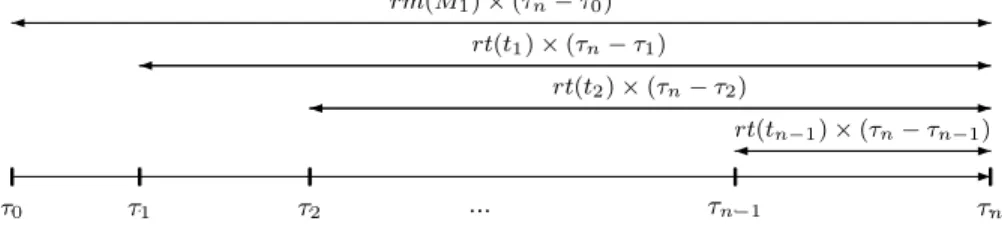
forj = 1, n. Proposition 1 rewrites Cost(σ) by means of the firing dates and incidence rate costs of transitions of σ (see Fig. 1). As we will show, this form is more useful to deal with the optimal-cost problem in some cases. The optimal-cost of Cost(σ) can be also rewritten by means of the firing dates and the rate costs of markings as shown in Proposition 2.
Proposition 1: Cost(σ) = rm(M1) × (τn− τ0) + n−1 X j=1 rt(tj) × (τn− τj).
Proof: By definition,Cost(σ) =
n
P
i=1
(θi× rm(Mi)). For
i = 2, n, the rate cost of the successor marking MiofMi−1by
tiisrm(Mi) = rm(Mi−1)+rt(ti−1). Therefore, for i = 2, n,
rm(Mi) = rm(M1) + i−1 X j=1 rt(tj). Then: Cost(σ) = θ1× rm(M1) + n X i=2 (θi× (rm(M1) + i−1 X j=1 rt(tj))).
It can be developed and rewritten as follows: θ1× rm(M1)+
θ2× (rm(M1) + rt(t1)) + ....+
θn× (rm(M1) + rt(t1) + rt(t2) + .... + rt(tn−1)).
Finally, Cost(σ) can be rewritten so as the rate cost of M1
(i.e., rm(M1)) is the coefficient of n
P
i=1
θi, the incidence rate
cost oft1(i.e.,rt(t1)) is the coefficient of n
P
i=2
θi, ..., and so on,
the incidence rate cost oftn−1(i.e.,rt(tn−1)) is the coefficient
ofθn. It follows that: Cost(σ) = rm(M1) × ( n X i=1 θi) + n−1 X j=1 rt(tj) × ( n X i=j+1 θi).
To achieve the proof, it suffices to replace
n P i=1 θi withτn− τ0 and n P i=j+1 θi withτn− τj. Proposition 2: Cost(σ) = ( n−1 X i=1 −rt(ti) × τi) + rm(Mn) × τn.
Proof: By definition,Cost(σ) =
n P i=1 (θi× rm(Mi)). For i = 1, n, θi= τi− τi−1. Then: Cost(σ) = n X i=1 ((τi− τi−1) × rm(Mi)).
Fori = 1, n − 1, the rate cost of the successor marking Mi+1
ofMi byti isrm(Mi+1) = rm(Mi) + rt(ti). Therefore, for
i = 1, n − 1, rt(ti) = rm(Mi+1) − rm(Mi). The previous
expression of Cost(σ) can be developed and rewritten as follows: ( n−1 X i=1 (rm(Mi) − rm(Mi+1) × τi) + rm(Mn) × τn.
To achieve the proof, it suffices to replace rm(Mi) −
rm(Mi+1) with −rt(ti).
C. Optimal cost of a firing sequence
Letα1be a state class ofNcandρ = α1 t1
−→ α2· · · αn tn
−→ αn+1a path ofα1,ω = t1· · · tn andΠ(α1, ω) the set of runs
ofα1that support the same sequence of transitionsω and lead
to states of α = αn+1. The optimal-cost of firing ω from α1
(or the optimal-cost ofρ) is:
OptCost(α1, ω) = M in σ∈Π(α1,ω)
Cost(σ).
The optimal-cost of firing ω from α1 can be computed
by extending state classes with costs and using linear programming techniques as in [7].
D. Optimal-cost reachability problem
The classical forward exploration algorithm in [2]–[4], [7] is adapted in Algorithm 1 to compute the optimal-cost to reach, from the initial marking, a marking belonging to a given set of markingsGoal. For each state class α such that its marking is in Goal, its optimal-cost is computed and compared with M inCost, where the smallest cost computed so far is saved. As usual, the lists P assed and W aiting are used to store the already processed and not yet processed state classes, respectively. The notation ω ≺ ω′ means that ω is a prefix
ofω′.
For bounded TPNs with no negative cost cycles, the algo-rithm terminates as for infinite sequences only finite prefixes, yielding the longest elementary paths, are explored.
In the following sections, we investigate cases where the optimal-costs of firing sequences can be computed without splitting state classes nor using linear programming tech-niques.
IV. COMPUTING OPTIMAL COST OF FIRING SEQUENCES
Letα1= (M1, F1) be a state class of Nc andρ = α1 t1
−→ α2· · · αn
tn
−→ αn+1a path ofα1andω = t1· · · tn. For ease of
notation, we suppose that all transitions within En(M1) and
those enabled by every transition of ω are all different. The firing date domain of transitions ofω from α1can be retrieved
by modifying the firing rule given in Section II-B. Indeed, it suffices, in step 3 of succ(αi, ti), for i ∈ [1, n], to keep ti.
More precisely replace step 3 with: Eliminate all variables associated with transitions of CF(Mi, ti) − {ti}. With this
modification, each variable ti, for i ∈ [1, n], represents the
firing date of the ith transition ofω. The variable t 0 is the
τ1 τ2 ... τn−1 τn τ0 rt(t2) × (τn− τ2) rm(M1) × (τn− τ0) rt(tn−1) × (τn− τn−1) rt(t1) × (τn− τ1)
Fig. 1. The cost of the run σ based on the firing dates and incidence rate costs of its transitions
Algorithm 1 Symbolic algorithm for optimal-cost reachability problem
1: M inCost ← ∞ 2: P assed ← ∅
3: W aiting ← {((M0, D0), ǫ)} 4: whileW aiting 6= ∅ do
5: select((M, D), ω) from W aiting
6: ifM ∈ Goal and OptCost((M0, D0), ω) < M inCost
then
7: M inCost ← OptCost((M0, D0), ω) 8: end if
9: if (for all ((M′, D′), ω′) ∈ P assed, ((M′, D′) 6=
(M, D)) or ¬(ω′≺ ω)) then 10: add((M, D), ω) to P assed
11: for all t ∈ F r(M, D), add (succ((M, D), t), ωt) to W aiting
12: end if
13: end while
14: return M inCost
date when α1 is reached. Let F G be the resulting formula.
The firing date domain of transitions of ω from α1 is the
projection of the domain ofF G to ti fori ∈ [0, n].
A. Case of non-negative incidence rate costs
For this section, we suppose that the incidence rate costs of all transitions of ω, except the last one are non-negative and rm(M1) ≥ 0. We will show that, under these assumptions,
to compute the optimal-cost of firing ω from α1, we need to
keep track of the minimal delay between the previously fired transitions and the coming ones, including the current one. But we do not need to retrieve delays between the previously fired transitions. Consequently, the relevant part of F G needed to compute the optimal-costs can be represented by a DBM of order(|ω| + 1) × |En(M ) ∪ {tn}|.
We denote by G the DBM in canonical form of order (|ω| + 1) × |En(M ) ∪ {tn}| defined by
∀i ∈ [0, |ω|], ∀tj ∈ En(M ) ∪ {tn}, gij = M ax(ti− tj|F G).
Since ti − tj ≤ 0, the value −gij is the minimal delay
between the firing datestj andti. Note thatG is a sub-matrix
of the DBM in canonical form ofF G. The size of the DBM ofF G is (|ω| + 1 + |En(M )|)2. Theorem 1: OptCost(α1, ω) = −g0n× rm(M1) + n−1 X i=1 rt(ti) × −gin.
Proof: Let GG be the DBM in canonical form of F G. Recall that G is a sub-matrix of GG. To achieve the proof, we first show that the valuationvi= gin− g0n fori ∈ [1, n]
is a feasible firing schedule for ω, i.e., for i, k ∈ [1, n], −gg0i≤ vi ≤ ggi0andvi− vk≤ ggik.
By definition, for i ∈ [1, n], vi = gin− g0n = ggin− gg0n,
then fori, k ∈ [1, n], vi−vk = gin−gkn= ggin−ggkn. Since
GG is in canonical form, it holds that ggin ≤ ggi0+ gg0n,
gg0n≤ gg0i+ ggin, and ggin≤ ggik+ ggkn. It follows that
−gg0i≤ vi ≤ ggi0andvi− vk≤ ggik.
The run corresponding to this firing schedule ofω is shown in Fig. 2. Its cost is:
−g0n× rm(M1) + n−1
P
i=1
rt(ti) × −gin.
By assumption,rm(M1) ≥ 0 and for i ∈ [1, n−1], rt(ti) ≥ 0.
Furthermore, fori ∈ [0, n], −ginis the minimal value oftn−ti
in F G, where tn is the firing date of last transition of ω.
Therefore,OptCost(α1, ω) = −g0n× rm(M1) + n−1 X i=1 rt(ti) × −gin.
According to the definition of G, for ω = ǫ, G is a DBM of order 1 × (|En(M )| + 1) defined by ∀tj ∈ En(M ) ∪ {t0}, g0j = d0j. Let us show now how
to compute progressively the DBMG of a nonempty sequence.
Proposition 3:Letα be the state class reached by a path ρ, G the corresponding DBM and tf a transition firable fromα
andα′ = (M′, D′) = succ(α, t f).
Then, the DBMG′ of the pathρ tf
−→ (M′, D′) is the DBM in
canonical form of order(|ωtf|+1)×|En(M′)∪{tf}| defined
by:∀i ∈ [0, |ωtf|] and tj ∈ En(M′) ∪ {tf}, gij′ =
M in(gij, gif+ d′0j) if i ≤ |ω| ∧ tj6∈ N w(M, tf) gif+ d′0j if i ≤ |ω| ∧ tj∈ N w(M, tf) d′ 0j if i = |ωtf| whered′ 0j = M in tu∈En(M) duj, if tj ∈ N w(M, t/ f) and d′ 0j= − ↓ Is(tj), otherwise.
Proof: The proof is based on the constraints added to computesucc(α, tf). Indeed, the firing condition is obtained
by adding toD, the constraints: tf ≤ tu, fortu∈ En(M ) and
Notice that all the added constraints involve tf and in
the corresponding constraint graph, they are represented by arcs (tf, tu, 0), for tu ∈ En(M ), (tj, tf, ↑ Is(tj)) and
(tf, tj, −↓ Is(tj)), for tj∈ N w(M, tf).
Therefore, the shortest path connecting a node ti, for i ∈
[0, |ωtf|], to a node tj ∈ En(M′) is:
M in(gij, gif+ M in tu∈En(M)
duj), if tj6∈ N w(M, tf) and
gif− ↓ Is(tj), otherwise.
By the firing rule given in II-B, it holds that: d′ 0j = −↓ Is(tj) iftj∈ N w(M, tf), M in tu∈En(M) duj iftj∈ N w(M, t/ f), Note that, M in tu∈En(M) duf = 0 as tf is firable. Consequently, g′if = gif, fori ∈ [0, |ωtf|].
Fori = |ωtf|, gij′ = d′0j asg′ij is the smallest path connecting
tf totj.
The computation of the optimal-cost of firing ω from α1
needs to carry in the DBMG the minimal firing delay between each fired transition ofω and the coming ones, including the current one. Thus, the size of G grows with the size of ω: indeed, the optimal-cost ofωtf is reached whentf is fired as
soon as possible (i.e.,−gnf = −d0f) fromα and the previous
ones are fired as late as possible (i.e., −gif) without causing
any delay to tf. It means that, to retrieve the firing schedule
yielding the optimal-cost of ω, the firing dates of its previous transitions need to be updated to take into account the fact thattf is fired as soon as possible and the previous ones are
fired as late as possible but before tf.
However, for bounded TPNs with no negative cost cycles, each infinite sequenceω′′ ofN
c, has some prefixω followed
by a repetitive sequence ω′ that loops on a state class α
reachable from the initial state class α0 byω. It follows that
OptCost(α0, ω) ≤ OptCost(α0, ω′′) and OptCost(α, ω′) ≤
OptCost(α, ω′k), for k ≥ 1. The cost of a cycle is
non-negative, if the sum of the incidence rate costs of all its transitions is non-negative and the rate cost of one of its marking is non-negative. This sufficient condition guarantees for a cycle a non-negative cost.
In the following, we investigate the possibility to reduce the size of the DBM G.
B. Memoryless state classes w.r.t. optimal-costs
Let α = (M, D) be the state class reached by a sequence ω from a state class α1 ofN . The state class α is said to be
memoryless w.r.t. optimal-costs iff for each sequenceω′ ofα,
OptCost(α1, ωω′) = OptCost(α1, ω) + OptCost(α, ω′)
Therefore, for any state classes α1 and α′1 leading by
sequences ω and ω′, respectively, to the same memoryless
state class α = (M, D) w.r.t. optimal-costs, it holds that for each firable sequence ω′′ fromα,
OptCost(α1, ω) ≤ OptCost(α′1, ω′) ⇒
OptCost(α1, ωω′′) ≤ OptCost(α′1, ω′ω′′)
Lemmas 1 and 2 provide two different sufficient conditions for the state class α to be memoryless w.r.t. optimal-costs. The first one depends on the DBM G of ω. The second one depends onα.
Lemma 1: Let α = (M, D) be the state class reached by some sequenceω = t1· · · tnfrom a state classα1= (M1, D1)
andG the DBM of its firing domain.
If ∀i ∈ [0, |ω|], ∀tj ∈ En(M ), gij = gin+ d0j then, α is
memoryless w.r.t. optimal-costs.
Proof: Suppose that ∀i ∈ [0, |ω|], ∀tj ∈ En(M ), gij =
gin + d0j. Let us show that for every sequence ω′ of α,
OptCost(α1, ωω′) = OptCost(α1, ω) + OptCost(α, ω′). We
consider 2 cases: 1)ω = t1...tn andω′= tj, and
2)ω = t1...tn and|ω′| > 1.
1) Case ω = t1...tn andω′ = tj: Since ∀i ∈ [0, |ω|], g′ij =
gin+ d0j. Consequently, if tj is firable fromα = (M, D) then
the optimal-cost of the successor ofα by tj is:
OptCost(α1, ω) + (rm(M1) + X i∈[1,|ω|] rt(ω(ti))) × −d0j. Note that rm(M ) = rm(M1) + P i∈[1,|ω|] rt(ω(ti)) and
rm(M ) × −d0j is the optimal-cost of firing tj from (M, D).
2) Case ω = t1...tn and |ω′| > 1: Suppose that in the
DBM G′ of ω′ from α, ∀t
j ∈ En(M′), g′ij = gin + cj,
where cj does not depend on i and is the opposite of the
minimal delay between firing dates of tj and tn. Let us
show that in any extended sequence of ω′ by any firable
transitiontk leading to the state class(M′′, D′′), it holds that
∀tj ∈ En(M′′), gij′′ = gin+ c′j, where c′j does not depend
on i and is the opposite of the minimal delay between firing dates oftj andtn, andG′′ is the DBM of the extended path.
By Proposition 3,∀tj∈ En(M′′) ∪ {tn}, iftj6∈ N w(M′, tk) then, g′′ij= M in(gij′ , g′ik+ M in tu∈En(M′) d′uj) = gin+ M in(cj, ck+ M in tu∈En(M′) d′uj). Otherwise, gij′′ = g ′ ik− ↓ Is(tj) = gin+ ck− ↓ Is(tj). Then,g′′
ij = gin+ c′j, wherec′j does not depend oni and c′j is
the opposite of the minimal delay between the firing dates of tj andtn(the proof of this claim is similar to the one provided
for Proposition 3). Therefore, the optimal reachability cost of any extended sequenceωω′ofω is the sum of OptCost(α
1, ω)
and the optimal cost of firingω′fromα (i.e., OptCost(α, ω′)).
Lemma 2: Let α = (M, D) be a state class such that all transitions of En(M ) are newly enabled in M . Then, α is memoryless w.r.t. optimal-costs.
t1 t2 ... t n−1 tn t0 −g2n −g0n −g(n−1)n −g1n
Fig. 2. The run corresponding to the firing schedule vi= gin− g0n, for i∈ [1, n], of ρ
Proof: Suppose that α is reached from some state class α1 by a sequenceω = t1· · · tn and G the DBM of its firing
domain. As all transitions of α are newly enabled, it follows that ∀i ∈ [0, |ω|], ∀tj ∈ En(M ), gij = gin+ d0j. According
to Lemma 1, α is memoryless w.r.t. optimal-costs.
Thanks to lemmas 1 and 2, when a memoryless state classα w.r.t. optimal-costs is reached, there is no need to explore its successors, in case there is in the list P assed an identical memoryless state class with smaller optimal-cost. Among the identical memoryless state classes reached by different paths, the one with the smallest optimal-cost will yield the optimal reachable cost, for all state classes reachable from α. Therefore, Algorithm 1 can be improved for this subclass of cTPNs.
C. Case of non-positive incidence rate costs
For this section, we suppose that the incidence rate costs of all transitions of ω, except the last one, are non-positive andrm(Mn) ≥ 0. Theorem 2: Let ρ = α1 = (M1, D1) t1 −→ α2 = (M2, D2) · · · αn = (Mn, Dn) tn −→ αn+1 = (Mn+1, Dn+1)
be a path in the SCG of Nc, supporting the sequence ω =
t1· · · tn. LetGG be the DBM in canonical form of F G (the
firing domain transitions ofω and those enabled in Mn). Then,
OptCost(α1, ω) = ( n−1
X
i=1
rt(ti) × gg0i) − gg0n× rm(Mn).
Proof: We first show that the valuationvi = −gg0i for
i ∈ [1, n] is a feasible firing schedule for ω, i.e., for i, k ∈ [1, n], −gg0i≤ vi≤ ggi0 andvi− vk≤ ggik.
By definition, fori ∈ [1, n], vi= −gg0i, then fori, k ∈ [1, n],
vi−vk = gg0k−gg0i. SinceGG is in canonical form, it holds
that gg0k ≤ gg0i+ ggik. It follows that −gg0i ≤ vi ≤ ggi0
andvi− vk≤ ggik.
By assumption,rm(Mn) ≥ 0 and for i ∈ [1, n−1], rt(ti) ≤ 0.
Furthermore, for i ∈ [0, n], −gg0i is the minimal value of ti
inF G (i.e., the firing date of the ith transition of ω).
By Proposition 2, the cost of each run supporting the sequence ω is: ( n−1 X i=1 −rt(ti) × τi) + rm(Mn) × τn. Therefore,OptCost(α1, ω) = ( n−1 X i=1 rt(ti) × gg0i) − rm(Mn) × gg0n.
D. Case of singular intervals
For this section, we suppose that the firing intervals of all transitions of ω are singular but the incidence cost rate of each transition ofω is negative, null or positive.
Theorem 3: Let ρ = α1 = (M1, D1) t1 −→ α2 = (M2, D2) · · · αn = (Mn, Dn) tn −→ αn = (Mn+1, Dn+1) be a
path in the SCG ofNc, supporting the sequenceω = t1· · · tn.
Then, OptCost(α1, ω) = n X i=1 −di0i× rm(Mi). Proof: The cost of each run σ = (M1, I1)
θ1t1 −−→ (M2, I2) · · · (Mn, In) θntn −−−→ (Mn+1, In+1) supporting ω is: n X i=1 (θi× rm(Mi)).
The domain of each θi, for i ∈ [1, n], [−di0i, dii0]. As
the firing interval of all transitions of ω are singular, each transition is fired at an exact date. Therefore, for i ∈ [1, n], −di0i= dii0.
V. CASE STUDY
In the French academic system, faculty positions with both teaching and research activities can be held either by an associate professor (maˆıtre de conf´erences, or MCF) or by a full professor (professeur des universit´es, or PU). In this system, a typical career path is:
• start as an associate professor at the 1st grade (´echelon 1);
• get promoted to higher grades; such promotions are automatic and usually3 happen every 34 months (that is, 2 years and 10 months after the last promotion);
• after some years, defend a habilitation thesis and obtain a higher degree (known as the habilitation `a diriger
des recherches), a qualification needed to supervise PhD students;
• depending on the opportunities, get a promotion from
associate to full professor; keep getting automatic pro-motions to higher grades according to seniority4.
To each grade corresponds an indice (a salary scale grade), on which the salary is based; additionally, when promoted from associate to full professor, the indice cannot decrease.
Let us consider the case of an associate professor who reaches the 4th ´echelon when 32 years old. Let us further
3For some reason, the switch from 1st to 2nd grade only takes 12 months,
whereas the switch from 6th to 7th takes 42 months (3 years and 6 months).
suppose that the university wishes that all faculty members become full professors and reach the last grade by the time they are 55. Obviously, the cheapest way for the university to reach this goal is to promote anyone at the latest possible time: given the durations between grades, this means letting the person reach the 9th grade after 14 years and 10 months; keep them in that grade for 2 years and 8 months; promote them to full professor and let them reach the last grade after 5 years and 6 months.
However, this strategy does not take into account the frus-tration of the person, which increases each time a promotion is denied, starting from the moment they reach the 6th grade and begin questioning their life choices.
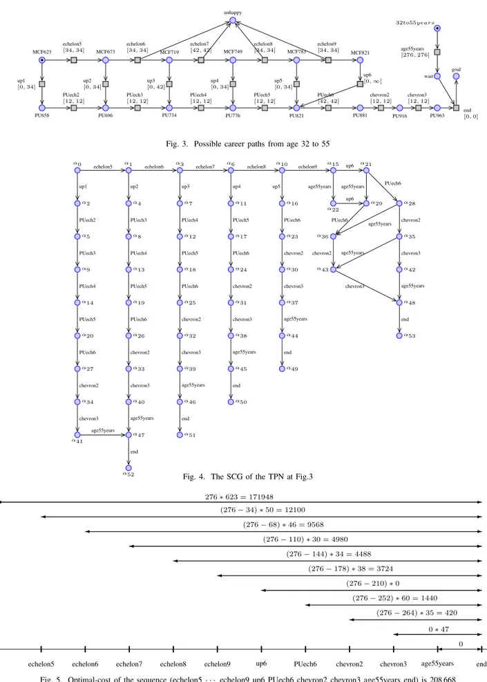
We propose a model for this optimisation problem, shown in Fig. 35. Each place with a M CF xyz label corresponds to a grade in the associate professor scale; its rate cost is equal to xyz (and is actually equal to the indice for this grade). Similarly, each place with a P U xyz label corresponds to a grade in the full professor scale. In the following, we give various values toR = r(unhappy) so as to show the interest of our method; the rate cost of all the other places is set to 0. The state class graph of the model is depicted in Fig.4 and Table I; note that a total of 10 paths in the SCG lead to a marking where goal contains 1 token; in the following, we denoteGoal the set of such markings.
To keep the model simple enough, it should be noted that it does not guarantee that the placegoal is attained when the person is exactly 55 years old (a token could stay in place wait for more than 0 time unit, for instance). However, we can show that, in the following, all optimal-cost strategies are such that the place goal is attained as early as possible, that is, after 23 years.
Let us first setR = 0. The optimal cost of each path leading to a marking in Goal is given in Table II and the minimum is equal to 208 668. The computation steps of this cost are re-ported in Fig.5: as expected, the optimal strategy is to give the promotion at the latest possible time, thus leading to the fol-lowing timed trace6:echelon5@34, echelon6@34, echelon7@42, echelon8@34, echelon9@34, up6@32, PUech6@42, chevron2@12, chevron3@12, age55years@0, end@0.
Let us now change the value of R; whenever R ≤ 32, the optimum strategy remains the same. For R = 33, the strategy consists in giving the promotion not too early, just before switching from 6th to 7th grade. The timed trace, with a total cost of 228 480, is:echelon5@34, echelon6@34, up3@42, PUech4@12, PUech5@12, PUech6@42, chevron2@12, chevron3@12, age55years@76, end@0.
Whenever R ≥ 34, the strategy consists in giving the promotion just before risking unhappiness, that is right before switching from 5th to 6th grade. ForR = 35, the computation steps are reported in Fig.6 and the timed trace, with a total cost
5Note that, keeping in tune with the French spirit, unhappiness keeps
building up and that even after getting a promotion from associate to full professor, the resentment is such that the unhappiness level is maintained.
6For the sake of legibility, we denote t
1@θ1, t2@θ2. . . the sequence
θ1t1θ2t2. . .
of 228 660, is:echelon5@34, up2@34, PUech3@12, PUech4@12, PUech5@12, PUech6@42, chevron2@12, chevron3@12, age55years@106, end@0.
VI. CONCLUSION
This paper deals with the optimal-cost reachability problem in the context of time Petri Nets extended with costs (cTPNs). It establishes, for some interesting subclasses of cTPNs, ef-ficient algorithms that compute the optimal-cost of firing a sequence of transitions from a given state class. Unlike the approaches developed in [1]–[7], the algorithms, presented here, are not based on techniques of linear programming. Finally, a case study is provided to show the interest of the proposed method.
As a future work, we will investigate the optimal-cost reachability problem in the context of parametric cTPNs.
REFERENCES
[1] R. Alur, S. L. Torre, and G. J. Pappas, “Optimal paths in weighted timed automata,” Theoretical Computer Science, vol. 318, no. 3, pp. 297 – 322, 2004. [Online]. Available: http: //www.sciencedirect.com/science/article/pii/S0304397503005838 [2] G. Behrmann, A. Fehnker, T. Hune, K. Larsen, P. Pettersson, J. Romijn,
and F. Vaandrager, Minimum-Cost Reachability for Priced Timed
Automata. Berlin, Heidelberg: Springer Berlin Heidelberg, 2001, pp. 147–161. [Online]. Available: http://dx.doi.org/10.1007/3-540-45351-2 15
[3] G. Behrmann, K. G. Larsen, and J. I. Rasmussen, “Optimal scheduling using priced timed automata,” SIGMETRICS Perform. Eval.
Rev., vol. 32, no. 4, pp. 34–40, Mar. 2005. [Online]. Available: http://doi.acm.org/10.1145/1059816.1059823
[4] K. Larsen, G. Behrmann, E. Brinksma, A. Fehnker, T. Hune, P. Pet-tersson, and J. Romijn, “As cheap as possible: Efficient cost-optimal reachability for priced timed automata,” Lecture Notes in Computer
Science, vol. 2102, pp. 493–505, 2001.
[5] P. Bouyer, M. Colange, and N. Markey, “Symbolic optimal reachability in weighted timed automata,” CoRR, vol. abs/1602.00481, 2016. [Online]. Available: http://arxiv.org/abs/1602.00481
[6] P. A. Abdulla and R. Mayr, “Priced timed Petri nets,” Logical
Methods in Computer Science, vol. 9, no. 4, 2013. [Online]. Available: http://dx.doi.org/10.2168/LMCS-9(4:10)2013
[7] H. Boucheneb, D. Lime, B. Parquier, O. H. Roux, and C. Seidner, “Optimal reachability in cost time Petri nets,” in Formal Modeling and
Analysis of Timed Systems - 15th International Conference, FORMATS 2017, Berlin, Germany, September 5-7, 2017, Proceedings, 2017, pp. 58–73. [Online]. Available: https://doi.org/10.1007/978-3-319-65765-3 4
[8] B. Berthomieu and M. Diaz, “Modeling and verification of time de-pendent systems using time Petri nets,” IEEE Transactions on Software
Engineering, vol. 17(3), pp. 259 – 273, 1991.
[9] B. Berthomieu and F. Vernadat, “State class constructions for branching analysis of time Petri nets,” in 9th International Conference of Tools and
Algorithms for the Construction and Analysis of Systems, ser. LNCS, vol. 2619, 2003, pp. 442–457.
[10] H. Boucheneb and H. Rakkay, “A more efficient time Petri net state space abstraction useful to model checking timed linear properties,”
Fundamenta Informaticae, vol. 88(4), pp. 469–495, 2008.
[11] J. Bengtsson, Clocks, DBMs and States in Timed Systems. Uppsala University: PhD thesis, Dept. of Information Technology, 2002. [12] T. H. Cormen, C. E. Leiserson, R. L. Rivest, and C. C. Stein,
“Intro-duction to Algorithms,” in Second Edition. The MIT Press, 2002. [13] G. Behrmann, P. Bouyer, K. G. Larsen, and R. Pel`anek, “Lower and
up-per bounds in zone-based abstractions of timed automata,” International
Journal on Software Tools for Technology Transfer, vol. 8(3), pp. 204 – 215, 2006.
MCF623 MCF673 MCF719 MCF749 MCF783 MCF821 unhappy
PU696
PU658 PU734 PU776 PU821 PU881 PU916 PU963
32to55years wait goal echelon5 [34, 34] echelon6 [34, 34] echelon7 [42, 42] echelon8 [34, 34] age55years [276, 276] echelon9 [34, 34] PUech2 [12, 12] PUech3 [12, 12] PUech4 [12, 12] PUech5 [12, 12] PUech6 [42, 42] chevron2 [12, 12] chevron3 [12, 12] up1 [0, 34] up2 [0, 34] up3 [0, 42] up4 [0, 34] up5 [0, 34] up6 [0, ∞[ end [0, 0]
Fig. 3. Possible career paths from age 32 to 55
α0 echelon5 α1 echelon6 α3 echelon7 α6 echelon8 α10 echelon9 α15 up6 α21
α2 α4 α7 α11 α16
α22 α29 α28
up1 up2 up3 up4 up5 age55years age55years PUech6
up6
α5 α8 α12 α17 α23 α36 α35
PUech2 PUech3 PUech4 PUech5 PUech6 PUech6
age55years chevron2
α9 α13 α18 α24 α30 α43 α42
PUech3 PUech4 PUech5 PUech6 chevron2 chevron2 age55years chevron3
α14 α19 α25 α31 α37 α48
PUech4 PUech5 PUech6 chevron2 chevron3 chevron3 age55years
α20 α26 α32 α38 α44 α53
PUech5 PUech6 chevron2 chevron3 age55years end
α27 α33 α39 α45 α49
PUech6 chevron2 chevron3 age55years end
α34 α40 α46 α50
chevron2 chevron3 age55years end
α41 α47 α51
chevron3 age55years end age55years
α52 end
Fig. 4. The SCG of the TPN at Fig.3
t0 echelon5 echelon6 echelon7 echelon8 echelon9 up6 PUech6 chevron2 chevron3 age55years end 276 ∗ 623 = 171948 (276 − 34) ∗ 50 = 12100 (276 − 68) ∗ 46 = 9568 (276 − 110) ∗ 30 = 4980 (276 − 144) ∗ 34 = 4488 (276 − 178) ∗ 38 = 3724 (276 − 210) ∗ 0 (276 − 252) ∗ 60 = 1440 (276 − 264) ∗ 35 = 420 0 ∗ 47 0
α0 α1 α2 α3
M CF623 + 32to55years M CF673 + 32to55years P U658 + 32to55years M CF719 + 32to55years + unhappy
echelon5 = 34, echelon6 = 34, P U ech2 = 12, echelon7 = 42,
age55years = 276, age55years = 242, 242 ≤ age55years ≤ 276 age55years = 208,
0 ≤ up1 ≤ 34 0 ≤ up2 ≤ 34 0 ≤ up3 ≤ 42
α5 α6 α7 α8
P U996 + 32to55years M CF749 + 32to55years + 2unhappy P U734 + 32to55years + unhappy P U734 + 32to55years
P U ech4 = 12, echelon8 = 34, P U ech4 = 12, P U ech4 = 12,
230 ≤ age55years ≤ 264 age55years = 166, 166 ≤ age55years ≤ 208 196 ≤ age55years ≤ 230 0 ≤ up4 ≤ 34
α10 α11 α12 α13
M CF783 + 32to55years + 3unhappy P U776 + 32to55years + 2unhappy P U776 + 32to55years + unhappy P U776 + 32to55years
echelon= 34, 0 ≤ up5 ≤ 34, P U ech5 = 12, P U ech5 = 12, P U ech5 = 12,
age55years = 132 132 ≤ age55years ≤ 166 154 ≤ age55years ≤ 196 184 ≤ age55years ≤ 218
α15 α16 α17 α18
M CF821 + 32to55years + 4unhappy P U821 + 32to55years + 3unhappy P U821 + 32to55years + 2unhappy P U821 + 32to55years + unhappy
0 ≤ up6, P U ech6 = 42, P U ech6 = 42, P U ech6 = 42,
age55years = 98 98 ≤ age55years ≤ 132 120 ≤ age55years ≤ 154 142 ≤ age55years ≤ 184
α20 α21 α22 α23
P U821 + 32to55years P U821 + 32to55years + 4unhappy M CF821 + wait + 4unhappy P U881 + 32to55years + 3unhappy
P U ech6 = 42, P U ech6 = 42, 0 ≤ up6 chevron= 12,
194 ≤ age55years ≤ 228 0 ≤ age55years ≤ 98 56 ≤ age55years ≤ 90
α25 α26 α27 α28
P U881 + 32to55years + unhappy P U881 + 32to55years P U881 + 32to55years P U881 + 32to55years + 4unhappy
chevron2 = 12, chevron2 = 12, chevron2 = 12, chevron2 = 12,
100 ≤ age55years ≤ 142 130 ≤ age55years ≤ 164 152 ≤ age55years ≤ 186 0 ≤ age55years ≤ 56
α30 α31 α32 α33
P U916 + 32to55years + 3unhappy P U916 + 32to55years + 2unhappy P U916 + 32to55years + unhappy P U916 + 32to55years
chevron3 = 12, chevron3 = 12, chevron3 = 12, chevron3 = 12,
44 ≤ age55years ≤ 78 66 ≤ age55years ≤ 100 88 ≤ age55years ≤ 130 118 ≤ age55years ≤ 152
α35 α36 α37 α38
P U916 + 32to55years + 4unhappy P U881 + wait + 4unhappy P U963 + 32to55years + 3unhappy P U963 + 32to55years + 2unhappy
chevron3 = 12, 0 ≤ chevron2 ≤ 12 0 ≤ age55years ≤ 66 0 ≤ age55years ≤ 88
0 ≤ age55years ≤ 44
α40 α41 α42 α43
P U963 + 32to55years P U963 + 32to55years + 4unhappy P U936 + 32to55years + 4unhappy P U916 + wait + 4unhappy 0 ≤ age55years ≤ 140 0 ≤ age55years ≤ 162 0 ≤ age55years ≤ 32 0 ≤ chevron3 ≤ 12
α45 α46 α47 α48
P U963 + wait + 2unhappy P U963 + wait + unhappy P U963 + wait P U963 + wait + 4unhappy
end= 0 end= 0 end= 0
α50 α51 α52 α53
goal+ 2unhappy goal+ unhappy goal goal+ 4unhappy
α4 α9 α14 α19
P U696 + 32to55years P U734 + 32to55years P U776 + 32to55years P U821 + 32to55years
P U ech4 = 12, P U ech4 = 12, P U ech5 = 12, P U ech6 = 42,
208 ≤ age55years ≤ 242 218 ≤ age55years ≤ 252 206 ≤ age55years ≤ 240 172 ≤ age55years ≤ 206
α24 α29 α34 α39
P U881 + 32to55years + 2unhappy P U821 + wait + 4unhappy P U916 + 32to55years P U963 + 32to55years + unhappy
chevron= 12, 0 ≤ P U ech6 ≤ 42, chevron3 = 12, 0 ≤ age55years ≤ 118
78 ≤ age55years ≤ 112 140 ≤ age55years ≤ 174
α44 α49
P U963 + wait + 3unhappy goal+ 3unhappy end= 0
TABLE I
STATE CLASSES OF THESCGINFIG.4
t0 echelon5 up2 PUech3 PUech4 PUech5 PUech6 chevron2 chevron3 age55years end 276 ∗ 623 = 171948 (276 − 34) ∗ 50 = 12100 (276 − 68) ∗ 23 = 4784 (276 − 80) ∗ 38 = 7448 (276 − 92) ∗ 42 = 7728 (276 − 104) ∗ 45 = 7740 (276 − 146) ∗ 60 = 7800 (276 − 158) ∗ 35 = 4130 (276 − 170) ∗ 47 = 4982 0
Fig. 6. Optimal-Cost of the sequence (echelon5 up2 PUech3· · · PUech6 chevron2 chevron3 age55years end) is 228 660
Path Optimal-Cost Path Optimal-Cost α0· · · α41α47α52 234 860 α0· · · α40α47α52 228 660 α0· · · α51 221 616 α0· · · α50 217 088 α0· · · α49 213 212 α0· · · α15α22· · · α53 262 854 α0· · · α15α21α29· · · α53 262 854 α0· · · α15α21α28α36· · · α53 228 372 α0· · · α15α21α28α35α43· · · α53 218 520 α0· · · α15α21α28α35α42· · · α53 208 668 TABLE II
![Fig. 2. The run corresponding to the firing schedule v i = g in − g 0 n , for i ∈ [1, n], of ρ](https://thumb-eu.123doks.com/thumbv2/123doknet/12210078.316702/8.918.221.713.58.162/fig-run-corresponding-firing-schedule-v-i-ρ.webp)