A Prediction-Driven Adaptation Approach for Self-Adaptive Sensor Networks

(1)

HAL Id: hal-00983046

https://hal.inria.fr/hal-00983046

Submitted on 24 Apr 2014

HAL is a multi-disciplinary open access

archive for the deposit and dissemination of

sci-entific research documents, whether they are

pub-lished or not. The documents may come from

teaching and research institutions in France or

abroad, or from public or private research centers.

L’archive ouverte pluridisciplinaire HAL, est

destinée au dépôt et à la diffusion de documents

scientifiques de niveau recherche, publiés ou non,

émanant des établissements d’enseignement et de

recherche français ou étrangers, des laboratoires

publics ou privés.

A Prediction-Driven Adaptation Approach for

Self-Adaptive Sensor Networks

Ivan Dario Paez Anaya, Viliam Simko, Johann Bourcier, Noël Plouzeau,

Jean-Marc Jézéquel

To cite this version:

Ivan Dario Paez Anaya, Viliam Simko, Johann Bourcier, Noël Plouzeau, Jean-Marc Jézéquel. A

Prediction-Driven Adaptation Approach for Self-Adaptive Sensor Networks. 9th International

Sym-posium on Software Engineering for Adaptive and Self-Managing Systems, IEEE/ACM, Jun 2014,

Hyderabad, India. �hal-00983046�

(2)

A Prediction-Driven Adaptation Approach for Self-Adaptive

Sensor Networks

Ivan Dario Paez Anaya

1

_{, Viliam Simko}

2

_{, Johann Bourcier}

1

_{, Noël Plouzeau}

1

_,

Jean-Marc Jézéquel

1

IRISA - University of Rennes 1 & INRIA, 35402 Rennes, France

{ivan.paez_anaya, johann.bourcier, noel.plouzeau, jean-marc.jezequel}@irisa.fr

2

Institute for Program Structures and Data Organisation (IPD), Karlsruhe Institute of Technology (KIT), Am Fasanengarten 5, 76131 Karlsruhe, Germany

[email protected]

ABSTRACT

Engineering self-adaptive software in unpredictable environ-ments such as pervasive systems, where network’s ability, remaining battery power and environmental conditions may vary over the lifetime of the system is a very challenging task. Many current software engineering approaches lever-age run-time architectural models to ease the design of the autonomic control loop of these self-adaptive systems. While these approaches perform well in reacting to various evolu-tions of the runtime environment, implementaevolu-tions based on reactive paradigms have a limited ability to anticipate problems, leading to transient unavailability of the system, useless costly adaptations, or resources waste. In this paper, we follow a proactive self-adaptation approach that aims at overcoming the limitation of reactive approaches. Based on predictive analysis of internal and external context informa-tion, our approach regulates new architecture reconfigura-tions and deploys them using models at runtime. We have evaluated our approach on a case study where we combined hourly temperature readings provided by National Climatic Data Center (NCDC) with fire reports from Moderate Res-olution Imaging Spectroradiometer (MODIS) and simulated the behavior of multiple systems. The results confirm that our proactive approach outperforms a typical reactive sys-tem in scenarios with seasonal behavior.

Categories and Subject Descriptors

D.2.2 [Software Engineering]: Design Tools and Techniques; D.2.11 [Software Engineering]: Miscellaneous -proactive self-adaptation.

General Terms

Design, Experimentation.

Permission to make digital or hard copies of all or part of this work for personal or classroom use is granted without fee provided that copies are not made or distributed for profit or commercial advantage and that copies bear this notice and the full citation on the first page. To copy otherwise, to republish, to post on servers or to redistribute to lists, requires prior specific permission and/or a fee.

SEAMS’14,May 31-June 07 2014, Hyderabad, India.

Keywords

Self-adaptation, predictive analytics, proactive adaptation, pervasive systems.

1. INTRODUCTION

Nowadays our living environment is gradually filled with a plethora of electronic devices capable of sensing physical parameters of their direct surroundings such as temperature, pressure and humidity. Various application domains such as environmental monitoring, civil safety and smart cities are emerging to take benefit of these sensing networks. While these new applications can provide valuable services to our society, excessive battery consumption limits their lifetime and therefore greatly limits their wide adoption.

In this paper, we argue that the lifetime of these sen-sor networks can be significantly increased by adopting a proactive adaptation approach that takes into account en-vironmental conditions. Indeed, having information about the future environmental condition of a system enables an autonomous adaptation engine to preventively adapt the system to meet the future demand, or optimize some sys-tem metrics. As an example, having precise data about weather forecast provides the required information to re-duce the consumption of a fire monitoring sensor network, because the probability of detecting a fire greatly varies with the weather.

Predictive Analytics is being embraced at an increasing rate in different fields to gain actionable and forward-looking insight from a vast amount of data. Nowadays, simply look-ing in the rear view mirror to obtain insight and make de-cisions is not enough to correctly adapt a system in rapidly changing environments. A better understanding of possi-ble future situations ensures better decisions in the present. Predictive analytics is adopted in a wide variety of appli-cation domains, which includes predicting insurance fraud, finding patterns in health related data, infrastructure fail-ures and customer churn analysis.

In this paper we propose an adaptation of techniques com-ing from the Predictive Analytics domain. Our proactive ad-aptation approach combines a prediction framework based on history analysis and a reasoning engine that evaluate the system state in the future to determine the most appropriate system configuration. The contributions of this paper are:

(3)

1. A predictive component that analyzes external and in-ternal context information and predicts future changes. 2. A reasoning component that makes use of the predic-tions to evaluate the likelihood of each potential sit-uation and decides on the most appropriate system configuration.

In our approach, system adaptations are performed through a reasoning engine that looks up for alternate architectural models, following the models@runtime paradigm [22]. Us-ing predictive analysis of internal and external context infor-mation, the reasoning engine chooses an architecture model that meets functional and non-functional requirements. Then the models@runtime engine generates reconfiguration instruc-tions to perform the online adaptation.

Using a pervasive system for risk evaluation and preven-tion of forest fires, we show that our proactive approach outperforms a typical reactive approach in scenarios with transient, intermittent and seasonal behaviors. In our case study, a forest is equipped with a wireless sensor network, where each sensor node can host one to three of the fol-lowing physical sensors: precipitation, humidity and tem-perature. Each sensor node has a specific sensing rate and coverage range. Other types of nodes, called data collectors, are in charge of collecting the raw sensing data transmitted by the sensor nodes. A data collector has more computa-tional power than a sensing device, and it acts as a gateway between sensing devices and our Proactive Autonomic Man-ager component. The overall goal of our case study is to provide timeliness adaptations and optimize the power con-sumption of the system in order to extend its lifetime.

The rest of this paper is organized as follows: Section 2 details our motivating example about forest fire prevention and recalls predictive analytics fundamentals used in our approach. Section 3 describes our proactive adaptation ap-proach and provides implementation details. Section 4 is dedicated to the evaluation of the approach with an exper-imental study. Section 5 presents related work. Section 6 concludes and hints at future work.

2. BACKGROUND AND EXAMPLE

2.1 A Fire Monitoring Use Case

In the summer of 2007, more than 80 people died in Greece and 670,000 acres (2,711 km2

) burned because of wild fires1 . More recently, the wild fires caused by the remarkable heat wave of July and August, 2010 in western Russia engulfed 280,000 acres (1,131 km2

) around Moscow and killed at least 60 people2

. This illustrates that in the last couple of years, large wildfires have caused extended damages and catas-trophic consequences in lost of properties and lives. Apart from preventive measures, early detection and proactivity are the only ways to limit damage and casualties. Using a sensor network to monitor a forest in real time is an efficient way to achieve early detection.

Let us consider a wireless sensor network, with sensor nodes deployed geographically at strategic locations. Each sensor node can host one to three of the following physi-cal parameter sensors: temperature, humidity and precip-itation. Each sensor node component is functioning at a 1

http://wikipedia.org/wiki/2007_Greek_forest_fires 2

http://wikipedia.org/wiki/2010_Russian_wildfires

controllable sampling rate. We define 3 different levels of sampling rate: LOW, MEDIUM and HIGH sampling rates. Sensor nodes are equipped with 6lowPan radio for intern-ode communication. Data collector nintern-odes are in charge of receiving raw data from the sensor nodes. There is a global entity that has access to all available information in the data collectors and maintains a global model of the current state of the system. In this context, a system configuration is made of the following information: (1) actual spatial distri-bution of sensor nodes, (2) a set of data collectors, (3) phys-ical values related to sensor monitoring and forest status evolution, (4) communication protocol, (5) remaining bat-tery life and other technical constraints.

In this kind of critical scenario, reactiveness is not suffi-cient. Proactive adaptations of the system are required to anticipate events and to optimize system behavior with re-spect to its changing environment. For example, in the fire monitoring use case introducing delay in reporting a fire can be regarded as a failure of the monitoring system and can have dramatic consequences. By monitoring the energy con-sumption we are able to estimate when a sensor node will fail. Also, a bad configuration of the network configurations can lead to a premature outage of battery power on a sub-part of the sensor network. If not proactively detected and fixed, this problem can introduce delays in fire detection, and prevent timely fire detection.

A second important concern lies in the cost of system ad-aptation. Indeed, as mentioned in [8] reconfiguring a system has a penalty cost on system availability and also in our case on battery consumption. The use of prediction information on future operating conditions of the system can provide a decrease in the number of useless reconfigurations, thereby saving power and extending system’s lifetime.

In short, in our use case proactive adaptation should pro-vide a better long term solution to power management when compared with short term, purely reactive policies.

2.2 Predictive Analytics Background

The concepts of Predictive Analytics are widely applied in different scientific disciplines, including computer science, mathematics, statistics, engineering, and physics. As the term prediction is widely used and heavily overloaded in computer science research literature, we begin with a clari-fication.

Predictions can be categorized in many ways [3], for in-stance: (1) classification, i.e. predicting the outcome from a set of finite possible values, (2) regression, i.e. predicting a numerical value, (3) clustering or segmentation, i.e. sum-marizing data and identifying groups of similar data points, (4) association analysis, i.e. finding relationships between attributes, and (5) deviation analysis, i.e. finding exceptions in major trends or structures.

Other authors, such as [31] categorize the prediction ap-proaches from a different perspective: (1) linear modeling and regression, (2) non-linear modeling, (3) time series anal-ysis. In our case, we focused on classification methods in the scope of the time series analysis.

Classification Methods.

We wanted to find a classifica-tion model that, when applied on a certain time series, e.g. hourly temperature readings, would make precise predic-tions for the next N hours. Here, we could choose from many existing classification models. In particular, we

(4)

eval-uated 8 non-linear models: (1) Multi Layer Perceptron [26], (2) Fuzzy Rules [4], (3) Probabilistic Neural Network [5], (4) Logistic Regression3

, (5) Support Vector Machine [24, 18], (6) Naive Bayes4

, (7) Random Forest [7] and (8) Func-tional Trees [12, 20].

Time Series Analysis.

Time series analysis focuses on de-scribing the relation between elements of a series. Usually the next value of the series is highly related to the most recent values, with a time-decaying importance in this rela-tionship to previous values [31].

A time series X is a discrete function that represents real-valued measurements:

X= {x1, x2...xn} : X = {xt: t ∈ T } : T = {t1, t2...tn} (1) in a set of n equidistant time points, as described in [21]. The elapsed time between two points in the time series is defined by a value and a time unit.

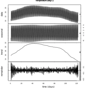
A useful approach [6] is to decompose the given time se-ries data into other three components, trend, season and remainder, as illustrated in the Figure 1.

Temperature (deg C) 10 15 20 25 da ta −6 −2 0 2 4 6 se as on al 14 16 18 20 22 tre nd −0 .3 −0 .1 0. 1 0 20 40 60 80 100 120 re m ai nd er time (days)

Figure 1: Time series decomposition of temperature readings of 120 days.

The trend component can be described by a monotoni-cally increasing or decreasing function (in most cases a linear function) that can be approximated using common regres-sion techniques.

The season component captures recurring patterns that are composed of at least one or more frequencies, e.g. daily, weekly, monthly or yearly patterns. These frequencies can be identified by using a Fast Fourier Transformation (FFT) or by auto-correlation techniques.

The remainder component is an unpredictable overlay of various frequencies with different amplitudes changing 3

http://en.wikipedia.org/wiki/Logistic_regression 4

http://en.wikipedia.org/wiki/Naive_Bayes_ classifier

quickly due to random influences on the time series. The remainder can be reduced by applying smoothing techniques like weighted moving averages (WMA), by using lower sam-pling frequency, or by a low-pass filter that eliminates high frequencies.

3. APPROACH

In this section we present an overview of our proactive adaptation framework, following the self-adaptive reference model K [19]. Our approach implements the MAPE-K structure by:

− Monitoring internal and external context variables. − Introducing predictive analytics to the Analyze

com-ponent.

− Integrating the prediction and reasoning about it in the Planning module.

− Executing the new target reconfiguration using a mod-els@runtime approach [23] to manage actual and po-tential architectural models.

− Exchanging information between these modules through the Knowledge component.

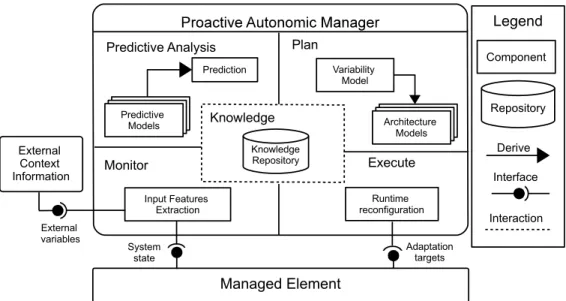
Our architecture is organized in layers as shown in Fig-ure 2. It consists of two detachable subsystems, which are causally connected to each other: the Managed Element and the Proactive Autonomic Manager. Our main contribution is the introduction of the predictive analysis module into the autonomic manager element.

3.1 Monitor Module

Principles.

The monitor module is in charge of keeping continuous record of internal context information. It reads system state variables that hold information about the op-erating environment (e.g. transmission rate, battery level). Regarding external context, the monitoring module also ob-serve external information relevant to the system (e.g. en-vironmental conditions).

Application to fire monitoring.

In order to obtain real data about external context information, we used several existing sources of fire detection data to feed our sensor net-work. Figure 3 shows all fire detections in the year 2010 for the geographic area covering the continental USA including a 50 km buffer around the periphery. The detections were obtained using the Moderate Resolution Imaging Spectro-radiometer (MODIS) and processed as a cooperative effort between the USDA Forest Service Remote Sensing Applica-tions Center, NASA-Goddard Space Flight Center and the University of Maryland. We downloaded these datasets from the USDA website5

.

We have then collected hourly weather readings from sta-tions near spots of fire detecsta-tions. We chose the Integrated Surface Hourly (ISH) datasets6

provided by National Cli-matic Data Center (NCDC). Combining both data sources, we connected individual fires to weather conditions in space and time. Obviously, the fires detected by MODIS are not uniformly distributed throughout the US. Therefore, we have chosen to focus on a geographical area that contains a large amount of fires, namely the state of Mississippi (see Figure 4 5

http://activefiremaps.fs.fed.us/gisdata.php 6

http://www.ncdc.noaa.gov/oa/climate/ surfaceinventories.html

(5)

Knowledge Repository Runtime reconfiguration External Context Information Managed Element System state Adaptation targets Predictive Analysis Knowledge Plan Execute Input Features Extraction Monitor Predictive Models Architecture Models Variability Model Prediction External variables Legend Component Repository Derive Interface Interaction

Figure 2: The proactive adaptation approach.

c o n fi d e n c e

Figure 3: MODIS fire detections in 2010. Over 130,000 fires detected.

and 5) and selected only fires that are within a 50 km radius from an ISH station (see Figure 6).

3.2 Predictive Analysis Module

Principles.

The predictive analysis module receives input from the current state of the system as well as from external context information through the monitor module. We use predictive models and historical information to build the context and model environmental variability. We then feed the reasoning engine with this predictions to improve the decision making process.

Application to fire monitoring.

In the forest monitoring use case we use prediction models to predict the risk of fire in the future. This prediction is taken into account by the planning module to take reconfiguration decisions on the running system.

Area chosen for evaluation

Figure 4: ISH Stations active in 2010 that provided hourly temperature readings. Together 2607 US sta-tions, colors represent states.

To choose good prediction models, we have implemented the prediction of fire risk with the KNIME7

tool, using the Predictive Markup Modeling Language (PMML) [14], which is a standard proposed by the Data Mining Group. In our use case, given a time series of hourly temperature read-ings, we want to predict the fire potential value for the next N hours. This is a classification problem with 13 input at-tributes: the current and the last 9 hours of temperature readings, and average temperature from the past day, week and month. We have selected 8 classification models, as pre-sented in Table 1. These classifiers produce a prediction for the level of temperature: High , Medium and Low. This set of classifiers represents a large panel of existing training-based techniques for automated classification of items into categories.

In order to compare the aforementioned classification mod-els, we needed training and testing data, as well as a scoring method.

7

(6)

Figure 5: Fires in Mississippi detected by MODIS in 2010. Colors represent the nearest ISH station that would detect the fire. (20 ISH stations)

For the training set we used the MERIDIAN NAS temper-ature readings and for the testing set the tempertemper-atures from NACHES/HARDY (AWOS) station. The geographical dis-tance between these two stations is approximately 276 km, which gives us confidence that the results are unbiased. An-other reason for choosing these stations is that there are enough fire detections close to them (for both, approx. 550 fires within the radius of 50 km, see Figure 6), which allows us to later simulate and evaluate the actual running systems. However, these classifiers do not care about fire detections, but rather predict the fire potential based on historical tem-peratures.

We run the train-test evaluation loop 43 times for each classifier while changing the number of hours in future for the fire potential prediction (t + 1, t + 2, . . . , t + 24[1d], t +

Figure 6: Number of fires within 50 km radius from an ISH station. Together 12330 fire detections.

Table 1: Prediction models (classifiers) evaluated. Classifier Training Settings

Multi-Layer Perceptronπ

(0..1) normalization, 3 layers, max. 30 neurons/layer, 300 iter-ations

Fuzzy Rules linear sampling (3000 samples), min/max fuzzy norm

Probabilistic Neural Net

Z-Score norm., Theta -0.1/+0.9 Logistic Regressionπ

– SVMπ

Polynomial kernel, power=0.5 Naive Bayesπ

– Random Forest 100 trees

Functional Trees 30 boosting iterations π

available as a PMML-based model

48[2d], . . . , t + 480[20d])). Each iteration yields several ac-curacy measures (scores). As commonly accepted in the machine-learning community, we used the F1-measure to compare our classifiers (F1 is a harmonic mean of Precision and Recall). By the end of the evaluation, each classifier is characterized by a series of F1-measures depicted in the Figure 7.

+1 +2 +3 +4 +5 +6 +7 +8 +9 +10 +11 +12 +13 +14 +15 +16 +17 +18 +19 +20 +21 +22 +23 +24 +48 +72 +96 +120 +144 +168

Predicted Future [Hours]

0.66

0.68

0.70

0.72

0.74

0.76

0.78

0.80

0.82

0.84

0.86

0.88

0.90

0.92

0.94

0.96

F1

-m

ea

su

re

(hi

gh

er

is

be

tte

r)

Multi Layer Perceptron

Probabilistic Neural Network

Fuzzy Rule Model

Support Verctor Machine

Logistic Regression

Naive Bayes

Random Forest

Functional Trees

Training:MERIDIAN NAS, Testing: NATCHEZ/HARDY,

Distance between locations:276 km

Figure 7: Comparing different classification models using data from distant stations.

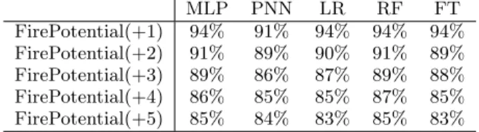
We clearly see that most of our classification models achieve a pretty high prediction performance. For instance, predict-ing 5 hours in the future can be achieved with F1 = 85% accuracy, as depicted in Table 2. Moreover, even 20 days in future can be predicted with more than 75% F1. In our experiment, we only used predictions from 1, 2, . . . , 7 hours in future.

We finally selected the Multi Layer Perceptron (MLP) model because it gives almost the highest accuracy. In con-trast to the best performing Random Forest (RF) model, MLP is available as a PMML model. Training MLP re-quires more time than RF. However it must be done only once, and running predictions using MLP is faster than RF.

(7)

A trained MLP model consists of 63 neurons organized in 3 layers, with a network of 13 inputs and 3 outputs. The rest of the text therefore assumes the use of MLP as a classifier.

Table 2: F1-measures of 5 best performing classifi-cation models predicting fire potential outcome for 1 to 5 hours in future. MLP PNN LR RF FT FirePotential(+1) 94% 91% 94% 94% 94% FirePotential(+2) 91% 89% 90% 91% 89% FirePotential(+3) 89% 86% 87% 89% 88% FirePotential(+4) 86% 85% 85% 87% 85% FirePotential(+5) 85% 84% 83% 85% 83%

3.3 Plan Module

Principles.

Most of the current self-adaptive approaches use decision techniques such as Event Condition Actions (ECA) [27]. An ECA technique that uses instantaneous values of context variables is purely reactive. In our case, we adopt an ECA technique with events based on predic-tions. These events carry aggregate information of previous historic data plus the foresight into the prediction horizon. Conditions remain conceptually the same: they can be as simple as a threshold. Finally, an action is generated in reply to a condition.

Application to fire monitoring.

To illustrate our proac-tive adaptation in our fire potential scenario, let us assume the following constraints in the system:

− time for redeploying a reconfiguration is 1 time unit; − there are three levels of sensing rates: high (every

hour), medium (every 8 hours), and low (every 24 hours). Using the temperature prediction, we have implemented the following ECA rule:

Event: An increase or decrease in temper-ature.

Condition: If the temperature crosses the threshold in ascending or descend-ing manner.

Action: The system will increase or decrease the sensing rate accordingly.

Let us consider the following scenario that lasts 3 time units, where we represent the system state with a (sensing-rate, temperature) tuple as follows:

− 0. (medium sensing rate, medium temperature) − 1. (medium sensing rate, high temperature) − 2. (high sensing rate, medium temperature) − 3. (medium sensing rate, medium temperature) Following a reactive approach, the system triggers a re-configuration after 1 time unit, because the previous tem-perature reading was high. However by the time the re-configuration has taken place the temperature has dropped back to medium level, making this reconfiguration useless and consuming extra energy.

Following our predictive approach, the system does not take decisions on instantaneous values of environmental vari-ables, but it considers the trend and the seasonal compo-nents of the historical data, plus the forecast of the variables, thus avoiding this useless reconfiguration.

3.4 Execute Module

The goal of this module is to deploy the new system con-figuration decided by the planning module on the running system. We use Kevoree [11], a models@rutime tool that provides a reflection model of the running system, then al-lows edition of this model and generation of a new target model. This target model can then be redeployed and syn-chronized with the running system.

Kevoree targets distributed systems, ranging from sen-sor networks to cloud systems. It particularly provides dis-tributed synchronization of models@runtime[10]. In the fire monitoring scenario, we mainly target sensor network nodes where reconfigurations have to be disseminated among dis-tributed nodes. Kevoree addresses the reconfiguration of these resource constrained nodes by providing two recon-figuration types: parametric reconrecon-figurations and firmware updates. Parametric reconfigurations are used when the change only involves modification of variable values. Firmware updates are used in all other situations. A firmware update reconfiguration has a higher cost as it involves flashing the firmware of the sensor nodes.

Using Kevoree we are able to disseminate reconfigurations to dynamically update the behavior of the sensor nodes. Particularly to our case study, these reconfigurations con-sist in activating or deactivating, changing the sensing rate or flashing the firmware of the sensor nodes.

3.5 Knowledge Module

In Figure 2, the dotted line between the knowledge el-ement represent interaction. The purpose of the knowl-edge repository is the continuous exchange of information between all the modules.

For the serialization of prediction models we use the Pre-dictive Model Markup Language language (PMML) [14]. As previously mentioned, PMML is an XML-based language that enables the definition and sharing of predictive models and can be easily integrated in KNIME, which allowed us to implement classifier and forecast models. These files can be imported or exported inside a KNIME workflow and are ready for use within the running nodes.

4. VALIDATION

We performed an experimental study on the fire monitor-ing scenario to validate our approach. We defined the exper-imental design of our study using the Goal-Question-Metric method. The GQM method was defined as a mechanism for defining and interpreting a set of operation goals, using measurements [1]. In this experiment, our goal is the follow-ing:

Purpose: Improve

Issue: the global effectiveness Object : the system

Context: self-adaptive sensor networks

To fulfill this goal, we will focus on answering the three following research questions:

1. RQ1: Does a proactive adaptation approach trigger less reconfigurations than a reactive approach under seasonal behavior conditions?

2. RQ2: Does a proactive adaptation approach improve energy consumption compared with a reactive adapta-tion approach?

(8)

3. RQ3: Does a proactive adaptation approach reduce the delay in transmitting fire alert in comparison to a reactive approach?

We then defined our experiment type. V. Basili described two kinds of studies: in-vivo and in-vitro [1]. Later, two more categories were added: in-virtuo, in-silico [15]. In our case, we chose to carry in-silico experiments, where subjects and real world are described as computer models. The en-vironment is composed entirely of computer models, with which human interaction is reduced to a minimum. This of-fers major advantages regarding cost and feasibility of repli-cating a real-world configuration.

To answer these research questions, we set up an exper-iment where we simulated 10 baselines and 28 predictive systems. Our assumptions common to all of these systems are as follows:

− The shortest time unit is one hour.

− Each system operates in a certain interval that is either constant or varies over time, depending on the type of a system. If the interval changes, we consider it as an adaptation. For each system, we compute the number Aas the number of adaptations in the year.

− In every iteration, the system reads its sensors and sends the data to the data collector. For each system, we compute the number T as the number of transmis-sions in a year.

− When a fire is detected by a system, we compute the number of hours that the fire should have been re-ported to the base station. We call this measure “Late Fire Hours” λi. We compare all systems based on: L= Σh

i=1λi, where h is the number of all hours in the year.

− Using the metrics above, we define power consumption metrics as P = 0.1 ∗ T + 0.5 ∗ A.

− We also compute relative versions of the metrics AR , TR

, PR

and LR

that are relative to the reactive sys-tem.

Reactive system.

This is our first baseline system that adapts its transmission rate based on the current temperature.

Simple system.

This is also a baseline system with a con-stant transmission rate. We simulated 9 variants with dif-ferent transmission rates: 1, 2, 3, 4, 5, 6, 7, 8, 12.

Predictive system.

This system operates similarly to the reactive system. However, before each adaptation it uses a classifier to predict fire potential at time t + F (t is current time, F is the number of hours in future). The adaptation is cancel whenever

F ireP otential(t − 1) = F ireP otential(t + F ) There are 4 variants of this system:

− The default variant uses prediction before any adapta-tion.

− The variant denoted as “D” (slowing down without pre-diction) runs the prediction only if changing from lower transmission rate to higher transmission rate.

− The variant denoted as “U” (speeding up without pre-diction) runs the prediction only if changing from higher transmission rate to lower transmission rate.

− The variant denoted as “i” (interval check) runs predic-tion for all hours in the interval t+1, t+2, . . . , t+F , so that there is a higher chance to cancel the adaptation. We executed our simulation of the 38 systems on all fires detected close to the NACHES/HARDY (AWOS) station and collected the results, which are depicted in Figures 8 Figure 9 and Figure 10. Each figure shows a comparison of the systems using different metrics.

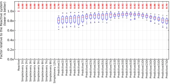
RQ1: Evaluating reconfigurations.

Figures 8 relates to RQ1 and depicts the number of recon-figurations for each self adaptive systems. From this result, we can observe that all 28 systems based on proactive adap-tations are achieving a smaller number of reconfigurations than a reactive system. We are able to save up to 20 % of the number of reconfigurations of the system with the Predic-tive(1) system. These results highlight that using predictive information can help to reduce the number of reconfigura-tions of a system.

RQ2: Evaluating System lifetime.

Figure 9 relates to RQ2 and depicts the total power con-sumption for each type of a systems. We use this metric to quantify the lifetime of the system as the lifetime is directly correlated to total power consumption. For this metric, all the predictive systems reduced the power consumption with respect to Reactive system. The lowest power consump-tion has been measured in the Predictive(*)D and Predic-tive(*)Di group. In other words, when choosing an adequate adaptation strategy, these results show that using prediction information allows for an increase in system lifetime.

RQ3: Evaluating late fire report.

Figures 10 relates to RQ3 and presents the delay intro-duced in reporting fire alerts for each self adaptive systems. From these results, we can observe that most of the pre-dictive techniques show fire detection delays similar to the reactive approach technique. This result is valuable since proactive techniques such as Predictive(3)U were able to decrease the number of system reconfigurations, while pro-viding a smaller delay for detecting fire. On these results, we can also observe that the Predictive(*)Di techniques are exhibiting larger delays than the other approaches. This is due to the fact that this proactive adaptation strategy tends to slow down the adaptation process.

We want to emphasize that the three parameters eval-uated in these three research questions are contradictory. Indeed, minimizing power consumption and minimizing the delay for detecting fire are contradictory objectives since one objective requires minimal sensing rate, where the other ob-jective requires maximum sensing rate. In our result, the Predictive(3)U has performed better than the Reactive ap-proach in all these experiments.

This case study demonstrates how a proactive approach can be more efficient over a long period of time than a re-active approach. This conclusion agrees with S.W.Cheng et al. [8] in that reactive adaptation has two deficient prop-erties: (1) information used for decision making does not extend into the future, and (2) the planning horizon of the strategy is short and does not consider the effect of current decisions on future utility [8].

(9)

Reactive

Simple(every 1h) Simple(every 2h) Simple(every 3h) Simple(every 4h) Simple(every 5h) Simple(every 6h) Simple(every 7h) Simple(every 8h) Simple(every 12h) Predictive(1) Predictive(2) Predictive(3) Predictive(4) Predictive(5) Predictive(6) Predictive(7) Predictive(1)U Predictive(2)U Predictive(3)U Predictive(4)U Predictive(5)U Predictive(6)U Predictive(7)U Predictive(1)D Predictive(2)D Predictive(3)D Predictive(4)D Predictive(5)D Predictive(6)D Predictive(7)D Predictive(1)Di Predictive(2)Di Predictive(3)Di Predictive(4)Di Predictive(5)Di Predictive(6)Di Predictive(7)Di

0.0x

0.2x

0.4x

0.6x

0.8x

1.0x

Factor relative to the Reactive system

(lower is better)

1.00 0.00 0.00 0.00 0.00 0.00 0.00 0.00 0.00 0.00 0.79 0.82 0.83 0.83 0.83 0.83 0.85 0.87 0.89 0.89 0.89 0.90 0.89 0.92 0.91 0.93 0.93 0.93 0.93 0.92 0.93 0.91 0.89 0.88 0.86 0.83 0.81 0.79

Figure 8: Number of needed reconfigurations relative to the reactive system

Reactive

0.0x

0.2x

0.4x

0.6x

0.8x

1.0x

Factor relative to the Reactive system

(lower is better)

1.00 1.22 0.61 0.41 0.31 0.24 0.20 0.17 0.15 0.10 0.93 0.94 0.94 0.94 0.95 0.94 0.95 0.98 0.98 0.98 0.97 0.98 0.98 0.98 0.94 0.96 0.97 0.96 0.97 0.96 0.96 0.94 0.93 0.92 0.89 0.88 0.85 0.84

Figure 9: Total power consumption relative to the reactive system.

5. RELATED WORK

Since the 70s, software maintenance has been studied from different perspectives: corrective, adaptive (reactive) and perfective [29]. In this paper we are focusing in the tem-poral characteristic of the adaptation. Research efforts in prediction include a large variety of domains such as: online failure prediction[28, 32], resource and demand prediction [2, 16], and user behavior prediction[30], among others.

A key reference work with which we share conceptual sim-ilarities, is the one done by V. Poladyan [25] and later on complemented by S.W.Cheng et. al. in [8]. However, as it was recognized by co-author D.Garlan in [13], their approach has some limitations such as: a fixed set of reconfiguration strategies, limitation to repair triggered by constraint vio-lations, which is a corrective adaptation category. Our ap-proach differ from this work by using a strategy focused on aggregate utility rather than instantaneous utility. In the same keynote D.Garlan pointed out that in many cases it

may be better to do things before the problem occurs, by using proactivity.

Epifani et. al. argue in [9] that it is possible to detect or predict if a desired property is, or will be, violated by the running implementation. They focus on properties such as reliability and performance, using Discrete Time Markov Chains (DTMCs) and Queuing Networks (QNs). In our case we evaluated eight different non-linear prediction models. Yet we share a clear separation between detection and pre-diction (failure detection and failure prepre-diction in their case, fire detection and fire prediction in ours).

In the context of online failure predictions, failures are the events that trigger adaptation [28, 32]. These events correspond to failures such application-level exceptions and infrastructure-level failures, changes in contextual settings (such as execution environment and usage context), changes in available services and their characteristics, and modifi-cations of business-level properties (e.g. key performance

(10)

Reactive

0x

2x

4x

6x

8x

10x

12x

14x

16x

Factor relative to the Reactive system

(lower is better)

1.00 0.00 0.72 2.76 _12.38 _15.34 9.24 _24.28 _43.93 _43.89 2.34 1.72 1.35 1.40 1.40 1.37 1.51 1.02 1.00 0.95 0.99 0.98 0.98 0.98 2.33 1.70 1.39 1.38 1.37 1.39 1.53 2.33 2.64 2.68 2.74 2.81 3.03 3.46

Figure 10: Number of hours when a fire detected by the node was waiting for transmission to the data collector. The number is relative to reactive system.

indicators). Adaptation requests (also known as adaptation requirements or specifications) specify how the underlying application should be modified upon the occurrence of the associated event or situation. Reactiveness to this kind of failures is necessary yet often insufficient for some domains. Pro-activeness decreases the aftereffects of changes, or im-proves control of change propagation (e.g. in environment monitoring, safety-critical systems) [27, 17].

Resource prediction as conceived by [2, 16, 25] refers to estimating the available level of a resource in the near future, (e.g., in the next 10 seconds). Resource demand prediction refers to the prediction of how much resource an applica-tion will consume in a particular setting. In our work we are interested in predicting resource needs and availability but in predicting changes in internal and external context information that may trigger adaptations.

Some criticism about predicting human behavior is that a person can change his mind from one day to another and does not necessarily take the same decision if is put in the same conditions. We differ from [30], as we are focusing on predicting environment behavior based on historical data, where is it easier to identify trend and seasonal components. Typical self adaptive systems SAS based on model@runtime are causally connected self-representations of the associated system that emphasizes the structure, behavior, or goals of the system from a problem space perspective [22]. However they reason on current values of structure properties, be-havior, or goals. This kind of approach does not take into consideration previous history data, although it may explain occurrences of rapidly changing conditions.

Hielscher et al. [17] proposed PROSA, an online testing-based proactive self-adaptation. Firstly, they aim at predict-ing new failures from past monitorpredict-ing data, but their goal is to detect whether one specific failure that has been un-covered in on aService-Based Applications (SBA) could also occur in other SBA instances. Secondly, in [17] the authors reject past monitoring data after a dynamic adaptation of the system. In doing this the system may fall into cyclical adaptations without detecting it.

6. CONCLUSION AND FUTURE WORK

The proposed proactive approach is not restricted to the case study we have chosen to evaluate but can be applied to a wide range of applications, namely applications with well defined input parameters that can be represented as mathe-matical functions (e.g. forecasts of bandwidth demand and supply), or critical systems with seasonal behavior (e.g. min-imizing power consumption when conditions are safe).

In this paper we evaluated the benefits of anticipating a problem. The validation of our approach on the fire moni-toring case study have shown interesting results that confirm the idea that pro-active adaptation based on predictive an-alytics is a promising research direction.

Indeed, the benefits of predictive analysis combined with proactive adaptation techniques out weights its overhead when compared with a purely reactive approach. However, our approach can be improved in several ways. One of those ways is to draw more detailed energy consumption models. of wireless sensor networks. In the near future we would like to explore the risk associated with the late reporting and its trade-offs between those risks and the power usage.

We plan to investigate a distributed reasoning engine in place of its current centralized version.

Another aspect worth considering is back-to-back adapta-tions, i.e when adapting a component in a system triggers chain reactions that causes further adaptations in other com-ponents. Complex problems may result from these chain reactions like infinite triggering of new adaptations or in-consistent configurations in different components. In future work we plan to consider these scenarios.

7. ACKNOWLEDGMENTS

The research presented in this paper is supported by the European Union within the FP7 Marie Curie Initial Training Network ”RELATE” under grant agreement number 264840.

(11)

8. REFERENCES

[1] V. R. Basili. The role of experimentation in software engineering: past, current, and future. In Proc. of the 18th international conference on Software engineering, pages 442–449. IEEE Computer Society, 1996. [2] S. Becker, H. Koziolek, and R. Reussner. The Palladio

component model for model-driven performance prediction. Journal of Systems and Software, 82(1):3–22, 2009.

[3] M. Berthold, C. Borgelt, and F. H¨oppner. Guide to intelligent data analysis, volume 42. Springer, 2010. [4] M. R. Berthold. Mixed fuzzy rule formation.

International journal of approximate reasoning, 32(2):67–84, 2003.

[5] M. R. Berthold and J. Diamond. Constructive training of probabilistic neural networks. Neurocomputing, 19(1-3):167–183, 1998.

[6] G. E. Box, G. M. Jenkins, and G. C. Reinsel. Time series analysis: forecasting and control. Wiley, 2013. [7] L. Breiman. Random forests. Machine learning,

45(1):5–32, 2001.

[8] S.-W. Cheng, V. V. Poladian, D. Garlan, and B. Schmerl. Improving architecture-based self-adaptation through resource prediction. In Software Engineering for Self-Adaptive Systems, pages 71–88. Springer, 2009.

[9] I. Epifani, C. Ghezzi, R. Mirandola, and G. Tamburrelli. Model evolution by run-time parameter adaptation. In IEEE 31st International Conference on Software Engineering, pages 111–121. IEEE, 2009.

[10] F. Fouquet, E. Daubert, N. Plouzeau, O. Barais, J. Bourcier, and J.-M. J´ez´equel. Dissemination of reconfiguration policies on mesh networks. In Distributed Applications and Interoperable Systems, pages 16–30. Springer Berlin Heidelberg, 2012. [11] F. Fouquet, B. Morin, F. Fleurey, O. Barais,

N. Plouzeau, and J.-M. Jezequel. A dynamic

component model for cyber physical systems. In Proc. of the 15th ACM SIGSOFT symposium on Component Based Software Eng., pages 135–144. ACM, 2012. [12] J. Gama. Functional trees. Machine Learning,

55(3):219–250, 2004.

[13] D. Garlan. A 10-year perspective on software engineering self-adaptive systems (keynote). In Proc. of the 8th Int. Symposium on Software Engineering for Adaptive and Self-Managing Systems, pages 2–2. IEEE Press, 2013.

[14] A. Guazzelli, M. Zeller, W. Lin, and G. Williams. PMML : An Open Standard for Sharing Models. The R Journal, pages 60–65, 2009.

[15] M. O. B. Guilherme Horta Travassos. Contributions of in virtuo and in silico experiments for the future of empirical studies in software engineering. In Proc. of the ESEIW 2003 Workshop on Empirical Studies in Software Engineering. IEEE Computer Society, 2004. [16] N. R. Herbst, N. Huber, S. Kounev, and E. Amrehn. Self-adaptive workload classification and forecasting

for proactive resource provisioning. In Proc. of the ACM/SPEC International Conference on Performance Engineering (ICPE), pages 187–198. ACM, 2013. [17] J. Hielscher, R. Kazhamiakin, A. Metzger, and

M. Pistore. A framework for proactive self-adaptation of service-based applications based on online testing. In Towards a Service-Based Internet, pages 122–133. Springer, 2008.

[18] S. S. Keerthi, S. K. Shevade, C. Bhattacharyya, and K. R. K. Murthy. Improvements to platt’s smo algorithm for svm classifier design. Neural Computation, 13(3):637–649, 2001.

[19] J. O. Kephart and D. M. Chess. The vision of autonomic computing. Computer, 36(1):41–50, 2003. [20] N. Landwehr, M. Hall, and E. Frank. Logistic model

trees. Machine Learning, 59(1-2):161–205, 2005. [21] T. Mitsa. Temporal data mining. CRC Press, 2010. [22] B. Morin, O. Barais, J.-M. J´ez´equel, F. Fleurey, and

A. Solberg. Models@ run. time to support dynamic adaptation. Computer, 42(10):44–51, 2009.

[23] B. Morin, O. Barais, G. Nain, and J.-M. Jezequel. Taming dynamically adaptive systems using models and aspects. In Proc. of the 31st International Conference on Software Engineering, pages 122–132. IEEE Computer Society, 2009.

[24] J. C. Platt. 12 fast training of support vector

machines using sequential minimal optimization. 1999. [25] V. Poladyan. Tailoring Configuration to User’s Tasks

under Uncertainty. PhD thesis, Carnegie Mellon University, 2008.

[26] M. Riedmiller and H. Braun. A direct adaptive method for faster backpropagation learning: The rprop algorithm. In IEEE International Conference on Neural Networks, pages 586–591. IEEE, 1993.

[27] M. Salehie and L. Tahvildari. Self-adaptive software: Landscape and Research Challenges. ACM

Transactions on Autonomous and Adaptive Systems, 4(2):1–42, May 2009.

[28] F. Salfner, M. Lenk, and M. Malek. A survey of online failure prediction methods. ACM Computing Surveys, 42(3):1–42, Mar. 2010.

[29] E. B. Swanson. The dimensions of maintenance. In Proc. of the 2nd international conference on Software engineering, pages 492–497. IEEE Computer Society Press, 1976.

[30] V. S. Tseng and K. W. Lin. Efficient mining and prediction of user behavior patterns in mobile web systems. Information and software technology, 48(6):357–369, 2006.

[31] J. Wu and S. Coggeshall. Foundations of Predictive Analytics. Chapman & Hall/CRC data mining and knowledge discovery series. CRC PressINC, 2012. [32] L. Yu, Z. Zheng, Z. Lan, and S. Coghlan. Practical

online failure prediction for blue gene/p: Period-based vs event-driven. In Dependable Systems and Networks Workshops (DSN-W), 2011 IEEE/IFIP 41st

International Conference on, pages 259–264. IEEE, 2011.