A constitutive model for Ti6Al4V considering the state of stress and strain rate effects

Science Arts & Métiers (SAM)

is an open access repository that collects the work of Arts et Métiers Institute of Technology researchers and makes it freely available over the web where possible.

This is an author-deposited version published in: https://sam.ensam.eu

Handle ID: .http://hdl.handle.net/10985/18139

To cite this version :

Wenyu CHENG, José OUTEIRO, Jean-Philippe COSTES, Rachid M'SAOUBI, Habib KARAOUNI, Viktor ASTAKHOV - A constitutive model for Ti6Al4V considering the state of stress and strain rate effects - Mechanics of Materials - Vol. 137, p.103103 (17 p.) - 2019

A constitutive model for Ti6Al4V considering the state of stress

and strain rate effects

Wenyu Cheng

_{, Jose Outeiro}

, Jean-Philippe Costes

, Rachid M’Saoubi

,

Habib Karaouni

_{, Viktor Astakhov}

a

Arts et Metiers ParisTech, LaBoMaP, Rue Porte de Paris, 71250 Cluny, France b

R&D Material and Technology Development Seco Tools AB, SE-73782 Fagersta, Sweden c

Safran Tech, Research and Technology Center, 78772 Magny-Les-Hameaux, France d

General Motors Business Unit of PSMi, 1792, Elk Ln, Okemos, MI 48864, USA Abstract

The predictability of manufacturing process simulation is highly dependent on the accuracy of the constitutive model to describe the mechanical behavior of the work material. The model should consider the most relevant parameters affecting this behavior. In this study, a constitutive model for Ti6Al4V titanium alloy is proposed that considers both material plasticity and damage. It includes the effects of strain hardening, strain-rate and the state of stress to represent the mechanical behavior of Ti6Al4V titanium alloy in metal cutting simulation. To generate states of stress and strain rates representative of this process, mechanical tests were performed using a specific experimental setup. This included a specimen geometry designed to generate different states of stress, as well as a digital image correlation technique to obtain the strains during the mechanical tests. For the determination of the coefficients of the constitutive model, the yield stress and fracture locus obtained from these tests were used in an optimization-based procedure. To verify the accuracy of the proposed constitutive model to represent the mechanical behavior of the Ti6Al4V alloy under different states of stress, force-displacement curves obtained using this model and the Johnson-Cook model are compared with the curves obtained experimentally.

Keywords: Constitutive behavior; Mechanical testing; Fracture mechanisms; Manufacturing Processes.

1. Introduction

Ti6Al4V titanium alloy plays a significant role in a broad range of applications, such as those related to aerospace, automotive and biomedical industries. This alloy has useful application properties, i.e., high strength/weight ratio, acceptable mechanical strength at high temperatures, high resistance to creep and corrosion [1]. This alloy is also difficult to cut due to its high strength, low thermal conductivity and high chemical reactivity [2]. Therefore, tool wear is accelerated and the resulting surface integrity can be very poor [2]. A proper choice of the cutting tool and corresponding cutting parameters can solve these issues. An effective and economical approach to accomplish this selection is to perform numerical simulations. It is a cost-effective approach when compared to the traditional experimental approach. However, the precision of the simulated results is strongly affected by the material constitutive model that represents the mechanical properties of the work material [3,4].

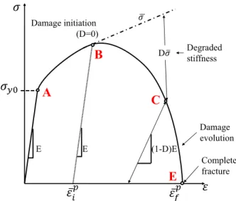
Fig. 1 represents schematically a typical stress-strain curve of a mechanical test, presenting the

elastic and plastic material response until fracture. The solid line represents the typical (experimental) strain curve, while the dashed dot line is a hypothetical undamaged stress-strain curve. As shown, the two lines begin to separate at point B, which denotes the damage initiation. After this point, the yield strength and elastic modulus degrade as the strain increases. The difference between these two lines is estimated by the damage parameter D. The occurrence of complete fracture is at point E when D equals 1.

To describe this mechanical behavior starting from elastic-plastic deformation to complete fracture, two parts should be included in the constitutive model: plasticity and damage. For the plasticity part of the constitutive model, the Johnson-Cook (J-C) model is extensively used in commercial finite element analysis (FEA) software [6]. This model can be used in numerous situations, including: high velocity impact, metal forming, metal forging and machining. However, the model coefficients are very sensitive to any changes in the metallurgical conditions of the work material. For such reason, different coefficients can be found in the literature for the J-C model of Ti6Al4V alloy [7-9]. Several metal cutting researchers have modified this model to improve its ability to reproduce the mechanical behavior. A so-called strain-softening term was integrated into the J-C model by Calamaz et al. [10], to better predict the segmented chip with small uncut chip thickness and low cutting speed in orthogonal cutting simulation of Ti6Al4V alloy. Sima and Ozel [11] did a minor modification of the Calamaz et al. [10] model to further control the thermal softening effect. However, some model coefficients were determined by fitting between the measured and the predicted results from orthogonal cutting tests, without performing any material characterization tests. Moreover, the applicability of both modified J-C models to other manufacturing processes still needs to be verified. Santos et al. [12] also proposed a modified J-C model that includes what they called flow softening, which fits the stress-strain curves of AA1050 aluminum alloy obtained from tests at high strain rates better, when compared to the traditional J-C model.

The plasticity models described above are designed as phenomenological since the material behavior is described by empirically fitted functions, which contain several macroscopic deformation variables, such as temperature, plastic strain and plastic strain rate. Other types of plasticity model are those mentioned by Melkote et al. [4] as physical-based models, since they integrate microstructural aspects (i.e., grain-size, dislocation density, etc.) in the material mechanical behavior. One case is the Mechanical Threshold Stress (MTS) model [13], involving both the thermal and athermal stresses related to the dislocation density and grain size. Melkote et al. [14] extended the MTS model to simulate chip formation of pure titanium. The effects of dynamic recovery, dislocation drag and dynamic recrystallization were considered in their model. Although these models intrinsically describe the microstructure evolution and mechanical behavior of the work material, their complexity regarding the large number of coefficients to be determined through several types of experimental tests limits their application.

proposed by Calamaz et al. [10], and then applied it in orthogonal cutting simulation of Ti6Al4V alloy under cryogenic cooling conditions.

These works do not account for the damage part of the constitutive model, which is fundamental for those applications where fracture occurs, as is the case for the metal cutting process [16]. Moreover, none of these works considers the state of stress effect on plasticity and damage. As far as this effect is concerned, Rice and Tracey [17] described the ductile fracture process as the growth and coalescence of microscopic voids under the superposition of hydrostatic stresses. Then, a fracture locus was introduced based on the ratio between the hydrostatic and the equivalent stresses, often referred to as stress triaxiality. This model has been widely adopted by other researchers. For example, Johnson and Cook [6] proposed a damage model accounting for several effects on damage initiation: stress triaxiality, strain rate and temperature. Bai and Wierzbicki [18,19] also considered the Lode angle effect on the fracture locus apart from the stress triaxiality effect. They proposed a constitutive model considering the state of stress, described by both stress triaxiality and Lode angle. They have shown that both parameters affect, not only the fracture, but also the plasticity behavior of AA2024-T351 aluminum alloy. As shown in Fig. 1, damage cannot be represented accurately by considering the fracture locus only. Hence, damage evolution should also be considered. Hillerborg et al. [20] proposed a fracture energy formulation that is often used to describe damage evolution.

Several researchers have used constitutive models integrating the damage part for metal cutting simulation. For instance, Buchkremer et al. [21] extended both the plasticity and the damage models proposed by Bai and Wierzbicki [18,19] by including the temperature and strain-rate effects. They predicted the forces, temperatures, chip formation and flow with high accuracy in simulation of turning AISI 1045 steel. Denguir et al. [22] proposed a constitutive model (plasticity and damage) incorporating, not only the strain-hardening, strain-rate and temperature effects, but also the microstructural and state of stress effects to describe the mechanical behavior of Oxygen Free High Conductivity (OFHC) copper in metal cutting. They showed better surface integrity prediction when the proposed constitutive model was compared with the J-C model. Abushawashi et al. [23] found that the material plastic strain limit in the first deformation zone is controlled by the value of stress triaxiality in orthogonal cutting of AISI 1045 steel. Wang and Liu [24] investigated the stress triaxiality effect on the generation of segmented chips during machining of Ti6Al4V alloy. It was found that its value in the first deformation zone ranges from -0.6 to 0.6. Liu et al. [25] have shown that the chip formation in

orthogonal cutting of AA2024-T351 aluminum alloy is simulated better when damage evolution is considered instead of damage initiation only.

This paper proposes a constitutive model for Ti6Al4V titanium alloy. This model includes the most relevant parameters affecting the mechanical behavior (plasticity and damage) of this alloy in the first deformation zone in metal cutting, such as: strain hardening, strain rate and state of stress. The latter is represented by the stress triaxiality and the Lode angle, normally ignored in the existing constitutive models used in metal cutting simulations. Moreover, this paper also presents a complete methodology to conduct the mechanical tests for accurate determination of the constitutive model coefficients. Mechanical tests are performed using a specially designed experimental setup (including tailored specimen geometries) to generate the wide range of state of stress (i.e. triaxiality and Lode angle) found in various machining operations. An optimization-based procedure was developed to determine the coefficients of the constitutive model, using experimental data from the mechanical tests and finite element simulations of those tests. Finally, the accuracy of proposed model is demonstrated by comparing the force-displacement curves obtained using this model, the J-C model and the experimental results.

2. Proposed constitutive model 2.1 State of stress definition

Because this paper involves the relationship between the mechanical behavior of Ti6Al4V alloy and the state of stress, the notion of state of stress should be clarified. It is represented by the stress triaxiality and Lode angle parameter, as shown in Fig.2. An arbitrary stress tensor [σij]

can be represented by three principal stresses: σ1, σ2, σ3. The stress triaxiality  is defined as

the ratio of the mean stress m to the equivalent von Mises stress 𝜎̅.

1 2 3 m 1 3 3 I         + + = = = (1)

The Lode angle parameter 𝜃̅ proposed by Bai and Wierzbick [18] is used to describe the effect of the Lode angle in this paper. Fig. 2 illustrates the definition of the Lode angle on the

deviatoric plane and the directions of the principal stresses. The Lode angle 𝜃 is defined as follows: 3 3

1

27

arccos

3

2

J









=

_

_





where J3 is the third deviatoric stress invariant. The following equation shows the Lode angle

parameter:

6 1

π

 = −  (3)

where 𝜃̅ is the Lode angle parameter. The range of 𝜃̅ is [-1, 1], as the range of Lode angle 𝜃 is [0, 𝜋/3]. These equations show that the stress triaxiality depends on the first stress invariant I1,

while the Lode angle is a function of the third deviatoric stress invariant J3 and the von Mises

equivalent stress, 𝜎̅.

(a) (b)

Fig. 2: a) The space of principal stresses; b) Lode angle definition on the  plane [18].

2.2 Constitutive model formulation

Two parts are included in the proposed constitutive model: plasticity and damage. The proposed plasticity model is shown in Equation (4), incorporating the strain hardening, strain rate and state of stress effects. The first two terms are based on the Johnson - Cook [6] and Santos et al. [12] models, respectively. Furthermore, the last two terms of Equation (4) are related to the state of stress effect, which are characterized by the stress triaxiality and the Lode angle parameter obtained from the Bai and Wierzbicki [18] model.

(

)

(

)

(

)

strain hardening effect strain-rate effect stress triaxiality effect Lode angle effect

(

)

In the previous equations: i) the coefficients A, m and n are used in the strain hardening term; ii) the coefficients 𝐵 , 𝐶 and 𝐸 are used in the strain rate term; iii) the coefficient 𝑐_η is used in the stress triaxiality term; iv) the coefficients 𝑐_θt, 𝑐_θc, 𝑐_𝜃𝑠 and a are used in the Lode angle term; v) 𝜂0 is the reference stress triaxiality and 𝜀̇0 is the reference strain rate; vi) γ describes the

difference between Tresca and von-Mises equivalent stresses on the deviatoric stress plane, as represented in Equation (5); and vii) the coefficients 𝑐_θt, 𝑐_θc, 𝑐_θs are interdependent and at least one of them equals 1. Considering the compression test of cylindrical specimen at quasi-static conditions as a reference, 𝜂0 equals -1/3, 𝜀̇0 equals 0.05 s-1 and 𝑐θc equals 1.

The temperature effect on the work material behavior is not considered in this plasticity model for two main reasons. First, the temperature effect has been included in the high strain rate mechanical tests since the work of plastic deformation is converted into heat. Second, the temperature in the first deformation zone of the workpiece rarely exceeds 200°_{C in the metal}

cutting process, because of the heat advection (i.e. mass transportation) through the chip movement [26,27]. Indeed, a very significant amount of the heat generated due to plastic deformation in the first deformation zone will be transported by the chip due to advection, while a smaller portion of this generated heat will flow into the workpiece by conduction. The ratio between these two parts can be determined by the Péclet number [26], as shown by Equation

(7), Heat of advection Heat of conduction VL Pe w = = (7)

When the Péclet number is applied to metal cutting, V represents the chip velocity relative to the tool rake face (m/s), L represents the uncut chip thickness (mm) and 𝑤 represents the thermal diffusivity (m2_{/s). For example, in orthogonal cutting of Ti6Al4V alloy using typical}

cutting conditions (cutting speed Vc = 0.917 m/s (55 m/min) and L = 0.15 mm) the chip

compression ratio ζ is equal to 1.5, and considering the thermal diffusivity 𝑤 of Ti6Al4V alloy as equal to 7.15 x 10-6 m2/s, the Péclet number is equal to 12. Therefore, 92% of the heat produced in the first deformation zone flows into the chip due to the plastic deformation, while only 8% of this heat flows into the workpiece.

The damage model includes damage initiation and damage evolution, as shown from Equation

(8) to (10), based on Bai and Wierzbicki [18] and Abushawashi [28] models. Equation (8)

represents the damage initiation, while Equations (9) and (10) represent the damage evolution. Fracture surface depends on both the stress triaxiality and Lode angle parameter. The work material strength decreases as the strain increases after damage initiation, and the fracture energy is used to estimate this material stiffness degradation.

(

)

(

)



(

)

( )

_{( )}

_

_

In these equations, D1-D7, n, and Gf are the material coefficients, 𝜆 controls the material

degradation rate and Gf is the material fracture energy density; 𝜀̅_ip is the plastic strain at damage

initiation; 𝜀̅_fp is the plastic strain when all the stiffness and the fracture energy of the material have been lost and dissipated, respectively; 𝜎̃ is the hypothetical undamaged stress evaluated by Equation (4); 𝑙 is the characteristic length of the finite element; 𝜇̅ = 0 relates to the equivalent plastic displacement before damage initiates; and 𝜇̅f is the equivalent plastic

As shown in Equation (10), the characteristic length is introduced to describe the fracture energy. Therefore, the energy dissipated in the damage evolution is defined as per unit area, rather than per unit volume. In this case, a displacement response instead of the stress-strain response is used to describe the material softening after damage initiation.

3. Mechanical tests

3.1 Specimen’s material and geometry

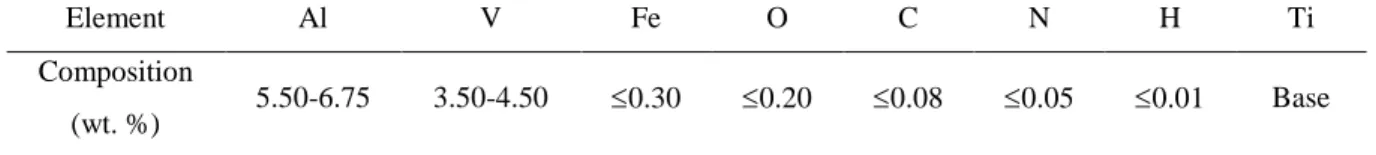
The chemical composition of Ti6Al4V alloy used in this research work is presented in Table 1. This material has a two-phase structure (𝛼+𝛽), and the good balance between 𝛼 and 𝛽 phases makes it achieve a high strength level without losing ductility [1].

Table 1: Chemical composition of Ti6Al4V alloy (data provided by the material supplier).

Element Al V Fe O C N H Ti

Composition

(wt. %) 5.50-6.75 3.50-4.50 0.30 0.20 0.08 0.05 0.01 Base

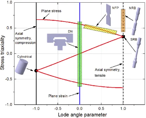
As far as the specimen geometry is concerned, when combined with the loading conditions, it should be able to reproduce several states of stress and strain rates usually found in metal cutting. There are two solutions to generate different states of stress in the specimens during the mechanical tests. One is to use advanced machines allowing complex multi-axial loadings to be performed with simple designed specimens [29]. The other solution is to use (complex) specially designed specimens to get the desired state of stress by applying simple loadings (tensile, compressive, torsion). The latter solution is relatively simple because the loading conditions are easier to control and the gauge areas are fixed. The aim of specimen design is to achieve the capability to generate a broad range of states of stress. Figure 3 shows the possible states of stress generated by combining several specimen geometries and loading types (tensile/compression) used in this work. The cylindrical specimen, double notch (DN), notched round bar (NRB), smooth round bar (SRB) and notched flat plate (NFP) specimens permitted several states of stress levels to be generated by varying their geometries. The values of state of stress were determined by the simulation of mechanical tests using all the specimens. The details of the simulations are discussed in the following text.

Fig. 3: States of stress and corresponding specimen geometries (cylindrical specimen; DN – double notched; NRB – notched round bar; SRB – smooth round bar; NFP – notched flat plate).

Figure 4 shows the axisymmetric specimen (cylindrical, SRB and NRB) geometries. The

cylindrical specimen (Figure 4a) was used in the compression tests at different strain rates, with a constant state of stress (stress triaxiality equals -1/3 and Lode angle parameter equals -1 for quasi-static conditions) [18]. Before designing other specimen geometries, quasi-static compression tests of cylindrical specimens were performed to obtain the flow stress. Then, this flow stress was applied in the simulations of the mechanical tests of other specimen geometries to determine their states of stress.

(a) (b)

Fig. 4: Nominal geometry of the axisymmetric specimens: a) cylindrical specimen used in compression tests at several strain-rates; b) smooth and notched round bars used in quasi-static tensile tests.

In contrast, the SRB (Figure 4b) was used in the tensile tests under quasi-static conditions to obtain a stress triaxiality of 1/3 and a Lode angle parameter of 1[18]. The NRB (Figure 4b) was introduced to generate values of stress triaxiality between 0.33 and 0.90, keeping the Lode angle parameter constant and equal to 1 [18]. The stress triaxiality values of these specimens in the center of the neck region can be estimated by Equation (11) [18].

center

1

ln 1

3

2

a

R



= +



_

+



_





a represents the minimum radius of the neck cross section and R represents the local radius of

the neck, as shown in Figure 4b. To vary the stress triaxiality from 0.33 to 0.90, three values of

R were used (6, 12 and 30), keeping the diameter of the neck cross-section constant at 6 mm.

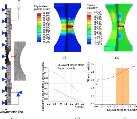
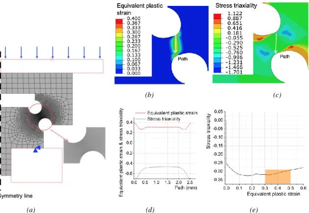
The value of stress triaxiality was evaluated by simulations of the mechanical tests. Fig. 5 shows an example of simulating a tensile test of notched round bar with R equal to 12 mm. Fig. 5a illustrates the model and the corresponding boundary conditions. To describe the material plasticity in this simulation, the stress-strain curves (before damage initiation) acquired from the quasi-static compression test of cylindrical specimens were used. The two extremities of the bar were fixed to a rigid body representing the machine clamping system. The bottom extremity of the bar was fixed, while the upper one moved at a constant loading speed of 1 mm/s. The 4-node axisymmetric elements (CAX4R) were applied in Abaqus/Explicit, and the minimum element size was 0.2 mm x 0.3 mm. Fig. 5b and Fig. 5c show the distributions of the equivalent plastic strain and the stress triaxiality, respectively, when the value of maximum equivalent plastic strain in the bar reaches 0.4. This strain limit was chosen since, according to Allahverdizadeh [30], the strain at damage initiation for Ti6Al4V alloy under different states of stress is in the range between 0.3 and 0.5. Fig. 5d shows the evolution of the equivalent plastic strain and the stress triaxiality from the center to the border of the specimen (in the direction of x axis). Since their values are largest in the center, this location is considered as the damage initiation point. Then, the stress triaxiality was plotted as a function of the equivalent plastic strain in this location (Fig. 5e). Analyzing this figure, the value of stress triaxiality varies between 0.72 and 0.89 when the strain at damage initiation is between 0.3 and 0.5 [30]. The stress triaxiality for the other specimen geometries was evaluated using similar methodology.

(a) (d) (e)

Fig. 5: Simulation of the tensile tests of NRB_R12: a) FE model with boundary conditions; b) distribution of the equivalent plastic strain; c) distribution of the stress triaxiality; d) distribution of the equivalent plastic strain and stress triaxiality in the direction of x axis; e) Relation between the stress triaxiality and the equivalent plastic

strain in the center of the bar.

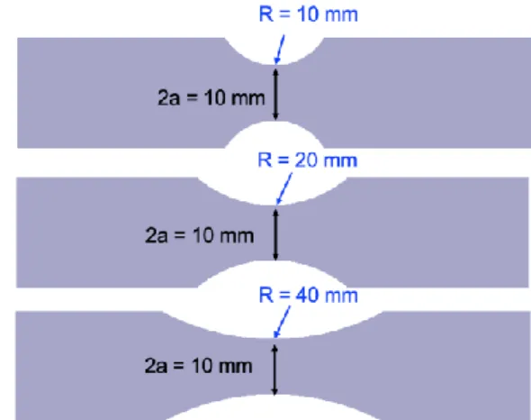
The notched flat plate (NFP) geometry was used to obtain the state of stress values under plane stress condition, as shown in Fig. 6. In this case, by varying the neck radius (R), different values of stress triaxiality and Lode angle parameter are generated. There were three types of notched flat plate: NFP_R10 (R = 10 mm), NFP_R20 (R = 20 mm) and NFP_R40 (R = 40 mm). The thickness of all these specimens was 2.35 mm to ensure plane stress conditions.

The same methodology as applied for the notched round bars was also applied to evaluate the values of two states of stress parameters for the notched flat plate. An example of notched flat plate with R equal to 10 mm is presented in Fig. 7. Half of the specimen geometry and the corresponding boundary conditions used in the model are shown in Fig. 7a. To describe the material plasticity in this simulation, the stress-strain curves (before damage initiation) acquired from the quasi-static compression test of cylindrical specimens were used. 3D elements (C3D8R) were used, with a minimum element size of 0.3 mm x 0.6 mm x 0.78 mm. Fig. 7b

(b) (c)

and Fig. 7c show the distributions of the equivalent plastic strain and the stress triaxiality, respectively. These distributions were obtained when the value of maximum equivalent plastic strain in the plate was equal to 0.4. Fig. 7d shows the evolution of the stress triaxiality and the equivalent plastic strain from the center to the border (in the direction of x axis). It is found that the largest value of stress triaxiality is located at the center of this specimen. Thererfore, the stress triaxiality was plotted as a function of the equivalent plastic strain in this location, where the largest stress triaxiality is obtained. The range of stress triaxiality varies between 0.59 and 0.74 when the strain at damage initiation is between 0.3 and 0.5 [30]. As far as the Lode angle parameter is concerned, the corresponding values are between -0.08 and -1 (yellow region in

Fig. 3).

Fig. 6: Nominal geometry of the notched flat plates applied in quasi-static tensile tests. a is the half width of the necking cross section and R is the local radius of a neck in the notched flat plate.

Finally, to generate different stress triaxiality values keeping the Lode angle parameter zero (plane strain conditions), the double notched specimen introduced by Abushawashi et al. [28] was used in the compression tests. This specimen has the advantage of generating both negative and positive stress triaxiality values, whereas the flat grooved specimen used by Bai and Wierzbicki [18] in tensile tests can only generate positive stress triaxiality values.

Different stress triaxiality values generated by the double notched specimen (DN) in compression tests are generated by varying the pressure angle. This angle is between the line passing through the centers of the two arcs and the (horizontal) line normal to the loading force, as shown in Fig. 8. Three double notched specimens with different pressure angles are presented in this figure. However, five pressure angles were selected for this study: 30o, 45o, 60o, 90o and 120o (references DN_30, DN_45, DN_60, DN_90 and DN_120, respectively). A

is generated by a pressure angle greater than 90°. These pressure angles generate stress triaxialities values between –0.7 and +0.6. Additionally, the thickness of all these specimens was 25 mm to ensure plane strain conditions, so that the Lode angle parameter was zero.

(a) (d) (e)

Fig. 7: Simulation of tensile tests of NFP_10: a) FE model with boundary conditions; b) distribution of the equivalent plastic strain; c) distribution of the stress triaxiality; d) distribution of the equivalent plastic strain and

stress triaxiality in the direction of x axis; e) Relation between the stress triaxiality and the equivalent plastic strain in the center of the plate.

In order to determine the pressure angles that generate a broad range of stress triaxiality in the region between two arcs, simulations of the compression tests using specimens with different pressure angles were performed. For instance, Fig. 9 presents the simulation of the compression test of the DN_60. Fig. 9a shows the model of half of a specimen geometry and the corresponding boundary conditions. To describe the material plasticity in this simulation, the stress-strain curves (before damage initiation) acquired from the quasi-static compression test of cylindrical specimens were used. A 4-node axisymmetric element (CAP4R) was used, and the minimum element size was 0.07 mm x 0.1 mm. Fig. 9b and Fig. 9c show the distributions

(b) (c)

of the equivalent plastic strain and the stress triaxiality, respectively, when the value of maximum equivalent plastic strain in the specimen reaches 0.4. To find the exact location of maximum stress triaxiality, a line connecting the maximum equivalent plastic strain values between both arcs was drawn. Then, the distribution of stress triaxiality and the equivalent plastic strain were plotted along this line (Fig. 9d). As can be seen, the largest value of stress triaxiality is located in the middle of the two arcs. Therefore, the stress triaxiality was plotted as a function of the equivalent plastic strain in this location, and represented in Fig. 9e. This figure reveals that the value of stress triaxiality for this specimen is between -0.31 and -0.29.

(a) (b) (c)

Fig. 8: Nominal geometry of the double notched specimen used in quasi-static compression tests: a) pressure angle less than 90o_{; b) pressure angle 90}o_{; c) pressure angle greater than 90}o_.

The procedure described above permitted determination of the range of states of stress generated by each specimen geometry. This information is important to select suitable specimen geometries to cover the broad range of state of stress represented in Fig. 3. The exact state of stress value for each specimen will be calculated in section 4.5 after the coefficients of the proposed plasticity model have been determined. All the specimens came from the same Ti6Al4V block. Since even small variations in the specimen geometry may have a non-negligible influence on the results, the dimensions of all the specimens were measured before conducting the mechanical tests, and specimens outside tolerance were re-fabricated or rejected.

Pressure angle = 30o

∅₄ ∅4

6 m m

(a) (d) (e)

Fig. 9: Simulation of compression tests of DN_60: a) FE model with boundary conditions; b) distribution of the equivalent plastic strain; c) distribution of the stress triaxiality; d) distribution of the equivalent plastic strain and stress triaxiality along the line connecting the maximum equivalent plastic strain values between both arcs; e)

relation between stress triaxiality and equivalent plastic strain in the center of the path.

3.2 Experimental setup

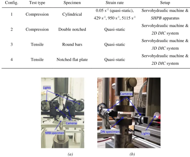
Table 2 displays four configurations of mechanical tests used in this study. Each test was

conducted twice to indicate the repeatability of the experimental data. Quasi-static (compression and tensile) tests of all specimen geometries were performed on a servohydraulic machine, while the compression tests of cylindrical specimens at different strain rates were performed using a Split Hopkinson Pressure Bar (SHPB) apparatus. To obtain the displacement or strain distribution on the specimen surface [31], a Digital Image Correlation (DIC) technique was applied in the quasi-static mechanical tests. Compared to strain gauges and extensometers, this is not affected by necking, which often complicates the determination of the strain at damage initiation. A 2D DIC system composed of a single CMOS camera and GOM software was applied for the planar specimens, such as double notched specimen and notched flat plates, while a commercial 3D DIC system from GOM composed of two CCD cameras and software was applied to the round bars due to the curved surface (Fig. 10b). Additionally, an extensometer was used in the tensile tests of round bars to measure the local displacement

(b) (c)

between two gauge points (Fig. 10a). Thus, the displacement was acquired by both 3D DIC and extensometer.

Table 2: Configurations of the mechanical tests.

Config. Test type Specimen Strain rate Setup

1 Compression Cylindrical 0.05 s

-1 _{(quasi-static),}

429 s-1_{, 950 s}-1_{, 5115 s}-1

Servohydraulic machine &

SHPB apparatus

2 Compression Double notched Quasi-static Servohydraulic machine &

2D DIC system

3 Tensile Round bars Quasi-static Servohydraulic machine &

3D DIC system

4 Tensile Notched flat plate Quasi-static Servohydraulic machine &

2D DIC system

(a) (b)

Fig. 10: Tensile and compression test setup of (a) NRB specimen and (b) DN specimen.

4. Determination of the constitutive model coefficients 4.1 Procedure for determination of the plasticity model coefficients

Fig. 11 shows the procedure to determine the plasticity model coefficients. The procedure

started with the first configuration shown in Table 2, used to determine the coefficients, A, B,

C, m, n and E, related to the strain hardening and strain rate effects. The quasi-static

compression test of a cylindrical specimen was defined as the reference test. Therefore, the reference coefficients used in the plasticity model were defined as: 𝜂0 = −1/3, 𝜀̇0 = 0.05 s-1

and 𝑐_θc = 1. Finally, the second and third configurations shown in Table 2 were used to determine the coefficients of the state of stress effect. The second configuration was used to

determine the coefficients c and 𝑐_θs, while 𝑐_θt and a were determined using the third configuration.

Fig. 12 shows the flowchart of the implementation of the optimization-based procedure in

Ls-Opt software, an optimization software module from LS-Dyna. First, a sort of initial model coefficients values were determined using a direct method, based on nonlinear least squares. These initial coefficients values were used to initialize the optimization-based procedure. D-optimal design was utilized to select the best set of coefficients. Then, these coefficients were used in the proposed constitutive model, which were imported into Abaqus/Explicit through a

VUMAT subroutine to simulate the mechanical tests. A metamodel was created based on the

simulated and experimental force-displacement curves. The difference between these two curves was evaluated by a curve mapping segment method [32]. In the next step, the difference was minimized by a hybrid algorithm, which used an adaptive simulated annealing (ASA) algorithm to find an approximate global solution, followed by Leapfrog Optimizer for Constrained Minimization (LFOP) algorithm to sharpen this solution [33]. Finally, a termination criterion including the force-displacement error and maximum number of iterations was checked. If it was not satisfied, a new response surface was built in the next iteration by the sequential response surface method (SRSM). The optimization-based process stopped when the termination criterion was satisfied, and the final coefficient values were obtained.

4.2 Young's modulus determination

The Young’s modulus needs to be known before determining the plasticity model coefficients. According to the Ti6Al4V alloy supplier, the Young’s modulus is between 107 and 122 GPa, and the Poisson’s ratio is 0.31. Then, quasi-static tensile tests of smooth round bars were performed to determine its exact value. The slope of stress-strain curve in the elastic region was measured, and the Young’s modulus found to equal 114 GPa.

4.3 Determination of the coefficients of the plasticity model

To determine the coefficients corresponding to the strain hardening and strain rate effects, compression tests of cylindrical specimens were performed at different strain rates of 0.05 s-1, 429 s-1, 950 s-1 and 5115 s-1. The force - displacement curves were obtained for each test, then the corresponding true stress-true strain curves were determined. Only the stress-strain curve before damage initiation was applied in the determination procedure. A compression test was also simulated by Abaqus/Explicit. Fig. 13 shows the model of half of the cylindrical specimen geometry and the corresponding boundary conditions. A mesh composed of 0.3 mm 4-node axisymmetric elements (CAX4R) was used. The friction coefficient between upper and bottom dies and specimen was 0.12, obtained using the ring compression test method. The loading speed (V) for different strain rates was determined by Equation (12) and applied to the upper die, while the bottom die was static.

*

V = h (12)

In this equation, 𝜀̇ is the strain rate and h is the specimen height.

Since the quasi-static compression test of a cylindrical specimen is the reference test, Equation

(4) is reduced to the first two terms (Equation (A) in Fig.11), i.e., the strain hardening and strain

rate effects. Applying the optimization procedure represented in Fig. 11, the values of the coefficients were modified iteratively to minimize the difference between the experimental and the simulated force-displacement curves for all the strain rates. Fig. 14a shows both simulated and experimental force-displacement curves after applying the optimization procedure. Fig.

14b shows both experimental true stress-true strain curves and the stress surface, the latter

calculated considering only the first two terms of Equation (4) and using the determined coefficients. It is seen that the stress surface matches quite well with the experimental data represented by the red dots. The determined coefficient values are summarized in Table 3.

(a) (b)

Fig. 14: a) Simulated and experimental force–displacement curves of the compression tests over cylindrical specimens after applying the optimization procedure; b) Experimental true stress – true strain curves and the stress surface calculated considering the first two terms of Equation (4) and using the determined coefficients.

As shown in Fig. 10, the next step consisted of determining the coefficients 𝑐_η and 𝑐_θs, related to the state of stress effect, using the double notched specimens. Five pressure angles of 30o_,

45o_{, 60}o_{, 90}o _{and 120}o _{were submitted to compression tests under the same quasi-static loading}

conditions, and the corresponding force-displacement curves were obtained. Applying the same optimization procedure described above and represented in Fig. 11, 𝑐_η and 𝑐_θs coefficients were determined, and are shown in Table 3. Fig. 15a shows both simulated and experimental force-displacement curves after applying the optimization procedure.

Finally, to determine the remaining coefficients related to the state of stress effect, 𝑐_θt and a, different notched round bars were used in the quasi-static tensile tests. The same minimum diameter of 6 mm was used with three different local neck radii R of 6 mm, 12 mm and 30 mm. Applying the same optimization procedure as described above and represented in Fig. 11, 𝑐_θt and a coefficients were determined, and are shown in Table 3. Fig. 15b shows both the simulated and experimental force-displacement curves after applying the optimization procedure.

Table 3: Determined coefficients of the plasticity model.

Strain hardening Strain rate Reference

Coefficient A m n B C E 𝜀̇0 𝜂0

Value 812.1 625.7 0.176 0.400 0.073 3949 0.05 -1/3

Stress triaxiality Lode angle

Coefficient 𝑐η 𝑐θs 𝑐θt 𝑐θc a

Value 0.212 0.795 1.061 1 4

(a) (b)

Fig. 15: Simulated and experimental force-displacement curves of: a) compression tests of double notched specimens; b) tensile tests of notched round bars.

4.4 Verification of plasticity model

After the determination of the plasticity model coefficients, simulations of the tensile tests of notched flat plates (fourth configuration in Table 2) were conducted to verify the accuracy of the plasticity model. It is worth pointing out that these specimens were not used in the

coefficient determination process. The model of the tensile test is almost the same as that in section 3.1, except for the plasticity model, which is replaced by the model given by Equation

(4) with the corresponding coefficients shown in Table 3. To estimate the contribution of each

effect on the flow stress, three simulations were performed corresponding to three plasticity models: 1) Equation (4) with the strain hardening (SH) and strain rate (SR) effects only; b)

Equation (4) with the SH, SR and stress triaxiality (Triax) effects; c) Equation (4) with all the

effects, including the Lode angle effect (Lode). Fig. 16 compares the simulated force-displacement curves with those measured for the NFP_R10 specimen.

Fig. 16: A comparison between simulated and experimental force–displacement curves for NFP_R10.

A large difference is observed (23%) between the simulated and experimental force-displacement curves when the plasticity model includes the strain and strain rate effects only. This difference is reduced to 4.1% when the stress triaxiality effect is also included in the plasticity model. Finally, the simulated force-displacement curve matches quite well with the experimental ones after also considering the Lode angle effect. The same influences of the strain hardening, strain rate, triaxiality and Lode angle on the force-displacement curves are observed for the other two notched flat specimens (NFP_R20 and NFP_R40). Therefore, it can be concluded that the state of stress effect, characterized by the stress triaxiality and the Lode angle, has a significant effect on the plasticity of Ti6Al4V titanium alloy.

the same time as the deformation process (before damage initiation), for both DN and NRB specimens. Fig.17 shows experimentally determined (by DIC) and simulated (FEM) strain distributions of these two types of specimen (DN with a pressure angle of 90º and NRB with a notch radius of 6 mm).

(a) (b)

Fig. 17. Equivalent plastic strain distribution in the DN (a) and NRB (b) before damage initiation, obtained by numerical simulation (left side) and determined by DIC (right side).

4.5 Determination of the coefficients of the damage model

Fig. 18 shows the procedure for the determination of the coefficients of Equation (8),

corresponding to damage initiation. First, experimental mechanical tests using all the specimen geometries were conducted and the corresponding force-displacement curves obtained. Numerical simulations of these mechanical tests were also performed to obtain the corresponding simulated force-displacement curves. Second, simulated and experimental curves for each test were compared, and the displacement at damage initiation di was obtained.

Third, the images taken by the DIC system cameras corresponding to the displacement at damage initiation were selected for DIC analysis, in order to calculate the equivalent plastic strain at damage initiation, 𝜀̅_ip. Knowing 𝜀̅_ip, the stress triaxiality η and Lode angle parameter 𝜃̅ can be obtained from the numerical simulations when the damage is initiated [23]. Using both equivalent plastic strain at damage initiation and state of stress, the coefficients of Equation (8) were determined.

To illustrate this procedure, the example of DN_90 is used in the compression tests (Fig. 19a) and numerical simulations (Fig. 19b). The displacement at damage initiation was determined by comparing the simulated and experimental force-displacement curves, as shown in Fig. 19c. This figure shows that the two curves have identical evolution until a displacement of 0.75 mm, then they follow different directions. Taking this value as the displacement at damage initiation, the corresponding strain at damage initiation 𝜀̅_ip can be obtained by analyzing the distribution of equivalent plastic strain in the specimens, determined experimentally using the DIC technique, as illustrated in Fig. 15a. The value of 𝜀̅_ip is the average of the two maximum values shown in this figure, and is equal to 0.275.

Fig. 18: Flowchart of the procedure for the determination of the damage initiation coefficients.

To determine the stress triaxiality at damage initiation, the distribution of equivalent plastic strain obtained from the simulation was used, as shown in Fig. 19b. In this figure, a path corresponding to a straight line crossing the regions of maximum equivalent plastic strain was drawn. Plotting both simulated equivalent plastic strain and stress triaxiality along this path (Fig. 19d), the stress triaxiality at damage initiation can be determined. It is located in the

this specimen due to the plane strain conditions. However, the exact value of the Lode angle parameter is not known for the notched flat specimen. Therefore, after knowing the location of damage initiation, which corresponds to the maximum value of stress triaxiality, the value of the Lode angle parameter was determined at the same location.

(a) (b)

(c) (d)

Fig. 19: Simulated and experimental results for DN_90: a) experimental strain distribution at damage initiation obtained by DIC; b) simulated strain distribution at damage initiation; c) simulated and experimental force-displacement curves; d) distribution of equivalent plastic strain and stress triaxiality along the selected path in a).

The same procedure was applied to the other specimens to get the state of stress (η and θ) and the equivalent plastic strain (𝜀̅_ip) at damage initiation. All the values are summarized in Table

4, and the 3D fracture locus was built in the space of (𝜀̅_ip, 𝜂, 𝜃̅), as shown in Fig. 20.

Fig. 20: Fracture surface of the Ti6Al4V alloy.

Table 4: A summary of the strains at damage initiation for all the specimens

Type of specimen Strain at damage initiation, 𝜀̅_ip Stress triaxiality, 𝜂 Lode angle parameter, 𝜃̅

Cylindrical 0.435 -0.333 -1 DN_30 0.423 -0.709 0 DN_45 0.457 -0.696 0 DN_60 0.37 -0.458 0 DN_90 0.277 -0.08 0 NRB_R6 0.384 0.976 1 NRB_R12 0.435 0.763 1 NRB_R30 0.476 0.623 1 NFP_R10 0.306 0.427 0.971 NFP_R20 0.545 0.487 0.922 NFP_R40 0.489 0.479 0.947

A wide range of state of stress is covered by the designed specimens, where the stress triaxiality varies from -0.709 to 0.976 and the Lode angle parameter varies from -1 to 1. According to Bai and Wierzbicki [18], boundary limits can be used to construct the fracture surface. Thus, three limiting cases are proposed: 𝜃̅ = −1, corresponding to the compression tests of cylindrical specimens; 𝜃̅ = 0, corresponding to the compression tests of double notched specimens; 𝜃̅ = 1, corresponding to the tensile tests of notched round bars. For each boundary limit, an exponential function was applied to characterize the relation between the strain at damage

determine the coefficients by fitting all the experimental points into the formulation of the damage initiation presented in Equation (8). Thus, three boundary limits were determined independently. First, D3, D4 and D5, D6 were determined by fitting the experimental points into

boundary limits 𝜃̅ = 0 and 𝜃̅ = 1, respectively. Secondly, the remaining experimental points were used to determine the coefficients D1, D2 related to the boundary line 𝜃̅ = −1. Finally,

the compression tests of the cylindrical specimens at different strain rates were used to determine D7 coefficient associated with the strain rate effect. All the determined damage model

coefficients are shown in Table 5.

Table 5: Determined coefficients of the damage model.

Damage coefficients D1 D2 D3 D4 D5 D6 D7

0.694 0.608 0.263 0.734 0.430 0.040 -0.028

In the case of the damage evolution, both the exponent parameter , and the fracture energy density Gf, were determined by applying the optimization procedure mentioned above. Only

the simulated and experimental force-displacement curves of the compression tests of double notched specimens were used. Fig. 21 illustrates the comparison between simulated and experimental force displacement curves after optimization, corresponding to Gf and  equal to

18.5 KJ/m2 and 9.4, respectively. After this optimization, the difference of fracture displacement between the simulation and the experimental test is 9% in the compression test of

DN_45, and smaller for the other two specimens. Moreover, the experimentally determined (by

DIC) and simulated plastic strain distributions in the specimens after damage initiation were also compared for specimens DN_90 and NRB_R6. As can be seen in Fig. 22, the simulated and experimental distributions are nearly identical. Therefore, the damage evolution process is predicted well by the proposed damage model.

Fig. 21: FE force–displacement response for double notched specimens compared to the experiments with damage evolution model.

(a) (b)

Fig. 22. Equivalent plastic strain distribution in the DN (a) and NRB (b) after damage initiation, obtained by numerical simulation (left side) and determined by DIC (right side).

5. Comparison of the proposed model and the Johnson-Cook model

To evaluate the precision of the proposed model to represent the mechanical behavior of the Ti6Al4V alloy in metal cutting, true stress-true strain curves obtained by this model were

in the finite element analysis of the metal cutting process. J-C plasticity and damage models are given by Equation (13) – (16), without the thermal softening term.

(

)

(

)







(

1 D

)



= −



Ajc, Bjc, Cjc and njc are the coefficients of the plasticity model, and 𝜀̇₀ is the reference strain rate

which equals 0.05 s-1. D1jc – D4jc are the damage coefficients and Gf is the fracture energy

density. 𝜀̅i is the plastic strain at damage initiation and 𝜀̅f is the plastic strain when all the

stiffness and fracture energy of the material have been lost and dissipated, respectively. 𝜎̃ is the hypothetical undamaged stress evaluated by Equation (13), 𝑙 is the characteristic length of the finite element in the simulation. 𝜇̅ = 0 is the equivalent plastic displacement before damage initiation while 𝜇̅_f is the equivalent plastic displacement at complete fracture.

The coefficients of the J-C model were also determined using the mechanical tests data. Compression tests of cylindrical specimens at different strain rates were used to determine the coefficients of the plasticity model (Ajc, Bjc, Cjc and njc), and the damage model coefficient

related to the strain rate effect (D4jc). Compression tests of double notched specimens were used

to determine the damage model coefficients associated with the stress triaxiality effect (D1jc –

D3jc). The value of Gf, was already determined in section 4.5. Table 6 shows the determined

coefficients of the J-C constitutive model for the Ti6Al4V alloy. Then, the numerical simulations of the mechanical tests were conducted with the J-C model, and the results obtained were compared with those obtained by the proposed constitutive model, as well as the experimental data. Fig. 23 shows these results for four different specimen geometries that generate different states of stress: cylindrical specimen (C), double notched specimen having a

pressure angle of 90° (DN_90), notched flat plate specimen with R equal to 10 mm (NFP_R10) and notched round bar with R equal to 12 mm (NRB_R12).

Table 6: Determined coefficients of the J-C model.

Plasticity Damage

Coef. Ajc Bjc njc Cjc D1jc D2jc D3jc D4jc Gf (KJ/m2) 𝜀̇0 (s-1) Value 812 844 0.261 0.015 0.245 0.081 -1.276 -0.028 18.5 0.05

Fig. 23: A comparison of force-displacement curves from experimental data and simulated results with the proposed constitutive model and the J-C model: a) compression test of cylindrical specimens at a strain rate of 950 s-1_{; b) quasi-static compression test of DN_90; c) quasi-static tensile test of NFP_R10; d) quasi-static tensile}

test of NRB_R12.

Both the proposed and J-C constitutive models used in the simulations of the compression tests of the cylindrical specimen at a strain rate of 950 s-1 generate force-displacement curves that match the experimental ones quite well. However, when the J-C model is applied in the

notched flat plate and notched round bar, the predicted force-displacement curves are considerably overestimated. In particular, higher forces and displacements at fracture were obtained using the J-C model, when compared to the proposed constitutive model and the experimental results. Therefore, the J-C model is not able to represent the mechanical behavior of Ti6Al4V alloy under different states of stress, while the proposed model shows good accuracy.

6. Conclusions

A constitutive model describing the mechanical behavior of Ti6Al4V titanium alloy that includes both the plasticity and damage is proposed. It accounts for the effects of strain hardening, strain-rate and the state of stress in both the plasticity and damage regions. This model can be used to describe the work material behavior in manufacturing process simulations involving crack propagation and neglecting the thermal effects on the mechanical behavior. This is the case for work material in the first deformation zone in metal cutting, where its separation from the workpiece is caused by crack propagation. Moreover, most of the heat produced due to plastic deformation in this zone flows into the chip, and only a small amount flows into the workpiece.

Numerical simulations of the tensile and compression tests with several specimen geometries permitted the state of stress (stress triaxiality and the Lode angle parameter) representative of the metal cutting process to be obtained. Then, experimental mechanical tests were conducted and the force–displacement curves obtained were used in a hybrid numerical/experimental optimization-based procedure to determine the constitutive model coefficients.

Additional force-displacement curves from mechanical tests of specimen geometries not used in the determination of coefficients procedure were obtained. The comparison between these experimental curves and the simulated ones (using the proposed constitutive model with the determined coefficients) confirmed the accuracy of the proposed constitutive model to describe the mechanical behavior of Ti6Al4V alloy under different states of stress. The accuracy was also confirmed by a benchmark test considering the proposed constitutive model and the J-C model. These simulations show the importance of the stress triaxiality and the Lode angle in the improvement of constitutive model accuracy.

Acknowledgements

The authors would like to express their gratitude for the financial support provided by Seco Tools and Safran companies. The financial support from French Ministries of Europe and Foreign Affairs (MEAE) and of Higher Education, Research and Innovation (MESRI), through the PHC PROCOPE program (project N°37773QM), as well as from the China Scholarships Council program (No. 201606320213) are also appreciated. They would like to thank Dr. Betrand Marcon from Arts & Metiers Paristech, Prof. Stefan Dietrich from Karlsruhe Institute of Technology and Prof. Pedro Rosa from University of Lisbon for their help in the mechanical tests. They would like also to thank Mr. Francois Auzenat from Seco SECO Tools and Dr. Lamice Denguir for their valuable contribution in commenting the results.

References

[1] Leyens, C., Peters, M., 2003. Titanium and titanium alloys: fundamentals and applications. John Wiley & Sons.

[2] M'Saoubi, R., Outeiro, J., Chandrasekaran, H., Dillon Jr, O.W., Jawahir, I.S., 2008. A review of surface integrity in machining and its impact on functional performance and life of machined products. International Journal of Sustainable Manufacturing 1(1-2), 203–236.

[3] Outeiro, J., Umbrello, D., M'Saoubi, R., Jawahir, I.S., 2015. Evaluation of present numerical models for predicting metal cutting performance and residual stresses. Machining Science and Technology 19(2), 183–216.

[4] Melkote, S.N., Grzesik, W., Outeiro, J., Rech, J., Schulze, V., Attia, H., Arrazola, P.-J., M'Saoubi, R., Saldana, C., 2017. Advances in material and friction data for modelling of metal machining. CIRP Annals - Manufacturing Technology 66(2), 731–754.

[5] Hibbit, H. D., Karlsson, B. I., & Sorensen, E. P, 2017. ABAQUS user manual, version 6.12. Simulia, Providence, Rhode Island.

[6] Johnson, G.R., Cook, W.H., 1985. Fracture characteristics of three metals subjected to various strains, strain rates, temperatures and pressures. Engineering Fracture Mechanics 21(1), 31–48.

[7] Meyer Jr, H.W., Kleponis, D.S., 2001. Modeling the high strain rate behavior of titanium undergoing ballistic impact and penetration. International Journal of Impact Engineering 26 (1-10), 509–521.

[8] Lee, W.S., Lin, C.F., 1998. High-temperature deformation behaviour of Ti6Al4V alloy evaluated by high strain-rate compression tests. Journal of Materials Processing Technique 75(1-3), 127–136.

[9] Leseur, D., 1999. Experimental investigations of material models for Ti-6A1-4V and 2024-T3. Lawrence Livermore National Laboratory (LLNL), Livermore, CA.

[10] Calamaz, M., Coupard, D., Girot, F., 2008. A new material model for 2D numerical simulation of serrated chip formation when machining titanium alloy Ti–6Al–4V. International Journal of Mechanical Sciences 48(3-4), 275–288.

[11] Sima, M., Özel, T., 2010. Modified material constitutive models for serrated chip formation simulations and experimental validation in machining of titanium alloy Ti– 6Al–4V. International Journal of Mechanical Sciences 50(11), 943–960.

[12] Dos Santos, T., Outeiro, J.C., Rossi, R., Rosa, P., 2017. A New Methodology for Evaluation of Mechanical Properties of Materials at Very High Rates of Loading. Procedia CIRP 58, 481–486.

[13] Follansbee, P.S., Kocks, U.F., 1988. A constitutive description of the deformation of copper based on the use of the mechanical threshold stress as an internal state variable. Acta Metallurgica 36(1), 81–93.

[14] Melkote, S.N., Liu, R., Fernandez-Zelaia, P., Marusich, T., 2015. A physically based constitutive model for simulation of segmented chip formation in orthogonal cutting of commercially pure titanium. CIRP Annals - Manufacturing Technology 64(1), 65–68. [15] Rotella, G., Umbrello, D., 2014. Finite element modeling of microstructural changes in

dry and cryogenic cutting of Ti6Al4V alloy. CIRP Annals - Manufacturing Technology 63(1), 69–72.

[16] Astakhov, V., 1998. Metal cutting mechanics. Boca Raton: CRP Press.

[17] Rice, J.R., Tracey, D.M., 1969. On the ductile enlargement of voids in triaxial stress fields. Journal of the Mechanics and Physics of Solids 17(3), 201–217.

[18] Bai, Y., Wierzbicki, T., 2008. A new model of metal plasticity and fracture with pressure and Lode dependence. International Journal of Plasticity 24, 1071–1096.

[19] Bai, Y., Wierzbicki, T., 2009. Application of extended Mohr–Coulomb criterion to ductile fracture. International Journal of Fracture 161(1), 1–20.

[20] Hillerborg, A., Modéer, M., Petersson, P.E., 1976. Analysis of crack formation and crack growth in concrete by means of fracture mechanics and finite elements. Cement and Concrete Research 6(6), 773–781.

[21] Buchkremer, S., Wu, B., Lung, D., Münstermann, S., Klocke, F., Bleck, W., 2014. FE-simulation of machining processes with a new material model. Journal of Materials Processing Technique 214(3), 599–611.

[22] Denguir, L., Outeiro, J., Fromentin, G., Vignal, V., Besnard, R., 2017. A physical-based constitutive model for surface integrity prediction in machining of OFHC copper. Journal of Materials Processing Technique 248, 143–160.

[23] Abushawashi, Y.M., 2013b. Modeling of metal cutting as purposeful fracture of work material. PhD thesis, Michigan State University.

[24] Wang, B., Liu, Z., 2016. Evaluation on fracture locus of serrated chip generation with stress triaxiality in high speed machining of Ti6Al4V. Materials and Design 98, 68–78. [25] Liu, J., Bai, Y., Xu, C., 2014. Evaluation of Ductile Fracture Models in Finite Element

Simulation of Metal Cutting Processes. Journal of Manufacture Science and Engineering 136(1), 011010–14.

[26] Abushawashi, Y.M., Xiao, X., Astakhov, V., 2012. Heat conduction vs. Hear advection in metal cutting. International Journal of Advances in Machining and Forming Operations 4(2), 122–151.

[27] Cheng, W., Outeiro, J., Costes, J.P., M'Saoubi, R., Karaouni, H., Denguir, L., Astakhov, V., Auzenat, F., 2018. Constitutive model incorporating the strain-rate and state of stress effects for machining simulation of titanium alloy Ti6Al4V. Procedia CIRP 77, 344–347. [28] Abushawashi, Y.M., Xiao, X., Astakhov, V., 2013a. A novel approach for determining material constitutive parameters for a wide range of triaxiality under plane strain loading conditions. International Journal of Mechanical Sciences 74, 133–142.

[29] Dunand, M., Mohr, D., 2011. Optimized butterfly specimen for the fracture testing of sheet materials under combined normal and shear loading. Engineering Fracture Mechanics 78(17), 2919–2934.

[30] Allahverdizadeh, N., Gilioli, A., Manes, A., Giglio, M., 2015. An experimental and numerical study for the damage characterization of a Ti–6AL–4V titanium alloy. International Journal of Mechanical Sciences 93, 32–47.

[31] Su, C., Anand, L., 2003. A new digital image correlation algorithm for whole-field displacement measurement. Massachusetts Institute of Technology, In: Proceedings Singapore-MIT Alliance Symposium of Innovation in Manufacturing Systems and Technology.

[32] Witowski, K., Feucht, M., Stander, N., 2011. An effective curve matching metric for parameter identification using partial mapping. 8th European LS-DYNA, Users Conference Strasbourg, 1–12.

[33] Stander, N., ROUX, W., Eggleston, T., Craig, K., 2007. LS-OPT users’ manual–a design optimization and probabilistic analysis tool for the engineering analyst. Livermore Software Technology Corporation, Livermore.