Ductility prediction of substrate-supported metal layers based on rate-independent crystal plasticity theory

Science Arts & Métiers (SAM)

is an open access repository that collects the work of Arts et Métiers Institute of

Technology researchers and makes it freely available over the web where possible.

This is an author-deposited version published in: https://sam.ensam.eu Handle ID: .http://hdl.handle.net/10985/19115

To cite this version :

Holanyo K. AKPAMA, Mohamed BEN BETTAIEB, Farid ABED-MERAIM - Ductility prediction of substrate-supported metal layers based on rate-independent crystal plasticity theory - In: NUMIFORM 2016: The 12th International Conference on Numerical Methods in Industrial Forming, France, 2016-07 - MATEC Web of Conference-Numiform2016 - 2016

Any correspondence concerning this service should be sent to the repository Administrator : archiveouverte@ensam.eu

a

Corresponding author: Mohamed.BenBettaieb@ensam.eu

independent crystal plasticity theory

Holanyo K. Akpama1, Mohamed Ben Bettaieb1,2, a and Farid Abed-Meraim1,2 1

LEM3, UMR CNRS 7239 - Arts et Métiers ParisTech, 4 rue Augustin Fresnel, 57078 Metz Cedex 3, France

2_{DAMAS, Laboratory of Excellence on Design of Alloy Metals for low-mAss Structures, Université de Lorraine, France}

Abstract. In this paper, both the bifurcation theory and the initial imperfection approach are used to predict localized necking in substrate-supported metal layers. The self-consistent scale-transition scheme is used to derive the mechanical behavior of a representative volume element of the metal layer from the behavior of its microscopic constituents (the single crystals). The mechanical behavior of the elastomer substrate follows the neo-Hookean hyperelastic model. The adherence between the two layers is assumed to be perfect. Through numerical results, it is shown that the limit strains predicted by the initial imperfection approach tend towards the bifurcation predictions when the size of the geometric imperfection in the metal layer vanishes. Also, it is shown that the addition of an elastomer layer to a metal layer enhances ductility.

1 Introduction

The ductility of a material is characterized by its ability to deform homogeneously under some imposed loading. For sheet metals undergoing in-plane biaxial loading, at a certain limit strain, the deformation starts concentrating in narrow bands. The occurrence of such localization bands marks the onset of localized necking in the sheet. Predicting the different limit strains that lead to localized necking is crucial for designing functional or structural components used in industrial devices. To this end, several numerical models have been developed to predict localized necking, which is represented in the form of forming limit diagram (FLD). This FLD concept was initially introduced by Keeler and Backofen [1], for representing the limit strains in the range of positive strain paths, and has been extended by Goodwin [2] to the range of negative strain paths. Despite the wide range of FLD prediction models available in the literature, very few of them have been devoted to metal/elastomer bilayers. However, the latter have proven better stretchability than traditional freestanding metal layers, and are being increasingly used in the industry. For instance, in the design of electronic devices that require high levels of stretchability, substrate-supported metal layers are often used. This is the case of stretchable conductors used in biomedical applications, and interconnects that are used in large-scale integrated circuits [3,4]. The current paper proposes an efficient tool for the prediction of localized necking in substrate-supported metal layers. The mechanical behavior of a representative volume element of the metal layer is determined from the mechanical behavior of its microscopic constituents by using the self-consistent

scale-transition scheme. Such a micromechanical approach allows an accurate description for the mechanical behavior of the metal layer. Indeed, the

self-consistent model takes into account essential

microstructure-related features that are relevant at the microscale. These microstructural aspects include key physical mechanisms, such as initial and induced crystallographic textures, morphological anisotropy, and interactions between grains and their surrounding medium. The mechanical behavior at the single crystal scale is described by a finite strain rate-independent constitutive framework, where the Schmid law is used to model the plastic flow. This rate-independent formulation is more suitable for the modeling and the simulation of cold forming processes, where viscous effects are limited. The developed model is applied in this paper to metal layers with FCC crystallographic structure. On the other hand, the mechanical behavior of the elastomer layer is assumed to obey the hyperelastic neo-Hookean constitutive law. The adherence between the two layers is assumed to be perfect. In order to predict localized necking in the bilayer, the overall mechanical behavior is coupled with two different localization criteria: the bifurcation theory, initially developed by Rice [5], and the imperfection approach initiated by Marciniak and Kuczynski [6]. The use of the Schmid law at the single crystal scale allows predicting limit strains at realistic levels when the bifurcation theory is used as localization criterion. One of the main conclusions of this paper is that the addition of an elastomer layer can significantly retard the occurrence of localized necking in the whole bilayer. It is also demonstrated that the FLDs of the bilayer predicted by the Marciniak–Kuczynski (MK)

NUMIFORM 2016

analysis tend towards those predicted by the bifurcation theory in the limit of a vanishing size for the geometric imperfection of the metal layer.

The current paper may be viewed as an extension of the investigations carried out in [7], which were restricted to a phenomenological description for the mechanical behavior of the metal layer.

The remainder of the paper is organized as follows: - The constitutive equations describing the mechanical behavior of the metal and elastomer layers will be outlined in the second section.

- In the third section, the theoretical framework for the two localization criteria will be presented.

- Various numerical results obtained by the application of the developed tool will be presented and discussed in the fourth section.

Notations

The following notations and abbreviations are adopted in this paper:

- Mechanical fields corresponding to the polycrystal (resp. single crystal) scale are denoted by capital (resp. small) letters. To be consistent with the notations adopted for the metal layer, the different mechanical fields corresponding to the elastomer layer are also denoted by capital letters.

- PS: the in-plane part of the field  (in relation with the plane-stress assumption).

- : quantity  associated with layer  (metal or elastomer layer).

- (B): quantity  associated with the band (MK analysis).

- (S): quantity  associated with the safe zone (MK analysis).

- SC and FC will be used, as needed, to specify the self-consistent scheme and the full-constraint Taylor model, respectively.

- FM (resp. BL) refers in figures of Section 4 to the freestanding metal layer (resp. metal/elastomer bilayer). These notations may be combined. For instance, tensor

X in the elastomer layer of the band is denoted X_E(B).

2 Mechanical behavior of the bilayer

2.1 Metal layer

2.1.1 Constitutive equations at the polycrystalline scale

Let us consider a polycrystalline aggregate, which is assumed to be statistically representative of the metal layer. The modeling of the mechanical behavior of this aggregate is thus sufficient to accurately describe the mechanical behavior of the whole metal layer. To derive the mechanical behavior of the polycrystalline aggregate from the behavior of its microscopic constituents, the self-consistent model is used. Only the main lines of this scheme are presented in the current section. Further details on this model are provided in [8]. Compared to the

full-constraint Taylor model, which is much more commonly used due to its simplicity, the self-consistent scheme presents a number of advantages. Indeed, through the formulation of this scale-transition scheme, the equilibrium condition at the single crystal level is satisfied. Also, the grain morphology and the interactions between the grain and its surrounding medium are accounted for.

Because the behavior of the polycrystalline aggregate is modeled within the framework of finite strains, the nominal stress rate N and the velocity gradient G are used as appropriate stress and strain measures, respectively. The macroscopic tangent modulus L

linking N to G is then obtained by using the self-consistent model

:



N L G. (1)

The macroscopic velocity gradient G and the nominal stress rate N can be derived from their microscopic counterparts g and n by using the averaging Hill theorem [9]

( ) ; ( )

 

G g x N n x , (2)

where

x

is a material point in the polycrystalline aggregate, and a the average of field a over the volume

V of the polycrystalline aggregate

1 ( ) d 

_

a a x x V V . (3)

Conversely, the microscopic velocity gradient and nominal stress rate are linked to their macroscopic counterparts by the following relations:

( ) ( ) : ; ( )  ( ) :

g x Α x G n x B x N, (4)

where Α x( ) and B x( ) are fourth-order concentration tensors for the velocity gradient and the nominal stress rate, respectively.

At the microscopic level, a behavior law similar to Eq. (1) can be derived by combining the constitutive relations of the single crystal

( )  ( ) : ( )

n x l x g x , (5)

where l is the microscopic tangent modulus.

Furthermore, it is assumed that all mechanical variables are homogeneous within the individual single crystals

g g N N 1 1 ( )



_ ( ) ; ( ) 



_ ( ) g x gI I x l x lI I x I θ I θ , (6)

where N_g is the number of single crystals that compose the polycrystalline aggregate, and θI is an indicator function defined as

( )x 1 if x ; ( )x 0 if x

I I I I

Thus, for any material point

x

within single crystal I, relation (5) becomes

:

nI lI gI_{. (8)}

The relation between L and l can be obtained by combining Eqs. (1)-(5)

L l x( ) :A x( ) (9)

By using Green’s tensor, the analytical expression of the concentration tensor AI _{is obtained after some}

developments

: 

 

            

AI Ι ΤII lI L Ι ΤII lI L _,(10)

where ΤII _{is a fourth-order tensor, which is function of} L, that describes the interaction between grain I and its surrounding medium. The macroscopic tangent modulus derived by the 1-site self-consistent version of the incremental scheme of Hill [9] can be finally obtained as follows: 1 :  



L Ng I Il AI I f , (11) where I

f is the volume fraction of single crystal I. The above equations (10) and (11) represent a non-linear problem, which is incrementally solved by using the iterative fixed point method. At each time increment, the main unknown of this iterative problem is the macroscopic tangent modulus L. It must be noted that the full-constraint Taylor model can be easily deduced from the self-consistent approach, by considering that the concentration tensors AI _{of the different grains are equal}

to the fourth-order identity tensor. In this particular case, no iteration is required. To calculate by Eq. (11), the microscopic tangent modulus lI _{of all individual grains}

should be computed. To this end, the following section is dedicated to the derivation of the analytical expression of the microscopic tangent modulus.

2.1.2 Constitutive equations at the single crystal scale

The mechanical behavior of the single crystals that make up the polycrystalline aggregate is described by a rate-independent constitutive framework. Because the single crystals undergo finite strains, the effect of lattice rotation is accounted for.

The microscopic velocity gradient is additively split into its symmetric and skew-symmetric parts, denoted as

d

and w , respectively

T T

1 2) ( ) ; 1 2) ( )

       

d g g w g g . (12)

The strain tensor d and the spin tensor w are split into their elastic and plastic parts

e p e p

    

d d d w w w . (13)

The rotation of the single crystal lattice frame

r

is related to the elastic part of the spin tensor we by the following relation:

T e

. 

r r w . (14)

In order to satisfy the objectivity principle, the co-rotational rate σ of the Cauchy stress tensor

σ

, with respect to the lattice rotation, is related to the elastic strain rate de by the following hypoelastic law:

e_{. .} e e _: e

 _{  }

σ σ w σσ w C d , (15)

where Ce is the fourth-order elasticity tensor. The elastic behavior of the metal layer is assumed to be isotropic and therefore Ce is defined by the Young modulus E and the Poisson ratio .

The inelastic deformation is only due to the slip on the crystallographic planes. Thus, p

d and p

w can be

defined by the following relations:

s s N N p p 1 sgn( ) ; 1 sgn( )   







d _β γβ

τ

β Rβ w _β γβ

τ

β Sβ,(16) where:

 N_s is the total number of slip systems (equal to 12 for FCC crystallographic structure).

 _{γ is the slip rate of the slip system β.} β

 Rβ (resp. Sβ) is the symmetric part (resp. skew-symmetric part) of the Schmid orientation tensor.

 _τβ _{is the resolved shear stress of the slip system β,}

which is equal to σ R: β.

The Schmid law is used to model the plastic flow of the single crystal, as follows:

c s c < = 0 1,..., N : = 0      _    β β β β β β τ τ γ β τ τ γ , (17) where c β

τ is the critical shear stress of the slip system β. The Cauchy stress tensor

σ

is related to the nominal stress tensor

n

by the following relation:

.

 

n jf σ, (18)

where j is the Jacobian of the microscopic deformation gradient f. The nominal stress rate n required in Eq. (5) can be easily obtained from Eq. (18)





. Tr ( ) .



  

n jf σ σ d g σ . (19)

In the current paper, an updated Lagrangian approach is adopted. Thus, in Eq. (19), f is set to the second-order identity tensor I₂ and j is set to 1, which reduces to

NUMIFORM 2016

Tr ( ) .

  

n σ σ d g σ. (20)

By combining Eqs. (12), (13), (15), (16) and (20), n

can be expressed as a function of the slip rates γ β









s e 2 N _e 1

sgn(

)

. .          



   n C σ I d σ w d σ C Rβ S σβ σ Sβ β β β _γ

τ

.(21)

Let us now introduce the set of active slip systems , defined as the slip systems for which the slip rates are strictly positive. The set of slip systems β used in Eq. (21) is then reduced to the set









e 2 e . .

sgn(

)

         



   n C σ I d σ w d σ C Rβ S σβ σ Sβ β β β _γ

τ

.(22)

In order to obtain the expression of the microscopic tangent modulus l from relation (22), the slip rates of the active slip systems γβ should be expressed as functions of g. To this end, the consistency condition, restricted to the active slip systems, is used

c

: sgn ) 0

 _β

_

  _{τ τ}β β _τβ    _γβ 

.(23) By using the definition of the resolved shear stress as well as Eqs. (13)1 and (15), the resolved shear stress rate

β

τ can be expressed as

e ₍ p₎

: :  : :

 β τβ Rβ σ Rβ C dd . (24)

As to the time derivative of τ_cβ, it is given by the following isotropic hardening law:

c 1 0 1 0 : 1 ;          _  _   





s β α α n N _α 0 α β τ h γ h h h γ τ n





, (25)

where h₀ is the initial hardening rate and n the power-law hardening exponent. τ₀ is the initial critical shear stress, which is assumed to be the same for the different slip systems.

The expression of the slip rates for the active slip systems is finally obtained by inserting Eqs. (16)1, (24)

and (25) into the consistency condition (23)

e sgn( ) : : : :     



 R C y

d

d

α βα α α β β _{M τ}

γ

, (26)

where M is the inverse of matrix P of rank Card( ), which is defined by the following index form:



e



: sgn( ) sgn( ) : :

,

  



α

β Pαβ h τα

τ

β Rα C Rβ

. (27)

Combining Eqs. (5), (21) and (26), one can obtain the analytical expression of the microscopic tangent modulus

l





e 1 2 2 e _{: . .}

( )

( )

sgn(

)

l C σ I σ σ C R S σ σ S y       



     α α α α α α

τ

,(28)

where 1 _and 2 _{are fourth-order tensors that reflect}

the contribution of Cauchy stress convective terms

1 2 1 (δ δ ) 2 1 (δ δ ) 2

( )

( )

σ σ     ijkl lj ik kj il ijkl ik lj il kj σ σ σ σ





.

(29)

In order to update the different microscopic variables, the above constitutive equations should be integrated incrementally over each time increment. Analyzing these constitutive equations, one can observe that the main unknowns are the set of active slip systems and the corresponding slip rates. An implicit ultimate algorithm, very similar to the one developed in [10], is used to integrate these equations. The microscopic tangent modulus is determined from the updated microscopic variables at the end of the time increment.

2.2 Elastomer layer

In contrast to the metal layer, the mechanical behavior of the elastomer layer is assumed to be homogeneous and is modeled by a hyperelastic neo-Hookean law [11]. The formulation of this model allows linking the Cauchy stress tensor Σ to the left Cauchy-Green tensor V

2 2

 

Σ qI V , (30)

where  is the shear modulus, q an unknown hydrostatic pressure to be determined by applying the incompressibility constraint, and V is defined by the following relation:

2 T

.



V F F , (31)

with F being the deformation gradient tensor of the elastomer layer.

3 Strain localization criteria

Let us consider a bilayer comprised of a metal layer M and an elastomer layer E. The two layers are assumed to be perfectly adhered and sufficiently thin. The small thickness assumption allows formulating the two above-mentioned localization criteria, namely the bifurcation theory and the initial imperfection approach, under the plane-stress conditions.

3.1 Bifurcation theory

The bilayer is submitted to uniform strain, where the in-plane strain rates are equal to E₁₁ 1, E₂₂  ρ and

12 0

E . ρ is the strain-path ratio ranging from 1/2 (uniaxial tensile state) to 1 (equibiaxial tensile state). Considering the plane-stress conditions, this specific loading implies that the macroscopic velocity gradient and the macroscopic nominal stress rate tensor have the following generic forms:

1 0 0 ? ? 0 0 0 ; ? ? 0 0 0 ? 0 0 0          _{ }  _{ }         G ρ N , (32)

where symbol ? designates the unknown components in both tensors. These generic forms are valid for both layers.

The bifurcation criterion states that strain localization occurs when the acoustic tensor becomes singular. Hence, this criterion is expressed in the following form:

PS PS PS

det ( .L . )0, (33)

where:

 PS _{is the unit vector normal to the localization band.}

Here, it is taken equal to (cos ,sin )  .

 PS

L is the averaged plane-stress tangent modulus of the bilayer. This modulus is defined by the following relation: PS PS M M E E PS M E    L L L h h h h , (34)

where h_M (resp. h_E)is the initial thickness of the metal (resp. elastomer) layer and PS

M

L (resp. PS

E

L ) is the plane-stress tangent modulus of the metal (resp. elastomer) layer.

PS M

L is derived from the 3D expression of the metal layer tangent modulus L_M (see Section 2.1.1) by using the following condensation relation:

M 33 M 33 PS M M M 3333 , , , 1 2 :, α β γ δ  L _αβγδ  L _αβγδ  L αβ L γδ L .(35) PS E

L is defined by the following relation [7]:

PS 1 2

E 2

( )

( )

L  ΣΙ  Σ   Σ , (36)

It is worth noting that the tensors 1 _and 2 _{used in}

relation (36) are given in Eq. (29). The non-zero components of the fourth-order tensor are defined by the following relations:

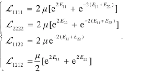
11 11 22 22 11 22 11 22 11 22 2 2 ( ) 1111 2 2 ( ) 2222 2 ( ) 1122 2 2 1212 [e e ] [e e ] e [e e ] 2        _{  }       _{ }   _{ }  E E E E E E E E E E μ μ μ μ . (37)

For each strain-path ratio , and at each time increment, the bifurcation criterion (33) is checked for all possible band orientations ( [0, /2]). When the acoustic tensor becomes singular for a given band orientation, the computation is stopped. The overall major strain E that is thus calculated corresponds to the ₁₁ localization limit strain and the band orientation, which zeroes the determinant of the acoustic tensor, corresponds to the necking band orientation.

3.2 Initial imperfection approach

In order to apply the initial imperfection approach (called hereafter M–K analysis for the sake of brevity) to the bilayer, the assumption of the preexistence of a groove in the form of a band in the metal layer (Figure 1) is made.

Thus, in accordance with various experimental

observations, the localization initiates always in the metal layer.

Figure 1. M–K analysis for a bilayer (initial geometry and band orientation).

In order to present the equations of the M–K analysis related to the metal/elastomer bilayer, the following notations are adopted:

 hM(B): initial thickness of the metal layer inside the

band.

 h_M(S): initial thickness of the metal layer outside the band.

 h_E(B): initial thickness of the elastomer layer inside the band.



hE(S): initial thickness of the elastomer layer outside

the band (equal to h_E(B)).

On the basis of these notations, the initial geometric imperfection ratio



₀ (corresponding to the metal layer only), can be specified as

M 0 M (B) 1 (S)  h h



. (38)

The M–K analysis is based on four main equations:

 As a consequence of the perfect adherence between the metal and the elastomer layer, the following equalities

NUMIFORM 2016

between the in-plane velocity gradients in the metal layer and their counterparts in the elastomer layer are satisfied: PS PS PS M E PS PS PS M E (B) (B) (B) (S) (S) (S)     G G G G G G (39)

 The kinematic compatibility condition between the band and the uniform zone (i.e., outside the band): this condition requires that the displacement increments should be continuous across the band and it is mathematically expressed as

PS PS PS PS

S

     

G G C . (40)

 The equilibrium balance across the interface between the band and the homogeneous zone:

PS PS PS M M E E PS PS PS M M E E .( (B) (B) (B) (B)) .( (S) (S) (S) (S))    Ν Ν Ν Ν h h h h . (41)

 The behavior law of both the metal and the elastomer layer, restricted to the plane dimension inside and outside the band, respectively: these constitutive equations are expressed in the following generic form:

PS PS PS PS PS PS M M E E PS PS PS PS PS PS M M E E (B) (B) (B) ; (B) (B) (B) (S) (S) (S) ; (S) (S) (S)     Ν L G Ν L G Ν L G Ν L G : : : : .(42)

By inserting the constitutive relations (42) into the equilibrium equation (41), this latter becomes

PS PS PS PS M M E E PS PS PS PS M M E E .( (B) (B) (B) (B)) : (B) .( (S) (S) (S) (S)) : (S)    L L G L L G h h h h . (43)

For each strain-path ratio ρ and each initial band orientation



₀, the equations that govern the MK approach are integrated incrementally over each time increment. Indeed, by analyzing Eqs. (40) and (43), it can be seen that the main incremental unknowns of the M–K approach are the two components of the jump vector PS

C

. For each loading (determined by a strain path and a band orientation), the computations are stopped when the norm of the jump vector CPS increases rapidly, thus marking the localization of the deformation in the band zone. Further numerical and algorithmic details regarding the M–K approach can be found in [7].

4 Prediction results

4.1 Material and geometric data

The polycrystalline aggregate studied in this paper is made of 2000 grains. Its initial crystallographic texture is generated randomly (see Figure 2) in such a way that it is orthotropic with respect to the rolling and transverse

directions. Initially, all of the grains are assumed to be spherical with the same volume fraction.

Figure 2. Initial crystallographic texture of the studied polycrystalline aggregate: {111} pole figure.

The material parameters of the single crystals are given in Table 1.

Table 1. Material parameters of the single crystals used in the metal layer

Elasticity Hardening E [GPa]  0 [MPa] h0 [MPa] n

210 0.3 40 390 0.35

The shear modulus of the elastomer layer is set to 22 MPa. The ratio between the initial thickness of the elastomer layer and the initial thickness of the metal layer is fixed to 0.5.

4.2 Bifurcation theory predictions

The evolution of the minimum of the cubic root of the determinant of the acoustic tensor PS .LPS. PS, over all possible band orientations, as a function of the major strain E₁₁ is displayed in Figure 3. The onset of strain localization occurs when this minimum reaches 0 as defined by the bifurcation criterion (33). The SC approach is used as scale-transition scheme. Four representative strain paths are considered in this figure: 

0.5, 0, 0.5, and 1. By comparing Figure 3 (a) and Figure 3 (b), one can easily observe that the presence of the elastomer layer substantially retards the occurrence of strain localization. This result is the consequence of the fact that under biaxial loading, the tangent modulus of the elastomer remains unchanged, or increases, while the tangent modulus of the metal layer steadily decreases.

RD

(a) (b)

Figure 3. Evolution of the minimum of the cubic root of the determinant of the acoustic tensor as a function of E11 for four different strain paths ( 0.5,  ,  0.5, and  ): (a) Freestanding metal layer; (b) substrate-supported metal layer.

The effect of the elastomer layer on necking retardation for all strain paths ρ [ 1/ 2, 1] is investigated in Figure 4. This figure, confirms the preliminary result obtained in Figure 3: the elastomer layer permits to shift the FLD monotonically upwards, and thus enhances the ductility of the bilayer.

(a) (b)

Figure 4. Effect of the elastomer layer on the improvement of the FLD of the bilayer: (a) SC model; (b) FC model.

4.3 M–K analysis predictions

In order to illustrate the onset of strain localization, the evolution of the in-plane components of the jump vector

C and the determinant of the acoustic tensor in the band are plotted in Figure 5 as function of the major strain in the safe zone E11. In this simulation, the strain path , the

initial imperfection ratio 0 and the initial band

orientation 0 are fixed to 0, 10 and 0°, respectively.

The SC model is used to ensure the transition between the microscopic and macroscopic scales of the metal layer. It is clear from Figure 5 (a) that the jump vector C remains very close to 0 before strain localization. This jump vector, and especially its first component, increases very abruptly when the strain in the safe zone E11 is about

0.28, thus leading to the localization of deformation within the band. The evolution of the determinant of the acoustic tensor in the band is given in Figure 5 (b). The limit strain (0.28) is reached when this determinant becomes equal to 0. This result is expectable considering the similarity in the mathematical formulation of the

bifurcation theory and the MK approach. The evolution of this determinant can be used as a reliable alternative indicator of strain localization for the different strain paths.

(a) (b)

Figure 5. Illustration of the onset of strain localization (bilayer;

 0; 0 103; 0 0°; SC): (a) Evolution of the in-plane components of the jump vector C as a function of the major strain in the safe zone E11; (b) Evolution of the determinant of the acoustic tensor in the band as a function of the major strain in the safe zone E11.

The comparison between the FLDs predicted by bifurcation theory and those determined by M–K analysis is shown in Figure 6. Three different values of the initial imperfection ratio 0 are considered: 104, 103 and 102.

It is clear that the shape and the level of the predicted FLDs are significantly influenced by the amount of initial geometric imperfection. It is also found that for all strain paths, the limit strains predicted by bifurcation theory set an upper bound to those yielded by the M–K approach. Moreover, this result is valid for both scale-transition schemes, namely the FC and SC models.

(a) (b)

Figure 6. Effect of the initial geometric imperfection on the shape and the level of the FLDs of the bilayer: (a) SC model; (b) FC model.

5 Concluding remarks

A powerful tool to predict the onset of localized necking in substrate-supported metal layershas been developed in this paper. In this tool, the mechanical behavior of the metal (resp. elastomer) layer is modeled by the self-consistent micromechanical model (resp. neo-Hookean hyperelastic model). The mechanical modeling of the bilayer is coupled with two strain localization criteria to

0.00 0.15 0.30 0.45 0.60 0 1x102 2x102 3x102 4x102 5x102     E 11   PS 1/3 PS_.PS_. PS Min _det L _ FM 0.0 0.2 0.4 0.6 0 1x102 2x102 3x102 4x102 5x102     E11   PS 1/3 PS_.PS_. PS Min det  BL -0.4 -0.2 0.0 0.2 0.4 0.0 0.2 0.4 0.6 0.8 E₂₂ E₁₁ FM BL FC -0.4 -0.2 0.0 0.2 0.4 0.0 0.2 0.4 0.6 0.8 E₂₂ E₁₁ FM BL SC 0.0 0.1 0.2 0.3 0.4 0 2 4 6 8 1 2 E₁₁ C C __ SC 0.0 0.1 0.2 0.3 0.4 0 2x102 4x102 6x102 8x102 1x103  _ SC  PS_.PS_(B). PS det L E11 -0.2 0.0 0.2 0.0 0.2 0.4 0.6 0.8   _ Bifurcation MK E₂₂ E₁₁ _ FC -0.2 0.0 0.2 0.0 0.2 0.4 0.6 0.8 SC Bifurcation  E₂₂ E₁₁      

NUMIFORM 2016

predict the limit strains: the bifurcation theory and the initial imperfection approach. From the numerical predictions obtained by applying this tool, three main conclusions can be drawn:

 The presence of an elastomer layer increases substantially the level of the limit strains for the bilayer.

 The shape and the level of the predicted FLDs are significantly influenced by the amount of initial geometric imperfection, which is assumed to initiate in the metal layer.

 The limit strains of the whole bilayer predicted by bifurcation theory set an upper bound to those yielded by the M–K approach.

References

1. S.P. Keeler, W.A. Backofen, Trans. ASM 56, 25 (1963)

2. G.M. Goodwin, Metallurgia Italiana 60, 767 (1968) 3. S.L. Chiu, J. Leu, P.S. Ho, J. Appl. Phys. 76, 5136

(1994)

4. M. Hommel, O. Kraft, Acta Mater. 49, 3935 (2001) 5. J.R. Rice, 14th International Congress of Theoretical

and Applied Mechanics, 207 (1976)

6. Z. Marciniak, K. Kuczynski, Int. J. Mech. Sci. 9, 609 (1967)

7. M. Ben Bettaieb, F. Abed-Meraim, Int. J. Plast. 65, 168 (2015)

8. P. Lipinski, M. Berveiller, E. Reubrez, J. Morreale, Arch. Appl. Mech. 65, 291 (1995)

9. R. Hill, Proc. Roy. Soc. London, 326, 131 (1972) 10. H.K. Akpama, M. Ben Bettaieb, F. Abed-Meraim,

Int. J. Num. Meth. Eng., doi: 10.1002/nme.5215 (2016)