Inverse and Direct Dynamic Modeling of Gough-Stewart Robots

(1)

HAL Id: hal-00401751

https://hal.archives-ouvertes.fr/hal-00401751

Submitted on 6 Jul 2009

HAL is a multi-disciplinary open access

archive for the deposit and dissemination of

sci-entific research documents, whether they are

pub-lished or not. The documents may come from

teaching and research institutions in France or

abroad, or from public or private research centers.

L’archive ouverte pluridisciplinaire HAL, est

destinée au dépôt et à la diffusion de documents

scientifiques de niveau recherche, publiés ou non,

émanant des établissements d’enseignement et de

recherche français ou étrangers, des laboratoires

publics ou privés.

Robots

Wisama Khalil, Sylvain Guegan

To cite this version:

Wisama Khalil, Sylvain Guegan. Inverse and Direct Dynamic Modeling of Gough-Stewart Robots.

IEEE Transactions on Robotics and Automation, Institute of Electrical and Electronics Engineers

(IEEE), 2004, 20 (4), pp.754-762. �hal-00401751�

(2)

Abstract--This paper presents closed form solutions for the

inverse and direct dynamic models of the Gough-Stewart parallel robot. The models are obtained in terms of the Cartesian dynamic model elements of the legs and of the Newton-Euler equation of the platform. The final form has an interesting and intuitive physical interpretation. The base inertial parameters of the robot, which constitute the minimum number of inertial parameters, are explicitly determined. The number of operations to compute the inverse and direct dynamic models are given.

Index Terms--Parallel robots, inverse dynamic model, direct

dynamic model, base parameters, computational cost. I. INTRODUCTION

he inverse dynamic modeling is important for high performance control algorithms of robots, and the direct dynamic model is required for their simulation. The dynamic modeling of parallel robots presents an inherent complexity due to their closed-loop structure and kinematic constraints. To obtain the dynamics of parallel robots, many methods have used the classical procedure of computing the dynamic model of an equivalent tree structure, then the system constraints are considered by the use of the Lagrange multipliers [1]-[5]. The principle of virtual work has been used in [6]-[8]. The Newton-Euler formulation has been applied as well, for instance:

- Reboulet et al. [9] have proposed a matrix formulation for the dynamics of a simplified Stewart parallel robot. They neglected the piston rod mass and the rotation of the legs around their main axes.

- Gosselin [10] has proposed an inverse dynamic model for a general Stewart parallel robot. This method is difficult to generalize to other structures and the direct dynamic problem has not been treated.

- Dasgupta et al. [11][12] have proposed closed form dynamic equations of the general Stewart platform. They applied their algorithm to several planar and spatial parallel robots [13]. The computational cost of this method is not optimized. - Ji [14] has discussed the influence of the leg inertia on the dynamic model.

This paper presents closed form solutions for the complete inverse and direct dynamic models. The models are obtained in terms of the dynamic models of the legs. Thus, one can use the method with which he is familiar to obtain this model (Lagrange, Newton-Euler, Kane, …). A closed form solution to determine the base inertial parameters, which represent the minimum number of parameters to compute the dynamic model, is also presented.

This paper is organized as follows:

Section II describes the structure of the robot and recalls its geometric modeling. Section III reviews the kinematic modeling of the robot. Then, the inverse and the direct dynamic models of the robot are presented in section IV and section V respectively. Section VI determines the base inertial parameters of the robot. Finally, section VII gives the computational cost of the proposed models.

II. DESCRIPTION OF THE ROBOT

The 6 d.o.f. Gough-Stewart robot is composed of a moving platform connected to a fixed base by six extendable legs. The extremities of each leg are fitted with a 2 degree of freedom (d.o.f.) universal joint at the base and a 3 d.o.f. spherical joint at the platform (fig. 1). The universal joint center and the spherical joint center are denoted by Bi and Pi (i = 1 to 6)

Inverse and Direct Dynamic Modeling of

Gough-Stewart Robots

Wisama KHALIL (IEEE Senior member) and Sylvain GUEGAN

T

W. Khalil and S. Guegan are with the "Institut de Recherche en Communication et Cybernétique de Nantes", UMR CNRS 6597, 1 rue de la Noë, B.P. 92101, 44321 Nantes Cedex 3, France (e-mail: wisama.khalil@irccyn.ec-nantes.fr).

This work has been supported by the project MAX of the program ROBEA of the department STIC of the CNRS.

Platform Base Motorized prismatic joint Spherical joint Base Universal joint

Fig. 1. Description of the 6 degree of freedom Gough-Stewart robot.

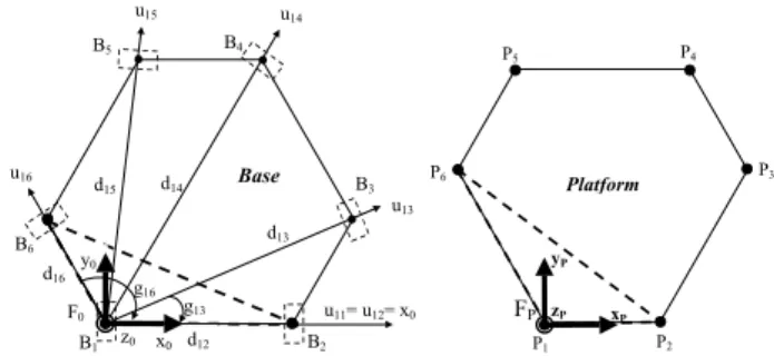
u11= u12= x0 z0 g16 g13 B2 F0 B1 B6 B5 B4 u16 u15 u14 u13 B3 d16 d14 d15 d13 d12 y0 x0 Base FP zP yP xP P1 P2 P6 P5 P4 P3 Platform

Fig. 2. Frame F0 fixed with the base and frame Fp fixed with the mobile platform.

(3)

respectively. The length of each leg is actuated using an active prismatic joint.

We define the frame F0 fixed with the base and the frame Fp

fixed with the mobile platform. To minimize the number of geometric parameters that are not equal to zero, we place these frames as follows (fig. 2) [15]:

- The origin of frame F0 is B1, the x0 axis is along B1B2 and

the (x0,y0) plane is defined by (B1,B2,B6).

- The origin of frame Fp is P1, the xp axis is along P1P2 and the

(xp,yp) plane is defined by (P1,P2,P6).

The axes of the first revolute joint of each leg are placed as shown in figure 2. The Khalil and Kleinfinger notations [16][17] are used to describe the geometry of the tree structure, which is composed of the base and the six legs. Each leg is composed of three moving links and three joints (2 passive revolute joints and 1 active prismatic joint).

Let ji denotes the link j of leg i, the local link frames are

defined as seen in (fig. 3). The geometric parameters defining these frames are given in table I, where a(j) denotes the antecedent of link j, the parameter µj is one for a motorized

joint and zero for a passive joint, σj = 0 for a revolute joint,

and σj = 1 for a prismatic joint. The parameters (γj, bj, αj, dj,

θj, rj) are used to determine the location of frame Fj with

respect to its antecedent Fi. It is denoted by the transformation

matrix [17]: 1         i i j j i j (1x3) R P T = 0 (1) Where: i j

R is the (3×3) rotation matrix :

i _{= }i i i _

j j j j

R s n a (2)

i j

P is the (3×1) position vector.

III. KINEMATIC MODELING

The following notations are used:

a3i unit vector along the z3i axis,

0 i

L represents the position vector P₁P_i referred to frame F0,

in the following the upper left exponent indicates the projection frame.

ˆ

0 i

L denotes the (3×3) skew symmetric matrix associated with

the vector 0 i

L .

0 p

V linear velocity of the origin of the platform P1.

0 p

ω angular velocity of the platform,

0 p

V linear acceleration of the origin of the platform,

0 p

ω angular acceleration of the platform,

0 P

V

(6x1) spatial velocity vector. It is composed of the

linear

and the angular velocities of the platform:

_{= } _   0 0 P P 0 P V ω V (3) 0 P

V The spatial acceleration vector:

_{= } _   0 0 P P 0 P V ω V (4) 0 pi

V linear velocity of point Pi of the platform:

0 =0 +0 ×0

Pi P P i

V V ω L (5)

0 pi

V linear acceleration of point Pi of the platform:

0 =0 +0 ×0 +0 ×

(

0 ×0

)

Pi P P i P P i

V V ω L ω ω L (6)

It can also be written as:

0 =_ −0ˆ _0 +0 ×

(

0 ×0

)

Pi 3 i P P P i

V I L V ω ω L (7)

Where I3 is the (3×3) identity matrix.

Γ (6×1) vector of the prismatic joint forces:

Γ= Γ

[

₃₁ Γ₃₆

T (11)

The following models are well-known [17][18] and will be used in the following:

i) The inverse kinematic model of the robot, which gives the velocities of the active joints q (i = 1 to 6) as a function of 3i the spatial velocity of the platform. It is defined by:

₌0 −1 0_V

a p p

q J (12)

The inverse Jacobian matrix of the robot is given as [18]:

Bi Pi q3i q2i q1i x3i z3i x0i z0i,x1i Li z2i z1i,x2i m3i=0 fi

Fig. 3. Link frames of a leg and reaction force fi between leg i and the

platform

TABLE I

GEOMETRIC PARAMETERS OF THE LEG i FRAMES

ji a(ji) µji σ ji γ ji b ji α ji d ji θ ji r ji

1i 0 0 0 γ1i b1i -π/2 d1i q1i 0

2i 1i 0 0 0 0 π/2 0 q2i 0

3i 2i 1 1 0 0 π/2 0 0 q3i

(4)

(

)

(

)

ˆ ˆ −       =_ _       T 0 T 0 0 31 1 31 0 1 p T 0 T 0 0 36 6 36 a L a J a L a (13) Where 0 3i

a is the unit vector along the z3i axis.

We recall that for a well designed parallel robot the matrix −

0 1

p

J should be regular in the reachable space [18], otherwise

the robot risk to be destroyed when approaching singularity. ii) The inverse kinematic model of a leg, which gives the joint velocities of the leg i (q₁_i,q₂_i,q₃_i) as a function of the linear velocity of point Pi: 0 1 0 i 3i pi q ₌ J− V ₍₁₄₎ 0 1 3i

J− _{is the inverse Jacobian matrix of leg i.}

The Jacobian matrix of the terminal point of leg i projected into frame F3i is obtained as:

( )

3i 3i 2i 0 q 0 q sin q 0 0 0 0 1     = −_ _     3i 3i J (15)

Its inverse is given as:

( )

(

3i 2i

)

3i 0 1/ q sin q 0 1/ q 0 0 0 0 1 −  −    =         3i 1 3i J (16) Note that: 0 −1₌3i −1 3i 3i 3i 0 J J R , 0 T 0 _i3i T 3i 3 3i J− ₌ R J− ₍₁₇₎ Where 0 −T 3i J denotes

(

0 −1

)

T 3i

J . This Jacobian is singular when

( )

2i

sin q = and/or 0 q3i= which are physically impossible. 0 iii) The second order inverse kinematic model of the leg i:

0 1

(

0 0

)

i 3i pi 3i

q ₌ J− V ₋ J q ₍₁₈₎

Substituting equation (7) into equation (18), we obtain:

= 0 -1

(

_ −0ˆ _0 +0 ×

(

0 ×0

)

−0

)

i 3i 3 i P P P i 3i i

q J I L V ω ω L J q (19)

IV. INVERSE DYNAMIC MODEL

The inverse dynamic model gives the motorized joint forces as a function of the position, velocity and acceleration of the

mobile platform. It is denoted by = 0 , 0 , 0

P P P

f ( T )

Γ V V .

Using the inverse geometric and kinematic models of the legs, we can compute the joint positions, velocities and accelerations of the legs

(

q_i,q_i,q_i

)

in terms of the platform trajectory. Since the platform and the legs are connected by spherical joints, then only pure reaction force fi exists between

leg i and the platform (fig. 3) [9][10].

The inverse dynamic model will be obtained by first computing f as a function of i Γ , by the use of the dynamic 3i model of leg i, then all the motorized joint forces Γ will be obtained from the Newton-Euler equations of the platform.

A. Computation of fi

The general form of the inverse dynamic model of a leg i, is written as [17]:

=

(

,

)

+0 T 0

i H q ,q qi i i i J3i fi

Γ (20)

Γi is the (3×1) vector of the torques/forces of leg i, where

Γ1i andΓ2i are zero, and Γ3i is the prismatic joint force.

Using equation (20) the reaction force can be written as:

0 _{= −}

(

,

)

₊0 −T i xi i i i 3i i f H q ,q q J Γ (21) Where: ₌0 −T

(

,

)

xi 3i i i i i H J H q ,q q (22) xi

H transforms H q ,q q from the joint space into the i

(

i i, i

)

position Cartesian space at point Pi [19][20].

Using equations (16) and (17) we obtain:

0 = −

(

,

)

+0 Γ_3i

i xi i i i 3i

f H q ,q q a (23)

B. Computation of the motor forces

The Newton-Euler equation of the platform is written as [17] [21][22]:

(

)

(

)

P M ˆ  _{ } _   = + _{− } _  _{ } _   0 0 0 P P P 3 0 0 0 0 P P P ₀ ₀ ₀ ₀ P P P P × × MS I g MS × I ω ω Ι ω ω F V (24) With: 0 p

F total external forces and moments on the platform about

the origin P1, 0g acceleration of gravity, I3 (3×3) identity

matrix, Mp mass of the platform,

0 p

I (3×3) inertia tensor of the platform with respect to frame F0, it is obtained by: 0 0 p 0 T p p p p I = R I R (25) p p

I (3×3) inertia tensor of the platform with respect to frame

Fp. It is written as: _PP P_P P_P P P P XX XY XZ XY YY YZ XZ YZ ZZ     =       P P I (26) 0 p

MS first moments of the platform:

P

[

MX MY MZ_P _P _P

]

T P MS = (27) 0 0 P P P P MS = R MS (28) 0 p

I (6×6) spatial inertia matrix of the platform [21]:

MP ˆ ˆ  −  =       0 3 P 0 p ₀ ₀ P P I MS MS I I (29)

The external forces and moments on the platform, which are due to the reaction forces of the legs are given by:

6 i 1= ˆ   =    

∑

F 3 0 0 p 0 i i I f L (30)

Substituting equation (23) into equation (30) and using (13) , we obtain [23]:

= 0 T

(

0 +0

)

p p leg

J

(5)

With: 6

(

)

i 1 , ˆ =    =        

ii) Calculate the Cartesian dynamic model of each leg Hxi.

iii) Calculate the forces and moments F , which represent the leg

forces and/or moments to overcome all Hxi.

iv) Find the forces and/or moments required to move the platform, F , as given by (24). P

)

(

)

(

)

ˆ   = − _ − _ − × × − − 0 0 xi xi 3 i P 0 0 0 0 xi P P i 3i i xi i i H A I L A ω ω L J q h q ,q V (34) Where: − − =0 T 0 1 xi 3i i 3i

A J A J is the (3×3) Cartesian inertia matrix of leg i referred at point Pi, andhxi 0J h3iT i

−

= is the Cartesain, Coriolis,

centrifugal and gravity forces of leg i at point Pi [19][20].

Substituting equation (34) into (32), and using (31) we obtain the direct dynamic model by:

0 = −0 −T + robot P p robot A V J Γ h (35) With: 6 P i 1 ˆ ˆ _M ˆ ˆ ˆ ˆ =  −   −    =  +   −         

∑

xi xi0 i 3 0 P robot ₀ ₀ ₀ ₀ ₀ P P i xi i xi i A A L I MS A MS I L A L A L (36)

(

)

(

)

(

)

(

)

(

)

(

)

6 i 1 P ˆ M ˆ =      =   × × − +        × ×  _ _   +_ _−   ×    

∑

3 0 0 0 0 robot 0 xi P P i 3i i xi i i i 0 0 0 P P P 3 0 0 0 0 P P P P I h A L J q h q ,q L MS I g MS I ω ω ω ω ω ω (37)

The symmetric and definite positive (6x6) matrix Arobot is

the total inertia matrix of the platform and the legs. The (6x1) vector hrobot is the total Coriolis, centrifugal and gravity

effects. The computation of the direct dynamic model is based, beside the calculation of the Jacobian matrices, on the

computation of Ai and hi of each leg. Many methods are

available to compute them [17][25][30]. To reduce the computational cost, customized symbolic methods and base inertial parameters can be used to obtain Ai and hi [26][31].

We note that:

i) Equation (35) represents the closed form solution of the

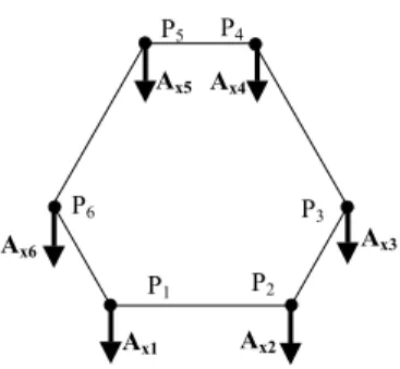
P1 P3 P2 P6 P5 P4 Ax6 Ax5 Ax1 Ax2 Ax4 Ax3

Fig. 5. Equivalent spatial inertia matrix of the legs.

P1 P3 P2 P6 P5 P4 -Hx6 -Hx5 -Hx1 -Hx2 -Hx4 -Hx3

(6)

direct dynamic model.

ii) The contribution of leg i on the inertia matrix of the robot

Arobot,is represented by the (3×3) mass matrix Axi located at Pi

(fig. 5). Each mass matrix Axi leads to the (6x6) symmetric

spatial matrix: ˆ ˆ ˆ ˆ  −  =    −    0 xi xi i xi ₀ ₀ ₀ i xi i xi i A A L L A L A L A (38)

ii) The mass matrix Axi induces a centrifugal force, which is

i xi P P i 3i i

L A ω ω L J q .

These terms are similar to the second term of the right hand side of the Newton-Euler equation of the platform (24). iii) The Coriolis, centrifugal and gravity forces of each leg are transformed into the (3×1) Cartesian force -hxi at point Pi.

VI. BASE INERTIAL PARAMETERS OF THE ROBOT

The dynamic models are obtained in terms of the inertial parameters of the links of the legs and of those of the platform. We use the following ten parameters for each link j: - XXj, XYj, XZj, YYj, YZj, ZZj: representing the six

independent elements of the inertia matrix around the origin of frame j (see equation (26));

- MXj, MYj, MZj: defining the first moments of link j;

- Mj: is the mass of link j.

The inverse dynamic model and energy model of the robot are linear with respect to these parameters [17][22][32], which we call standard inertial parameters. The base inertial parameters represent the minimum number of parameters from which the dynamic model can be calculated. The dynamic model complexity is reduced when computed by the base inertial parameters. Besides, they constitute the only identifiable parameters [22][26]. They can be obtained from the standard parameters of the links, by eliminating the parameters that have no effect on the dynamic model and by grouping some others.

A. Basic conditions for computing the base parameters

Since the kinetic energy and the potential energy are linear in the inertial parameters, thus:

10 m 10 m i i i i 1 i i 1 H H E U K h K K = = ∂ = + = = ∂

∑

(39) Where:

m is the number of the links. H is the total energy of the robot. E is the total kinetic energy of the robot.

U is the total potential energy of the robot.

Ki denotes an inertial parameter, hi is its coefficient in the

energy.

The expressions of the energy function for each inertial parameter are given in appendix A.

To determine the base inertial parameters, the following cases are considered [17][32], which can be deduced from the Lagrange equation:

1) An inertial parameter Ki has no effect on the dynamic

model, if its energy function is constant:

hi =constant (40)

In this case the parameter Ki is eliminated, it can be set as

zero.

2) An inertial parameter Ki can be grouped with some other

parameters Ki1,…,Kir if the energy function hi can be

expressed linearly in terms of the energy functions hi1, …, hir

[17][33]: i i1 i1 ir ir r ij ij j 1 h t h t h t h = = + +… =

∑

(41)

With tij is constant. The grouped parameters will be given as:

KijR =Kij+t Kij i j = 1 to r (42)

The index R indicates that some parameters are grouped with that one.

The base inertial parameters of the Gough-Stewart robot will be calculated by first determining the base inertial parameters of the legs, then the parameters of the platform will be taken into account.

B. Base inertial parameters of the legs

It has been shown that, if the Khalil and Kleinfinger notations are used to assign the link frames, then the base inertial parameters of a general tree structure can be completely determined using simple rules without computing the energy functions [17][33]. Concerning each leg of the Gough-Stewart robot, we can make use of the following three rules, which are applied recursively from the terminal link to the base:

Rule 1: If joint j is revolute, the parameters Mj, MZj and YYj

can be grouped with the parameters of links j and i, where i a( j)= is the link antecedent to link j. The grouping relations (when bj and γj are zero) are given in appendix B.

Rule 2: If joint j is prismatic, the parameters of the inertia matrix j_I

j can be grouped with the parameters of the inertia

matrix i_I

i with i = a(j), using the following relation:

i i i j j

iR i j j i

I = I + R I R (43)

Where j j

I is the inertia matrix of link j, it is the same as (26)

after replacing p by j.

This relation can be deduced from the fact that, in this case the rotational velocity of links i and j are the same. Relation (43) is developed in terms of the geometric parameters in appendix B.

Rule 3: If joint j is revolute and if a(j)=0, that is to say that link j is articulated on the base, then the parameters XXj, XYj,

XZj, YYj, YZj, MZj ,M j have no effect on the dynamic model.

This rule comes from the fact that, in this case, the x and y components of the rotational velocity of link j are zero and that the velocity of the origin of frame Fj is zero too.

Assuming general inertial parameters, there will be 30 standard inertial parameters for each leg i. Applying rule 2 on link 3i, the parameters XX3i, XY3i, XZ3i, YY3i, YZ3i, ZZ3i can

be grouped with the parameters of link 2 using the expressions given in appendix B. Then using rule 1 on link 2i, the

(7)

parameters YY2i, MZ2i and M2i can be grouped with the

parameter YY2i and with the parameters of link 1. This

recursive calculation ends with the application of rule 3 on link 1i to eliminate the parameters XX1i, XY1i, XZ1i, YY1i,

YZ1i, MZ1i, M1i. Thus, we have 14 base inertial parameters for

each leg. They are given by: ZZ1Ri, MX1i, MY1Ri, XX2Ri,

XY2Ri, XZ2Ri, YZ2Ri, ZZ2Ri, MX2i, MY2i, MX3i, MY3i, MZ3i,

M3i. The grouping relations are:

ZZ1Ri =YY2i+ZZ1i+ZZ3i (44) MY1Ri =MY1i−MZ2i (45) XX_2Ri =XX_2i+XX_3i−YY_2i−ZZ_3i (46) XY2Ri=XY2i−XZ3i (47) XZ2Ri =XY3i+XZ2i (48) YZ2Ri =YZ2i−YZ3i (49) ZZ_2Ri=YY_3i+ZZ_2i (50)

C. Base inertial parameters of the closed loop structure

More parameters could be eliminated or grouped when considering the closed structure (legs and platform). For this step we present a solution leading to determine them explicitly for a general Gough-Stewart structure. We note that for the legs, we grouped the inertial parameters of a link with its antecedent. For the platform we choose to group the parameters of the legs with those of the platform, such that the inertial parameters of the different legs remain identical.

Since the origin of the terminal frame of each leg (frames 3i) and the point Pi are the same thus:

V3i =VP+ωP×Li (51)

Applying relation (73), given in appendix A, the energy function of the mass M3i is obtained as:

M3i 1 h 2 = 3i T 3i 0 T 0 3i 3i i V V - g P (52) Since: 3i P =

(

P P P

)

3i Pi P p i V = V V + ω × L (53) and: 0 =

(

0 0 P

)

i p p i P P + R × L (54)

Equation (52) can be developed as follows:

(

)

(

)

(

)

P 2 P 2 P P

M3i 1,P 2,P 2,i 3,i 1,P 1,P 1,i 2,i

P 2 P 2 P P

3,P 3,P 1,i 2,i 2,P 3,P 2,i 3,i

P 2 P 2 P P

2,P 2,P 1,i 3,i 1,P 3,P 1,i 3,i

P P P

2,P 3,P 1,i 3,P 2,P 1,i 1,i

P P 3,P 1,P 2,i 1,P 3,P 2, 1 h L L L L 2 1 L L L L 2 1 L L L L 2 V L V L L V L V L = ω ω + − ω ω + ω ω + − ω ω + ω ω + − ω ω + ω − ω − + ω − ω 0 T 0 P g s P i 2,i P P P

1,P 2,P 3,i 2,P 1,P 3,i 3,i

L V L V L L 1 2 − + ω − ω − + − 0 T 0 P 0 T 0 P P T P 0 T 0 P P P g n g a V V g P (55) Where: = V1,P V2,P V3,PT P P V , ω = ω 1,P ω2,P ω3,PT P P , 0 _{= }0 0 0 _T P P P P R s n a , P P P T

1,i 2,i 3,i

L L L   =   P i L .

From equations (55) and equation (73), given in appendix A, we can deduce that the energy function of the parameters

M3i (i = 1 to 6) can be expressed in term of the energy

functions of the inertial parameters of the platform, such that:

(

)

(

)

(

)

P 2 P 2 P P

M3i 2,i 3,i XXP 1,i 2,i XYP

P P P 2 P 2

1,i 3,i XZP 1,i 3,i YYP

P P P 2 P 2

2,i 3,i YZP 1,i 2,i ZZP

P P P

MP 1,i MXP 2,i MYP 3,i MZP

h L L h L L h L L h L L h L L h L L h h L h L h L h = + − − + + − + + + + + + (56)

Thus, using (41) and (42), we can group the parameters M3i

with the inertial parameters of the platform. Taking into

account that P P P P P

1,1 2,1 3,1 1,2 3,2

L , L , L , L , L and P

3,6 L are zero, the grouped relations are:

6

{

(

P 2 P 2

}

RP P 2,i 3,i 3i i 3 YZ YZ L L M = = −

∑

(61) 6

{

(

P 2 P 2

}

5 P RP P 3,i 3i i 3 MZ MZ L M = = +

∑

(65) TABLE II

BASE PARAMETERS OF THE GOUGH-STEWART ROBOT Leg i (i = 1 to 6)

ZZ1Ri MX1i MY1Ri XX2Ri XY2Ri XZ2Ri YZ2Ri ZZ2Ri MX2i MY2i

MX3i MY3i MZ3i

Platform

XXRP XYRP XZP YYRP YZP ZZRP MXRP MYRP MZP MRP

TABLE III

ESSENTIAL PARAMETERS OF THE GOUGH-STEWART ROBOT Leg i (i = 1 to 6) ZZ1Ri XX2Ri ZZ2Ri MY2i MX3i MY3i MZ3i Platform XXRP XYRP XZP YYRP YZP ZZRP MXRP MYRP MZP MRP

(8)

_RP _P 6 _3i i 1

M M M

=

= +

∑

(66)

Physically, these grouped inertial parameters can be seen as the sum of those of the platform and the effect of masses M3i

suspended at points Pi for i = 1, …, 6.

Finally, we obtain 88 base inertial parameters for the Gough-Stewart robot (13 for each leg and 10 for the platform), they are summarized in table II, recall that the number of the standard inertial parameters is 190. The application of the QR numerical method to determine the base inertial parameters [17][34] validates this result.

Moreover, if we consider that the links are symmetrical and that the links 1 and 2 constitute one real link, then we can define the set of 52 essential parameters, given in table III.

VII. COMPUTATIONAL COST

The proposed algorithms of the dynamic modeling of the Gough-Stewart robot are implemented using customized symbolic technique and the base inertial parameters [22][31]. The numbers of operations to compute the different steps are given in [35]. The computation of the inverse dynamic model including the kinematic procedures of the legs needs 788 '+' and 1290 '*'. Where as the computation of the direct dynamic model needs 1120 '+' and 1823 '*'.

The comparison with the number of operations obtained by [10] and [11] is given in table IV. From the computational cost point of view, our method is equivalent to that of Gosselin [10], but we remind that our method can provide the inverse and the direct models and can be easily generalized for other structures.

Since the computation of the inverse dynamic model of the legs can be carried out in parallel, thus the proposed dynamic algorithms could be easily distributed on seven processors [11]. In this case, the computation cost of the inverse dynamic model is reduced to 226 '+' and 300 '*', and that of the direct dynamic model will be reduced to 387 '+' and 414 '*'.

VIII. CONCLUSION

In this paper, we highlight an interesting physical interpretation of the final form of the inverse and direct dynamic models of the Gough-Stewart robot. These models take into account all the dynamic parameters of the links. The approach is straightforward and could be applied to most parallel manipulators. These models are computed in terms of

the dynamic models of the legs. Consequently, the computation of these models can make use of the techniques, which were developed for the serial robots. To reduce the computation cost, the base inertial parameters of the robot have been determined analytically. Moreover, the computation of these models could be easily distributed on parallel processors. The numbers of operations of the inverse and the direct dynamic models are given.

APPENDIX A: EXPRESSIONS OF THE ENERGY FUNCTION hj

The total energy of link j is given as a linear relation in terms of the inertial parameters as follows [32]:

H_j =E_j+U_j j

j

= h K (67)

Where:

j

K is the (10×1) vector of the 10 standard inertial parameters;

The kinetic and the potential energy are computed by:

j

(

)

1 E M 2 2 × j T j j j T j j T j j j j j j j j j j j = ω I ω + V V + MS V ω (68) j j U 0 M     = −_ _       j j 0 T 0 j MS g T (69) 0 j

T is the transformation matrix of frame j relative to frame 0:

0 0 0 1   =     0 0 0 0 0 j j j j j s n a P T (70) j

h is the (1×10) vector defined by:

T j j j j j j j j H H H H XX XY MZ M  ∂ ∂ ∂ ∂  = _∂ _∂ _∂ _∂      j h (71) Thus:

hj= hXXjhXYjhXZjhYYjhYZ_jhZZjhMXjhMYjhMZjhMjT (72) Where: XXj 1, j 1, j 1 h 2 = ω ω ,hXYj= ω ω ,1, j 2, j hXZj= ω ω 1, j 3, j YYj 2, j 2, j 1 h 2 = ω ω ,hYZj= ω ω ,2, j 3, j ZZj 3, j 3, j 1 h 2 = ω ω hMXj= ω3, jV2, j− ω2, jV3, j− 0 T 0 j g s (73) hMYj= ω1, jV3, j− ω3, j 1, jV − 0 T 0 j g n h_MZj= ω_{2, j 1, j}V − ω_{1, j}V_{2, j}−0 T 0 j g a Mj 1 h 2 = j T j −0 T 0 j j j V V g P

APPENDIX B: GENERAL GROUPING RELATIONS

In the following we consider the special case where bj and γj

are zero. Two cases are considered:

1)If joint j is revolute, the parameters YYj, MZj and Mj can be

grouped with the parameter XXj and the parameters of the

antecedent link i using the following relations [32][33]:

jR j j XX =XX −YY 2 iR i j j j j j XX =XX +YY +2 r MZ +r M TABLE IV

COMPARISON OF THE NUMBER OF OPERATIONS OF THE INVERSE DYNAMICS Kinematic Modelling Inverse Dynamic Mod. Total Our method1 [35] 659 '*' and 299 '+' 631 '*' and 489 '+' 2078 Our method2 [35] 659 '*' and 299 '+' 715 '*' and 609 '+' 2282 Gosselin [10] 468 '*' and 282 '+' 834 '*' and 566 '+' 2150

Dasgupta [11] - - 4489

1_{using essential inertial parameters.} 2_{using base inertial parameters .}

(9)

iR i j j j j j j j XY =XY d S+ α MZ +d r Sα MZ iR i j j j j j j j XZ =XZ −d Cα MZ −d r Cα MZ

(

)

iR i j j j j j j j j j j j j j j j j XZ XZ CS S XX CC SS S XY C C XZ CS S YY S C YZ = + θ α + θ − θ α + θ α − θ α − θ α iR i j j j j j j j j j j j j j j j j j YY YY SS CC XX 2CS CC XY 2S CS XZ CC CC YY 2C CS YZ SS ZZ = + θ α + θ α − θ α + θ α − θ α + α (75)

(

)

(

)

iR i j j j j j j j j j j j j j j j j j j j YZ YZ SS CS XX 2 CS CS XY S CC SS XZ CC CS YY C CC SS YZ CS ZZ = + θ α + θ α + θ α − α + θ α + θ α − α − α iR i j j j j j j j j j j j j j j j j j ZZ ZZ SS SS XX 2 CS SS XY 2S CS XZ CC SS YY 2 C CS YZ CC ZZ = + θ α + θ α + θ α + θ α + θ α + α

Where: C(.) = cos(.), S(.) = sin(.), CC(.) = cos²(.), SS(.) = sin²(.) and CS(.) = cos(.) sin(.). The geometric parameters αj,

θj, rj and dj define frame link j with respect to frame i.

REFERENCES

[1] Nguyen C.C., Pooran F.J., "Dynamic analysis of a 6 d.o.f. CKCM robot end-effector for dual-arm telerobot systems", Robotics and Autonomous Systems, Vol. 5, pp.377-394, 1989.

[2] Ait-Ahmed M., "Contribution à la modélisation géométrique et dynamique des robots parallèles", Ph.D. Dissertation, LAAS, Toulouse, 1993.

[3] Bhattacharya S., Hatwal H., Ghosh A., "An on-line estimation scheme for generalized Stewart platform type parallel manipulators", Mechanism and Machine Theory, Vol. 32(1), pp.79-89, Jan. 1997.

[4] Bhattacharya S., Nenchev D.N., Uchiyama M., "A recursive formula for the inverse of the inertia matrix of a parallel manipulator", Mechanism and Machine Theory, Vol. 33(7), pp.957-964, Oct. 1998.

[5] Liu M-J., Li C-X., Li C-N., "Dynamics analysis of the Gough-Stewart platform manipulator", IEEE Transaction on Robotics and Automation, Vol. 16(1), pp.94-98, Feb. 2000.

[6] Codourey A., Burdet E., "A body oriented method for finding a linear form of the dynamic equatiojns of fully parallel robot", In IEEE Int. Conf. on Robotics and Automation, Albuquerque, New Mexico, U.S., 21-28 , pp.1612-1618, Apr. 1997.

[7] Tsai L-W, "Solving the inverse dynamics of a Stewart-Gough manipulator by the principle of virtual work", Journal of Mechanical design, March, Vol. 122, pp.3-9, 2000.

[8] Freeman R. A., Tesar D. "Dynamic modeling of serial and parallel mechanisms/robotic systems: Part I – Application, Part II - Methodology", Trends and Developments in Mechanisms, Machines and Robotics, Vol. 15(3), pp. 7-27, 1988.

[9] Reboulet C., Berthomieu T., "Dynamic models of a six degree of freedom parallel manipulators",In Proc. ICAR, Pisa, pp.1153-1157, , June 1991.

[10] Gosselin C. M., "Parallel computationnal algorithms for the kinematics and dynamics of parallel manipulators", IEEE Int. Conf. on Robotics and Automation, New York,Vol.(1), pp.883-889, 1993.

[11] Dasgupta B., Mruthyunjaya T.S., "A Newton-Euler formulation for the inverse dynamics of the Stewart platform manipulator", Mechanism and Machine Theory, Vol. 33(8), pp.1135-1152, Nov. 1998.

[12] Dasgupta B., Mruthyunjaya T.S., "Closed-form dynamic equations of the general Stewart platform through the Newton-Euler approach", Mechanism and Machine Theory, Vol. 33(7), pp.993-1012, Oct. 1998. [13] Dasgupta B., Choudhury P., "A general strategy based on the

Newton-Euler approach for the dynamic formulation of parallel manipulators", Mechanism and Machine Theory, Vol. 34(6), pp.801-824, Aug. 1999. [14] Ji Z., " Study of the effect of leg inertia in Stewart platform", In IEEE

Int. Conf. on Robotics and Automation, Atlanta, pp. 121-126, May 1993. [15] Zhuang H., "Self-calibration of a class of parallel mechanisms with a case study on Stewart platform", IEEE Trans. on Robotics and Automation, Vol. RA-13(3), pp. 387-397, 1997.

[16] Khalil W., Kleinfinger J.-F., "A new geometric notation for open and closed-loop robots", Proc. IEEE Conf. on Robotics and Automation, San Francisco, pp. 1174-1180, Apr. 1986.

[17] Khalil W., Dombre E., "Modeling, identification and control of robots", Hermès Penton, London, 2002.

[18] Merlet J.-P., Parallel robots, Dordrecht, The Netherland, Kluwer, 2000. [19] Khatib O., "A unified approach for motion and force control of robot

manipulators: the operational space formulation", IEEE J. of Robotics and Automation, Vol. RA-3(1), pp. 43-53, Feb. 1987.

[20] Lilly K.W., Orin D.E., "Efficient O(N) computation of the operational space inertia matrix", In proc. IEEE Int. Conf. on Robotics and Automation, Cincinnati, USA, pp. 1014-1019, May 1990.

[21] Featherstone R., "The calculation of robot dynamics using articulated-body inertias", The Int. Jour. of Robotics Research, Vol. 2(3), pp. 87-101, 1983.

[22] Khosla P.K., "Real-time control and identification of direct drive manipulators", Ph. D. Dissertation, Carnegie Mellon University, Pittsburgh, USA, 1986.

[23] Khalil, W, Guegan, S, "A novel solution for the dynamic modeling of Gough-Stewart manipulators", Proc. IEEE Int. Conf. on Robotics and Automation, Washington, DC, USA, pp. 817-822, May 2002.

[24] Luh J.Y.S., Walker M.W., Paul R.C.P., "On-line computational scheme for mechanical manipulators", Trans. of ASME, J. of Dynamic Systems, Measurement, and Control, Vol. 102(2), pp. 69-76, 1980.

[25] Megahed S., Renaud M., "Minimization of the computation time necessary for the dynamic control", In proc. 12th Int. Symp. on Industrial Robots, Paris, France, pp. 469-478, June 1982.

[26] Khalil W., Kleinfinger J.-F., "Minimum operations and minimum parameters of the dynamic model of tree structure robots", IEEE J. of Robotics and Automation, Vol. RA-3(6), pp. 517-526, Dec. 1987. [27] Guegan, S, Khalil, W, "Identification of the dynamic parameters of the

Orthoglide", In Proc. IEEE Int. Conf. on Robotics and Automation, Taipei Taiwan, pp. 3272-3277, Sep. 2003.

[28] Ibrahim O., Khalil W., Guegan S., "Dynamic modeling of some parallel robots", 35th_{International Symposium on Robotics, Villepinte, France,} 23-26 Mar., 2004.

[29] Craig J.J., "Introduction to robotics: mechanics and control", Addison Wesley Publishing Company, Reading, 1986.

[30] Walker M.W., Orin D.E., "Efficient dynamic computer simulation of robotics mechanism", Trans. of ASME, J. of Dynamic Systems, Measurement, and Control, Vol. 104, pp. 205-211, 1982.

[31] Khalil W., Creusot D., "SYMORO+: a system for the symbolic modelling of robots", Robotica, Vol. 15, pp. 153-161, 1997.

[32] Gautier M., Khalil W., "Direct calculation of minimum set of inertial parameters of serial robots", IEEE Trans. on Robotics and Automation, Vol. 6(3), pp. 368-373, 1990.

(10)

[33] Khalil W., Bennis F., "Symbolic calculation of the base inertial parameters of closed-loop robots", Int. Journal of Robotic Research, , Vol. 14(2), pp. 112-128, 1995.

[34] Gautier M., "Numerical calculation of the base inertial parameters", Journal of Robotic Systems, Vol. 8(4), pp. 485-506, 1991.

[35] Khalil W., Guegan S., "Efficient calculation of the inverse and direct dynamic models of Gough-Stewart Robots", Laboratory Report IRCCyN, Nantes, Jan. 2003.