Viscous flow and dynamic stall effects on vertical-axis wind turbines

(1)

Titre:

Title

: Viscous flow and dynamic stall effects on vertical-axis wind turbines

Auteurs:

Authors

: A. Allet et Ion Paraschivoiu

Date: 1995

Type:

Article de revue / Journal article

Référence:

Citation

:

Allet, A. & Paraschivoiu, I. (1995). Viscous flow and dynamic stall effects on vertical-axis wind turbines. International Journal of Rotating Machinery, 2(1), p. 1-14. doi:10.1155/s1023621x95000157

Document en libre accès dans PolyPublie

Open Access document in PolyPublie

URL de PolyPublie:

PolyPublie URL: https://publications.polymtl.ca/3668/

Version: Version officielle de l'éditeur / Published version_{Révisé par les pairs / Refereed} Conditions d’utilisation:

Terms of Use: CC BY

Document publié chez l’éditeur officiel

Document issued by the official publisher

Titre de la revue:

Journal Title: International Journal of Rotating Machinery (vol. 2, no 1)

Maison d’édition:

Publisher: Hindawi

URL officiel:

Official URL: https://doi.org/10.1155/s1023621x95000157

Mention légale:

Legal notice:

Ce fichier a été téléchargé à partir de PolyPublie, le dépôt institutionnel de Polytechnique Montréal

This file has been downloaded from PolyPublie, the institutional repository of Polytechnique Montréal

(2)

Reprints available directly from thepublisher

Photocopyingpermittedbylicenseonly Gordonand BreachScience PublishersPrinted inSingaporeSA

Viscous

Flow

and

Dynamic Stall Effects

on

Vertical-Axis Wind

Turbines

A. ALLET

and

I. PARASCHIVOIU

Departmentof Mechanical Engineering,

lcole

Polytechnique de Montr6al, C.E 6079, Succ. CentreVille, Montr6al, Qu6bec,

Canada, H3C 3A7

The presentpaperdescribes a numericalmethod, aimedtosimulatetheflow field ofvertical-axiswindturbines,basedon

thesolutionof thesteady,incompressible,laminar Navier-Stokesequations in cylindricalcoordinates.The flow equations,

written in conservationlawform,arediscretized usingacontrol volumeapproachon astaggeredgrid. The effect of the spinning bladesissimulatedbydistributingatime-averagedsource terms inthering of control volumes thatlieinthepath

of turbineblades. The numerical procedureused here, based on the control volume approach, is the widely known

"SIMPLER"algorithm. Theresultingalgebraicequationsaresolvedbythe TriDiagonal MatrixAlgorithm (TDMA)inthe

r-andz-directionsand theCyclicTDMAinthe 0-direction. The indicial modelisusedtosimulatetheeffect of dynamic stallatlow tip-speedratiovalues. The viscousmodel,developedhere,isusedtopredictaerodynamic loads andperformance

for theSandia 17-m windturbine.Predictions of theviscousmodelare comparedwithboth experimental data and results from theCARDAAVaerodynamic code basedontheDouble-MultipleStreamtubeModel. Accordingtothe experimental results, the analysis of local andglobalperformancepredictionsbythe3Dviscousmodel including dynamic stall effects showsagoodimprovementwithrespecttoprevious 2D models.

KeyWords: Wind turbines; Navier-Stokes;Dynamicstall;Aerodynamics;Finitevolume

indenergyisconsideredtobeapromising

renew-able energy source,particularlyforremote areas,

likeislandsand mountainous regions. Advances in

large-scale wind energy systems, significant cost reductions,

more efficient manufacturing techniques, increasing

technical experience and the increasing environmental awareness have contributed greatly to the use of wind

energy. Althoughinvented in 1931, the Darrieusturbine

did not see extensivedevelopmentuntilthe1970s during the world wideoilcrisiswhere a considerableamountof work has been done withregard tothe aerodynamics of vertical-axis wind turbines. Aerodynamic analysis of vertical-axis wind turbines isbased on several methods

which can be classified into two major categories:

momentummodels andvortexmodels.Updatedreviews

of the state of the art of such methods, including the appropriate references areprovidedbyStrickland[1986],

Turyan

etal. [1987], and Paraschivoiu [1988].

Themajorcontribution to theunsteady aerodynamics

of the Darrieus rotor is dynamic stall, which occurs at

lowtip-speedratios anditseffects haveasignificantrole

in drive-train calculation, generator sizing and overall systemdesign. Therefore, the abilitytopredict dynamic stallis of crucial importance foroptimizingtheDarrieus wind turbine. The theoretical methods of dynamic stall are still limited in their scope and prohibitively

expen-sive in term of computer CPU time. Although

Navier-Stokes solvers have been usedto simulatedynamic stall

(Shida etal. [1987], Daube etal. [1989], Tuncer etal.

[1990], and Visbal [1990]), most of the studies were

concerned with helicopterretreating-blade stall or agile

fighteraircraftand havethusconsideredpitchingairfoils

andnotthe rotationmotionencounteredbythe blades of

a Darrieus turbine. That is why our research group,

attachedto theJ.-A. BombardierAeronautical Chair, is

working on a Navier-Stokes solver able to simulate the

flow aroundanairfoil inDarrieusmotionunder dynamic stall conditions(Tclaonetal.[1993]). Ourresearchgroup

has also investigated several semi-empirical methods such as

Gormont,

MIT

and Indicial models (Allet and

(3)

Paraschivoiu [1988]). Forpractical reasons, the indicial model, which is one ofthe most recent semi-empirical

models, is used in this study to simulate the effects of

dynamic stall.

THREE-DIMENSIONAL

VISCOUS MODEL

Thesteady,incompressible,laminarNavier-Stokes

equa-tions in cylindrical coordinates are solved for the flow field and

_Performance

characteristics of a vertical-axis windturbine. This approach was firstdeveloped for the Euler equations (Rajagopalan [1985]) and extended to Navier-Stokesequations(Rajagopalan [1986]).Theflow

equations, written in conservation law form, are

dis-cretizedusingacontrolvolume approachandthe result-ing elliptic equations are solved by a line-by-line method. The numerical procedure used for solving the flow governing equationsis basedon the widely known

"SIMPLER" algorithm developed by Patankar [1980].

The turbinebladesaremodeledthroughthe sourceterms

inthemomentumequations usedtosolve the flowfield.

The essentials of this analysis are presented in the following subsections.

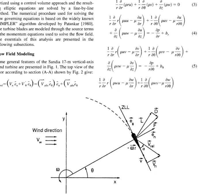
Flow FieldModeling

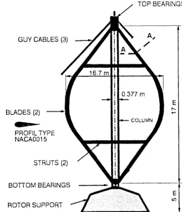
Some general features of the Sandia 17-m vertical-axis

windturbine arepresentedinFig. 1. The topviewof the

rotor according to section(A-A) shown by Fig.2 give:

0:

or)

(1)

where

V

(ucos

+

wsin)

V

(v-or)

(2)

Since or, the linear velocity of the turbine

_{blade_z}

is

known, theonlyunknowninthe above equationis

_Vabs.

Solutionof thevelocity fieldwouldyieldtheknowledge

of all the quantities ofinterest.

Withtheassumptionsstated previously, thegoverning

equations for the flow field of a vertical-axis wind

turbine are: 10

-

10 0

(pr)

+

(p)

+

(pw)

o

r Ouu-p

+-

puv-rOr

r-

P-O(

Ou)

Op

-+-

puw _lu

-

b

Oz

Or (4) r 9UV-lU

+-

9vv-

+

rOr

-r

r-

P-pvw l.t

-z

_rO0 (5) r _9wu p

+-

9wv-rOr

-r

r--d

Y-Wind direction

V

\x-ee

L

vo

x

(4)

TOPBEARINGS GUYCABLES

(3)

BLADES (2) PROFILTYPE NACA0015 0,377m COLUMN STRUTS

(2)

BOTTOMBEARINGS ROTORSUPPORT

FIGURE2 Angles,velocityvectorsand forces (sectionA-A).

+

9ww lU

-Z

_OZ

(6)

In the simulation of the incompressible flow, the basic equations aregenerallyexpressedasthe conservation of physical values such as mass or momentum. According

to the Finite Volume Method (FVM), the governing

equationsareintegratedovereach control volume cellto

derive the discretizedequations from them.For

velocity-pressure coupledflows, astaggeredgrid systemisknown

to give more realistic solutions and is adopted in the presentanalysis.

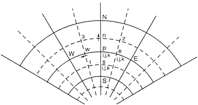
Computational Grid

The computational domain is subdivided into control

volumes by series of grid lines orthogonal to the

f’r,

0,

z

coordinate directions.The size of the control volumes is decidedbasedontheaccuracy requiredintheregion.

Patankar 1980] suggestedtouseastaggered gridforthe

storageof each variabletoavoid awavysolution and this

strategyisadoptedinthe presentstudy.

In

thestaggered

grid, the velocity components are calculated for the points thatlie onthe faces of the control volumes.Thus,

ther-directionvelocity uiscalculatedatthe faces thatare

normal to the r-direction.

It

is easy to see how the

locations for thevelocity components v and w aretobe

defined. Typical cells for each variable (u, v, w, p) are

shown onFigures 3 and 4.

TurbineModeling

The motion of vertical-axis wind turbine blades

intro-ducesprimarily a changein the localmomentumof the fluiddue to theforces generated by the rotating blades.

Thus, an obvious place to introduce the action of the

blades in the governing equations of the flow field is

through the source terms in the momentum equations,

namely

Sr,

_So

and

_Sz.

These sourcetermsare validonly

for the computational cells that lie in the path of the turbine blades. Following the detailed procedure illus-trated by Allet [1993], only the final form of the time-averaged sourceterms is given here:

S

WCOS(CDUCOS

_CLV

+

Czwsin)

(7)

S

W(CDV

+

_CLV

_CDtOr

(8)

(5)

W

e

\

1/

FIGURE3 Staggeredgrid(2-Dview).

p

cell

3

v cell

3

N

u

cell

w cell

(6)

These are forces feltby the blades perunit ofspan, and

are thus subtracted in the discretized momentum

equa-tions toeffectanequalbutoppositereaction onthe fluid

at a specificcell.

DYNAMIC STALL

ANALYSIS

Dynamic stall is an unsteady flow phenomenon which

referstothe stalling behavior of anairfoilwhentheangle

of attack is changing with time.

It

is characterized by

dynamic delayofstalltoangles significantly beyondthe

static stall angle and by massive recirculating regions moving downstream over the airfoil surface. Inthe case oftheDarrieusturbine, when theoperationalwindspeed

approaches itsmaximum, all blades sections exceed the

staticstallangle,theangleof attackchanges rapidly,and the whole blade works indynamicstall conditions.This

phenomenon maycausestructural fatigue, and even stall

flutter leading to catastrophic failure, and thus can

become, inmanycases, theprimarylimiting factor in the

performance and structure ofthe turbine. Therefore, in

orderto predict the aerodynamic performances of such

structures and provide aerodynamic loading information

tostructural dynamic codes, anumerical modelmustbe able to capture the complex aerodynamics encountered

by a vertical-axis rotor blade, andmore particularly the

dynamic stall phenomenon.

To provide some representation of dynamic stall

effects,thereareseveral methodswhich canbe classified

in two categories: the theoretical and semi-empirical

methods. Theoreticalmethods are attractive andaccurate

in studying local insight of the dynamic stall

phenom-enon (boundary layer evolution, pressure distribution)

evenifthe required computational resources are

prohibi-tive. Howeverfor practical cases, semi-empirical meth-odsare stillusedtosimulatedynamicstalleffects within engineeringaccuracy.

A

generalreview of somedynamic

stall prediction models is providedby Reddy and Kaza [1987].

IndicialModel

Themethodology ofsemi-empirical models often relies

onthe reduction and resynthesis ofaerodynamictestdata

from unsteady airfoil tests.

In

the interest of

computa-tional simplicity, some modelssacrificephysicalrealism and so may have limited generality in theirapplication.

The aim of this section is to introduce the indicial method used in our aerodynamic analysis to simulate dynamic stall. This model, originally developed by

Beddoes 1983, 1984] intheearly80’ s, has continuedto

improvesince then(BeddoesandLeishman[1989]).The

theoretical approach of the indicial method is quite

different from the other methods. The indicialmethodis

basedonthe fact thatdynamicstall is asuperpositionof distinct effects that may be studied separately by using indicialfunction(responseofasystemto adisturbance).

These effectsconsistsof three distinct parts: Potentialflow solution (linearsolution);

Separated flow solution for the non-linear airloads;

Deep

stall solution forvortex induced airloads.

This modelis thenrepresented by a relatively simple

set of equations and, most importantly, allows closer

identification ofthe interacting phenomena involved in

dynamic stall.

Potential

_flow

calculation.

Any

unsteady

aerody-namic model must be able to represent correctly the attached flow behavior. This flow induces two

aerody-namic components. The firstcomponent is acirculatory one

(CNc)

due to thechange in the angleof attack and has alagbehavior.

Cuc(t

_CIa

Ecosoe (10)

whereeE, the effective angleofattackis definedby:

with

OE--"On_

+

0 (t) (11)

c(t)

Ao-A

exp(-blS’

-A2

exp(-b2s’

(12)

Theconstantsof

Eq.

(12)aredeterminedonthe basis of theoretical considerations andoptimization tofit

experi-mental results (Beddoes [1984]), so the constants are given as

A

_o 1.0,

A

0.3,

A

2 0.7,

bl

0.35 and b2

0.68.

The second aerodynamic response is an impulsive

componentresulting fromaninducedvelocity normalto

the airfoilsurfacegenerated bythe airfoilmovementand

is given by: where

(4(t)AoO

CNI(

(13) M

el(t)

exp (14)

The normal force coefficient

_CN

resulting frompotential flow is obtainedby asimple summation:

(7)

CN(t

CNc(t

+ CNI(t

(15)

Thetangentialforce coefficient is givenby:

CT(t

CLa12

Esin12e

(16)

Non-linear

_effects.

Theunsteadynon-lineareffects are simulated through empirical correlations. Leading edge

and trailing edge separations must be predicted with

accuracy because oftheirgreat influenceon the

aerody-namiccoefficients.Tomodeltrailingedge separation,the

position of the separation point f is required. This

positionwillbe corrected later forunsteady cases.

f=

0.38

exp(12

12)/S

12<-12

(17)

f=

0.62

+

0.38(12

12)S

(exp(-1/S)- 1)

121<12

<--

_t22

(18)

f=

0.025

+

0.175

exp(122

c)/S

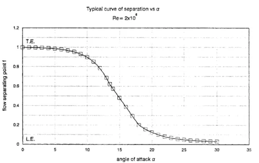
2 12>c2 (19)

A

typicalcurve of theseparation pointfvs.theangleof

attack12isshown inFig.5. Theparameters_121,_o2,

S,

$2,

$3 arefound from the curve-fitting of the static lift and

drag curves. The non-linear value of the normal force coefficient is determinedby"

CN

N-L

+

f0.5)2

Cu

C (20)

For unsteadyflows, temporaleffects influence the

posi-tion of the separation point. Two first order lags are therefore introduced to take these effects into account.

The first function simulates the airfoilunsteadypressure response.

C

N,

+p(t)

CNN_

L

(21)

where

qbp

(t)

1-exp

cTp

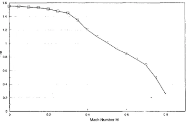
(22)

The onset of leading edge separation is related to the following criterion:

CN,

>

_CN1

with

_CN1

beingthe critical normal force coefficient illustrated in Fig. 6.

A

second

linear lag function is introduced to simulate additional effects of the unsteady boundary layer response:

CNF,

dPF(t

CN,

(23)

where

(

,--2Vt

+F

(t)

1--exp

CTF

]

(24)

A

new angleof _{attack, 12F is defined from the value of}

CNF,"

CNF’

₍₂₅₎

12F--

_CLot

1.2

Typical curveof separationvs z

06

Re 2xl

10 15 20 25 30

angleofattack(]

FIGURE5 Typicalcurveof the position of the flowseparation pointfunction ofo.

(8)

4Mach

FIGURE 6 Critical normal force coefficient(CN1) for theonset of

leadingedgeseparationfunctionof the Mach number.

Thisangleisusedinsteadofotin

Eqs.

17-19tocompute

theposition of the unsteady separation.

Deep

dynamic stall. Formost dynamic stall cases, a vortex appears nearthe leading edge and moves

down-stream on the upper surface of the airfoil. Until the detachment of thevortex, it seemsthereis nosignificant

change in the airfoil pressure distribution. Thus, the

inducedvortex liftcontributionisequaltothe loss of lift

due to the separation (Fig. 7)

where

C_v

_CNC

(1 -K)

(26)

K

(1

+f0.

)2

(27)

4

From experimental observation, ithas been proven that

the reattachment of the unsteady flow occurs later relatively tothesteadycase. Thisdelayisintroducedby

angleofattack

FIGURE7 Dynamic stallvortex contribution.

replacing o from eqs. 17-19 by a modified angle

_o

givenby:

(28)

RESULTS

AND

DISCUSSION

This section presents a selection of results obtained by

both the three-dimensional viscous model developed

previously and theCARDAAVcode basedonstreamtube

theory.Thecorrespondingresultsarecomparedwiththe

experimental data on the Sandia 17-m wind turbine

configuration provided by Akins [1989]. The dynamic

stall is simulated bythe indicial model for both

aerody-namiccodes. First,tovalidatetheviscouscode, prelimi-narytests dealing with the determination of the

compu-tationalgridandtheconvergenceof the numerical model

are presented.

Computational Mesh and

Convergence

Considerations

Tovalidate this solver, preliminary results forvalidating

thecomputational procedurearepresented.Thus, for the

windturbineproblem, it was necessary to firstestablish thesizeof thecomputationaldomain whichisreferredto asthe worldsize.Thedomainwas consideredtobelarge

or accurate enough when the power coefficient reached

anasymptoticvalue.Thisexercisewascarriedoutonthe

Sandia 17-m wind turbine rotating at 42.2rpm and a

tip-speedratio

Xeq

6.12.Thisvaluewasused instead of otherexperimentalvaluestoavoid the effects ofdynamic

stallphenomenaon thecomputedresults.

As

shown inFig. 8, thepowercoefficient

Cp

reached

itsasymptoticvalueat aworldsize of about

60Req.

The

sameexercisewascarriedoutforthe0-gridsizewhichis

illustratedbyFig. 9. Accordingtothisfigure,a minimum

of 40pointsareneededtogeta sufficientcomputational

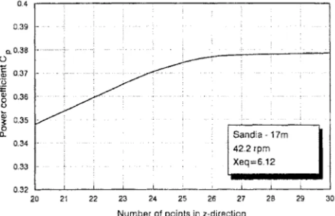
grid in the 0-direction.Forthe z-direction, Fig. 10 shows that 26 points at least were necessary to getan

asymp-totic value of

_Cp.

Thus, for all the following computa-tions, the fineness of the gridwas maintained at

(66

48 26) points. Alastfeature about Fig. 10isthatatthe

end of theoptimizationexercise, the calculated value of

the power coefficient

Cp

is almost equal to the

corre-sponding experimentalvalue

(Cp(exp)

0.387).

A

conver-gence history of

_Cp

with the number of iterations is

presentedinFig. 11 for the same conditions used in the

determination of the grid size.As seen in this figure, a

(9)

0.4 0.39 L)

"

0.38 0.37

o

0.36 0.35 0.34 Sandia

-17m

42.2rpm | FIGURE 8 20 40 60 80 100

Worldsizein diameters

Effect of worldsize in r-directiononpowercoefficient.

and even before that.

In

general, the calculations were taken to250iterations toassuretheconvergence behav-ior of the computed solution for different operational

regimes of the Darrieus wind turbine. Following this

optimization exercise, the resulting computational mesh

(66 48 26) usedbytheviscoussolveris shownby

Fig. 12.

LocalAerodynamic Coefficients

The distribution oflocal normal force coefficient C_N at

the equator levelis plotted asa function of the azimuth

angle to for values oftip-speedratio

Xeq

varying from

2.33to4.60.fortheSandia 17-mwind turbinerotatingat

38.7rpm according to the experimental data (see Figs.

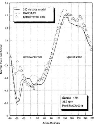
13-15). Figure 13 shows that theviscous model

repre-sentsquiteaccuratelythe distribution ofthe normalforce

coefficientfor almost all azimuthanglevalues.

However,

near 0 -60 deg. in the downwind zone, predictions

aredifferent fromexperimental data.Akins 1989],in his

experimentaldata analysis, hascomparedthe

experimen-tal data to values predicted by a vortex model coupled

withGormont model(as dynamic stall model) as

modi-fied by Mass6 [1981]. Akins concluded in his analysis

0.4 0.39 0.34 _42.2_rpm 0.33 Xeq=6.12 0.32 20 21 22 23 24 25 26 27 28 29 30 0.38 0.37 0.36 0.35

Number of points inz-direction

FIGURE10 Effect of gridpointsinz-direction onpowercoefficient.

thatthe wake interaction in thedownwind zone doesn’t allow the establishment ofdynamic stall.

However

this effect is not predicted by the vortex model (used by

Akins in his analysis) nor by the viscous model. In

general, values predicted by CARDAAV code are in

good agreement with experimental data even if the

maximum value in the upwind partis slightly overesti-mated. With increasing tip-speedratio

_(Xeq

3.09 and

4.60), this feature (wake interaction) tends to disappear

and the values predictedbyboth modelsagree quitewell with the corresponding experimental data.

This firstcomparison of the normal force coefficient

tendstodemonstrateacertain superiority of the indicial modelas adynamic stall model whencomparedtoother semi-empirical models (Gormont model for instance). Thus, CARDAAV code coupled with Gormont model

predicted a maximum value of

CN

in the upwind part

much greater than thecorresponding experimentalvalue

CNmax

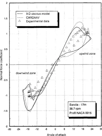
1.6 (Allet and Paraschivoiu [1988]). To better

visualize the dynamic stall phenomenacharacterizedby

anhysteresislooponnormal force coefficient

Cy

curves

vs. angle of attack o, Fig. 16 presents the variation of

0.45 0.4

0.35

0.25

20 25 30 35 40 45 50 55 60

Number of pointsinG-direction

FIGURE 9 Effect of grid points in 0-directiononpowercoefficient.

0.8 0,4 42.2rpm 0.2 50 100 150 200 250 300 Number of iterations

(10)

(a) (b)

FIGURE 12 Computational meshatthe equator in and 0 directions.

normal force coefficient vs the angle of attack for a

tip-speed ratio

Xeq

2.49 predictedbybothmodels. This figure shows that for both models dynamic stall does

exist in the upwind part (hysteresis loop) and that the reattachment of the boundary layer does happen at the

same time forboth models.

The values of local tangential force coefficient

Cw

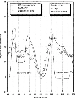
predictedby both aerodynamic codes are presentedasa functionofthe azimuthanglein Figs.(17-19).Generally

speaking, the viscous code reproduces quite well the

1.6 1.2 0.8 0.4

"-

-0.4 E Z -0.8 3-Dviscousmodel CARDAAV Experimental data IIII downwindzone -1.2 -1.6 -2 -90 -60 -30 30 upwind zone Sandia 17m 38.7rpm ProfilNACA0015 60 90 120 150 180 210 240 270 Azimuthangle

FIGURE 13 Normal forcecoefficient vs. azimuthangleat38.7rpm

and_Xeq=2.33.

3-Dviscousmodel

CARDAAV Experimentaldata

downwindzone upwind zone

Sandia 17m 38.7rpm

ProfilNACA0015

30 60 90 120 150 180 210 240 270

Azimuthangle

FIGURE 14 Normal forcecoefficient vs. azimuthangleat38.7rpm

andXeq 3.09.

experimentalvalues of the tangential force coefficient

_Cw

except near0 30 deg. in the upwind zone where the

predictedvalues areslightlyoverestimated.Theonsetof

dynamic stall tends to give a kind of irregularityto the

curves of the tangential force coefficient which tends to

disappear with increasing tip-speed ratio (Figs. 18 and

19). CARDAAV predictionsof

Ca-

areingeneralingood

agreement with experimental data, though the part de-finedby 150 deg. < 0 deg. inthe upwindzonepresents

predictions completelydifferent from the corresponding

experimental data. Moreover, for almost all cases

pre-sented, this model overestimates the maximum value of

thetangentialforcecoefficientin theupwindand

down-windzones of the Darrieus windturbine.

Global Performance

Theevaluationof thepowercoefficient

_Cp

wascomputed

on the Sandia 17-m wind turbine operating at 42.2 and

50.6rpm. Evenif theeffect ofdynamicstallis notreally

visibleonpowercoefficientcurves, however thiskindof curves allows one to have a better idea about the

(11)

1.2 0.8 0.4 -0.4 -0.8 -1.2 3-Dviscousmodel

/

,--,,

Experimentaldata

I

.5 CARDV

i

’’"’""’’

’/

x.er,e,a,.a,a

!.

o.

",i,

Jownwindzone

!

/

upwindll

izone

.7rp

_I

ProfilNACA0015

-90 -60 -30 30 60 90 120 150 180 210 240 270

Azimuthangle

upwind zone

FIGURE15 Normal forcecoefficient vs. azimuthangleat38.7rpm

and_Xeq 4.60. Z-0.5 -1.5 downwindzone 17m 38.7rpm ProfilNACA0015 -2 -30 .24 .18 .12 .6 12 18 24 30 Angleofattack

FIGURE16 Normalforcecoefficient vs.angleofattackat38.7rpm

and_Xeq 2.49.

powercurvesdealwithgreaterwindvelocities. Predicted and experimental values of thepower coefficient

_Cp

vs.

tip speed ratio

Xeq

arecomparedin Figs. 20 and 21. In

the dynamic stallzone(1 <

Xeq

<4), both models seem

to reproduce quite accurately this zone however in the

transition zone(4<

Xeq

<6),both modelsunderestimate

the maximum value of the power coefficient. For the unstalledregion,it isobviousthat the viscous codeoffers betterpredictions than CARDAAV code.Figure21 was

reproducedmainly from the reference of

Touryan

etal.

[1987] for a rotational speed of 50.6rpm. This figure

offers a more interesting comparison between several aerodynamic models and the viscous code. These aero-dynamic codes are: double-multiple streamtube model

(CARDAAV, CARDAAX)of Paraschivoiu [1988], the

model basedon vortextheory (VDART3) developed by

Strickland _[1979] and the modelbasedon local

circula-tiontheory (MCL) developedbyMass6[1986].First, we

have to notice that this figure shows results of two versions ofthe CARDAAV code: oneusing the indicial model and the other using

Gormont

model as dynamic

stallmodel.

Moreover,

the secondversionofCARDAAV

takes intoaccountsecondaryeffects whichareimportant

at high tip-speedratio values. Consequently, differences are noticedbetween predicted results of bothversionsof

CARDAAV.

In

the dynamic stall regime

(Xeq

< 4), the

coupling CARDAAV/Indicial code seems to give better

results than CARDAAV/Gormont code. According to

experimental data, the viscous model provides a good

representation ofthe power coefficient in all ranges of

tip-speedratio

Xeq

evenifthe Local Circulationmethod

seems to bethe best model that reproduces quite

accu-rately the distribution of theperformance coefficient C_P

in almost alloperational ranges of

_Xeq.

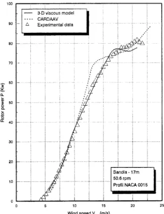
The dynamic stall phenomenon is clearly visible on

thepowercurvescharacterizedbyaplateauathighspeed

(Figs. 22 and

23).

Comparison of rotor power values predicted by both models and experimental data is

presentedinFigures 22 and 23. Forlow wind velocities

(Veq

< 10m/s), both models seem to give a good

approximationof the experimental values ofrotorpower,

thoughin thedynamic stall regime

(Veq

> 12.5m/s),the

CARDAAV code using the indicial model does not

predictanalmostconstantvalue andkeepsonincreasing.

The viscous model predicts a plateau close to the

(12)

3-Dviscous model Sandia-17m CARDAAV 38.7rpm

,

Experimentadata ProfilNACA0015

3-D viscousmodel

/

Sandia 17m

CARDAAV

I

38.7rpm

A _Experimental_data _Profil_NACA₀₀₁₅

0.4 -..7;;i

.90 -60 -30 30 60 90 120 150 180, 210 240 270

AzimuthAngle

FIGURE 17 Tangential forcecoefficient vs. azimuth angle at 38.7

rpm and_Xeq 2.33. 0.5 CARDAAV 38.7rpm /k _Experimental_data ProfilNACA0015 3l A

:

i

’ ;.>;:;

-90 -60 -30 30 60 90 120 150 180 210 240 270 Azimuthangle

FIGURE 18 Tangential force coefficient vs. azimuth angle at 38.7

rpm andXeq 3.09.

-90 -60 -30 30 60 90 120 150 180 210 240 270

Azimuthangle

FIGURE 19 Tangential force coefficient vs. azimuth angleat 38.7

rpmand_Xq 3.70. 3-D viscous model CARDAAV

_I

L Experimentaldata

I

) 0.3 .u_ 0,1 10 Tip-speedratioXq

FIGURE20 Powercoefficientvs.tip-speedratioforSandia-17m at

(13)

PARASCHIVOIU 0 0.3

._

0.2

Sadia-

17m 50.6rpm

I

ProfilNACA0015

I

..."/ .m 3-D viscousmodel CARDAAV/INDICIAL CARDAAV/GORMONT CARDAAX VDART3 MCL / Experimentaldata 10 Tip-speedratioX_eq

FIGURE 21 Powercoefficient vs.tip-speedratioforSandia-17m at

50.6 rpm. 6O I:E ₄₀ lO0 CARDAAV 90 /k 3-Dviscousmodel Experimentaldata Sandia 17m 50.6rpm ProfilNACA0015 lO 15 20 25

Windspeed

Veq

(m/s)

FIGURE23 Rotor powervs.windspeedforSandia17mat50.6 rpm.

3-D viscousmodel

i

CARDAAV /x _Experimental_data 60 /.

""

/,,, o 20

’"i

Sandia-Tm .2rpm

,,’

ProfilNACA0015

1

10 15 20 25 Windspeed V_eq(m/s)

FIGURE22 Rotorpowervs.windspeedforSandia17mat42.2rpm.

However,

for a rotational speed of 50.6 rpm, Fig. 23 shows that predicted values of the powerare

underesti-mated in thedynamicstallregimeeveniftheplateaustill exists.

CONCLUSION

The main objective of this study was todevelop a new

computational procedure to analyze the global

perfor-mance and blade loads of vertical-axis wind turbines. This has been accomplished with a numerical solver based on the solution of the steady, incompressible,

laminar Navier-Stokes equations using Finite Vol-ume Method (FVM). Dynamic stall effects were

simu-lated by an indicial model (as dynamic stall model)

which tackles this problem at a more physical level of approximation but still in asufficiently simple manner.

Analysis of the computed results presented in the

previoussection has demonstrated certainsuccessof the

viscous solvercoupledwiththe indicial model regarding

its ability toaccuratelypredict the aerodynamic

(14)

support the factthat, among othersemi-empirical

mod-els, the indicial model offers the best representation of dynamic stall for theprediction ofwindturbine

perfor-mance.

As

afollow-up, considerableimprovementcould also

be achieved for future predictions.

For

instance this

numericalsolver could be easily extendedtoincludethe turbulentnatureof thewindbyusing a stochastic model

(see reference ofBrahimi and Paraschivoiu

[1992]).

Nomenclature c

c,

CN

CT

f n,O,s N P r,O,Z R Req S S,So,

_S

TSR

,

V,W bladechord,m

dragcoefficientof bladeairfoil section lift coefficientof bladeairfoilsection liftstaticcurveslope

normalforce coefficient of blade airfoil section power coefficient of theturbine

tangential force coefficient of blade airfoil

section

flowseparationpoint(%c)

bladelength,m

Mach number

coordinatesystem attachedtothe blade numberofblades

staticpressure, Pa

cylindricalcoordinatesystemattached’tothe blade

rotorradius at acertainlevel,m rotor radius atthe equator, m nondimensionaltime(t(1-M2)2V/c) rotorswept area, m

source termsin themomentumequations

time,

Tip-SpeedRatio(toReq/U)

velocity componentsinther,to,zdirections,

m/s

absolutevelocityofthe wind,m/s

component of_Vab.in then-direction,rn/s relativevelocity,rn/s

freestream wind velocity,m/s

time averaging factor(NCpVrelA0/4’rr)

tipspeedratio atthe equator(toReq/U)

local angle of attack, deg.

staticstall angle,deg.

local normalangle, deg.

dynamic stall reattachment factor,deg.

azimuthalangle,deg.

dynamicviscosity,Pa.s

cinematic viscosity,m2/s

density,Kg/m

rotorsolidity(NcL/S)

indicial function

rotorrotationalspeed,

s-Superscriptsand Subscripts

CIR,C circulatorycomponent

IMP,I impulsivecomponent

N-L non-linearcomponent

n-1 previoustimevalues

V vortexcomponent

eq equatorial values

freestream conditions

References

Akins,R.E., 1989.Measurementsof SurfacePressureon anOperating Vertical-Axis WindTurbine,ContractorReportSAND89-7051,

San-dia NationalLaboratories,Albuquerque,NewMexico87185. Allet, A. and Paraschivoiu, I., 1988. Aerodynamic Analysis of the

Darrieus Wind Turbines Including Dynamic-Stall Effects, AIAA

Journal_ofPropulsion andPower,Vol.4,no.5, pp. 472-477. Allet,A., 1993. Mod61e visqueuxtridimensionnelpour le calcul des

turbines axe vertical,Thgsededoctorat, D6partementdeG6enie

M6canique,lcolePolytechnique de Montr6al.

Beddoes,T.S.,1983. Representation ofAirfoilBehaviour,Vertica,Vol. 7,no.9, pp. 183-197.

Beddoes,T.S., 1984. PracticalComputationofUnsteadyLift, Vertica,

Vol.8,no. 1,pp.55-71.

Beddoes,T.S.,andLeishman,J.G.,1989.ASemi-Empirical Model for Dynamic Stall, Journal_oftheAmericanHelicopter Society, Vol. 34,

no.3, pp. 3-17.

Brahimi,M.T., and Paraschivoiu, I., 1992. Stochastic Aerodynamic Model for StudyingDarrieus Rotorin TurbulentWind, The Third

International SymposiumonTransportPhenomena and Dynamics_of Rotating Machinery,(ISROMAC-3),Hemisphere Publishing

Corpo-ration,pp. 463-477.

Daube, O., TaPhuoc,L.,Dulieu,A., Coutanceau, M., Ohmi,K.and Textier,A., 1989.Numerical SimulationandHydrodynamic

Visual-izationof TransientViscousFlow Around and OscillatingAerofoil,

International Journal_forNumericalMethods in Fluids,Vol. 9, pp. 891-920.

Mass6,B., 1981. Description de deauxprogrammesd’ordinateurpour

lecalcul de performancesetdes charges a6rodynamiquespour les 6oliennesaaxevertical,RapportIREQ-2379,InstitutdeRecherche

d’hydro-Qu6bec, Varennes,Canada.

Mass6,B.,1986.ALocal CirculationModel forDarrieusVertical-Axis

WindTurbine,JournalofPropulsion andPower,Vol. 2,no.2,pp.

135-141.

Paraschivoiu,I., 1988. Double-Multiple Streamtube Model for

Study-ing Vertical-AxisWindTurbines, AIAAJournalofPropulsion and

Power,Vol.4,no.4,pp.370-378.

Patankar,S.V., 1980.NumericalHeatTransferandFluidFlow,New

York: HemispherePublishingCorp.,McGraw-Hill.

Rajagopalan, R.G., 1985. Finite Difference Model forVertical-Axis

WindTurbine,Journal_ofPropulsion andPower,Vol. 1,no.6,pp.

432-436.

Rajagopalan, R.G., 1986. ViscousFlow FieldAnalysis ofa

Vertical-Axis Wind Turbine, Proceedings ofthe 2P’ lntersociety Energy

Conversion Engineering Conference, San Diego, Vol. 2, pp. 1242-1247.

Reddy, T.S.R.,andKaza,K.R.V.,1987.A Comparative StudyofSome

Dynamic Stall Models,NASATM-88917.

Shida,Y.,Kuwahara,K., Ono, K.,andTakami,H.,1987. Computation of Dynamic Stall ofaNACA-0012 Airfoil,AIAAJournal, Vol. 25,no.

3,pp.408-4 13.

Strickland,J.H.,Webster,B.T.,andNguyen,T.,1979.A VortexModel of the Darrieus Turbine: An Analytical and Experimental Study, JournalofFluids Engineering, Vol. 101,pp.500-505.

Strickland,J.H.,1986.AReview ofAerodynamic Analysis Method for Vertical-Axis Wind Turbines, Proceeding _ofthe 5’h _ASME _Wind

(15)

Tchon,K.-E,Allet,A.,andHall6,S.,1993. Dynamic StallSimulation

foraRotating Blade, Proceedings_oftheFirstBombardier

Interna-tionalWorkshop,Montr6al, Canada,pp.440-443.

Tuncer, I.H., Wu, J.C., and Wang, C.M., 1990. Theoretical and

Numerical Studiesof OscillatingAirfoils,AIAAJournal, Vol.28,no.

9,pp. 1615-1624.

Turyan,K.J., Strickland, J.H.,andBerg, D.E., 1987. ElectricPower

fromVertical-Axis Wind Turbines,A1AA Journal_ofPropulsion and

Power,Vol.3,no.6, pp. 481-493.

Visbal,M.R.,1990. Dynamic Stall ofaConstant-RatePitching Airfoil,

(16)

Internatfional Journal of

A

e

ro

spa

c

e

Eng

fin

e

r

fing

Hfindawfi Publfishfing Corporatfion

http://www.hfindawfi.com Volume 2010

Robo

Journal o

t

fics

f

H findawfi Publfishfing Corporatfion

Actfive and Passfive

Electronfic Components

Control Scfience and Engfineerfing

Journal of

http://www.hfindawfi.com Volume 2014 H

findawfi Publfishfing Corporatfion

findawfi Publfishfing Corporatfion http://www.hfindawfi.com

Journal of

En

g

fin

e

er

fin

g

Volume 2014

Subm

fi

t

your

manuscr

fip

ts

a

t

h

t

tp

:

/

/www

.h

findaw

fi

.com

VLSI Desfign

Shock and Vfibratfion

C

Advances

fiv

fi

l

Eng

fin

finee

r

fing

AcousAdvancestficsfin and Vfibratfion

Electrfical and Computer Engfineerfing

Journal of

Advancesfin

OptoElectronfics

The

Sc

fient

fific

Wor

ld

Journa

l

Senso

JouHfindawfi Publrnafishfing Corporatl ofionf

rs

Modellfing & Sfimulatfion fin Engfineerfing

Chemfical Engfineerfing

InternatfionalJournal of Antennas and Propagatfion InternatfionalJournal of

http://www.hfindawfi.com Volume 2014 H findawfi Publfishfing Corporatfion

Navfigatfion and Observatfion InternatfionalJournal of

Dfistrfibuted

Sensor Networks