HAL Id: hal-01459206
https://hal.archives-ouvertes.fr/hal-01459206
Preprint submitted on 7 Feb 2017
HAL is a multi-disciplinary open access
archive for the deposit and dissemination of
sci-entific research documents, whether they are
pub-lished or not. The documents may come from
teaching and research institutions in France or
abroad, or from public or private research centers.
L’archive ouverte pluridisciplinaire HAL, est
destinée au dépôt et à la diffusion de documents
scientifiques de niveau recherche, publiés ou non,
émanant des établissements d’enseignement et de
recherche français ou étrangers, des laboratoires
publics ou privés.
Parameterized complexity and approximability of
coverability problems in weighted Petri nets
Dimitri Watel, Marc-Antoine Weisser, Dominique Barth
To cite this version:
Dimitri Watel, Marc-Antoine Weisser, Dominique Barth. Parameterized complexity and
approxima-bility of coveraapproxima-bility problems in weighted Petri nets. 2017. �hal-01459206�
Parameterized complexity and approximability
of coverability problems in weighted Petri nets
Dimitri Watel1, Marc-Antoine Weisser2, and Dominique Barth3
1
SAMOVAR, Evry, France
2
LRI, CentraleSup´elec, Universit´e Paris-Saclay, Orsay, France
3 DAVID, Universit´e Versailles Saint-Quentin-en-Yvelines, Versailles, France This paper is submitted as a Regular paper.
Abstract. Many databases have been filled with the chemical reactions found in scientific publications and the information associated with (ef-ficiency, chemical products involved. . . ). They can be used to define functions representing costs such as the ecoligical impact of the reac-tions. A major challenge is to use computer driven optimization in order to improve synthesis process. The objective is to provide algorithms to help determining a pathway (series of reactions) for the synthesis of a molecule. Usually, a chemist proposes a pathway adapted from an exist-ing one. Our goal is to determine optimum pathways from the reactions recorded in the database.
As, the classical Petri nets do not allows us to consider the optimization component, a weighted model has to be defined and the complexity of the associated problems studied. In this paper we introduce the weighted Petri nets in which each transition is associated with a weight. We define the Minimum Weight Synthesis Problem: find a minimum weight series of transitions to fire to produce a given target component. It mainly differ from classical coverability as it is an optimization problem. We prove that this problem is decidable but EXPSPACE-hard and that there is no polynomial approximation even when both in and outdegree are fixed to two and the target state is a single component. We also consider a more constraint version of the problem limiting the number of fired transitions. We prove this problem falls into PSPACE and the parametrized versions into XP but it remains not approximable. Keywords: Petri net coverability problem, Minimum weight synthesis problem, Parameterized complexity, Approximability
1
Introduction
The development of decision support tools for the synthesis of new molecules is a major challenge for organic chemistry and biochemistry [7,17], through the use of databases of reactions that are regularly updated in these scientific fields (such as REAXYS, CHEBI [1,13]). Indeed, the objective is to provide algo-rithms to help determining a reaction pathway (serie of consecutive reactions) for the synthesis of new molecules by using such reaction databases [7,9]. Usu-ally, a chemist proposes a reaction pathway from a synthesis in the database
of a molecule sufficiently similar to the target molecule [16,21]. It is therefore important to determine the optimum reaction pathway of this similar molecule from the reactions recorded in this target database in which each reaction can be associated with a cost depending on the complexity of the reactions or the solvents involved. Thus, the initial molecules in a reaction pathway are usually easy to synthesize or to be bought. Given the cost of these potentially initial molecules and the list of all referenced chemical reactions, the problem is to identify best process to obtain the target molecules.
In this article, we are considering to optimize the cost to obtain or synthesize the target molecules but it can be any additive function such as the ecological footprint if it can be estimated or the time needed if there is no parallelization. As we say previously, many such chemical databases are used and updated (for example [1,13]), filled with million of reactions found in scientific publica-tions. These databases are maintaining many informations such as the efficiency or the chemical products involved in the reaction which may not be reactive but nevertheless necessary (solvent for example). They can be used to define functions representing costs such as environmental impact of the reactions.
This challenge of improving synthesis process by using computer driven opti-misation is not specific to chemistry. It can be found in all manufacturing areas as long as one can describe the process as a set of transformations and evaluate the cost of buying resources and the cost of transforming them. We can even find this problem in games. In most of the MMORPG (massively multiplayer online role-playing game), the player have the ability to craft items using resources they find or buy in the game.
Petri nets were introduced by Petri [22] and is a classical model to describe chemical and biological processes [6,12,14,15,19,24]. More generally, it is a way to model transformations of molecular components. Each transformation destroys some components (substrates) and generates some others (products). Consider-ing a quantity (or stock) of such components, represented by a vector containConsider-ing for each component a non-negative quantity, a transformation may be fired to change this stock into another one.
One of the classical problems with Petri net related to our synthesis problem is the Coverability of a stock : starting with an initial stock, is it possible, with a finite list of transformations, to get another stock containing a given target stock? The Coverability problem is decidable [10,11] but requires at least an exponential space complexity in general nets [18,20]. However, in this context, classical Petri nets are not adapted anymore, a weigthed model has to be defined in order to take into account the costs of buying molecules and making the reactions.
To represent this crafting problem with a Petri net, we introduce the weighted Petri nets where each transformation is associated with a non-negative weight. This weight allows us to represent both the cost of a transformation and the cost of purchasing a component: a transition transforming an empty set of component into a non empty set. These are two important differences with the coverability problem, thus to avoid confusion, we refer to synthesis problem. The Minimum Weight Synthesis Problem (Min–WSP) consists in determining, starting with no
component in the stock, which transformation should be fired in order to get, at minimum weight, a stock containing a given target stock.
We have given the practical reasons for our interest in this problem. However, we think that given its simplicity, in terms of definition, it is a problem that deserves to be studied even if given the complexity of coverability problems in classical Petri nets, one can not expect anything that hardness results. Finaly, as we have seen with crafting in MMORPG, many optimization problems are linked with the Min–WSP.
Related works. The Priced Petri nets are an extension of standard Petri nets [2,3,4]. It consists in a net where transitions have a cost and possibly an aging effect on the current stock. When a token ages, a conservation cost must also be paid. Given an input stock and a target stock, the Priced Coverability problem consists in the search for a minimum cost sequence of transitions transforming the input stock into a stock containing the target stock. This associated decision problem is decidable if and only if the costs are non-negative. This is an extension of our weighted synthesis problem as the conservation cost of the molecules is null and we do not take time into account. Abdulla et al. studied the decidability of the priced Petri nets problems. Our work considers the approximability and parameterized complexity of our model.
In the works of Abdulla et al. or ours, we introduce an optimization compo-nent into the problem which try to capture a chemical property. This has also been done in recent work. For example, [5] introduces an NP-Complete problem in which, given an initial stock and some target place, we search for a reachable stock containing a maximum number of tokens in the target place.
Our contribution. In this paper, we focus on two optimization versions of the Petri Net Coverability problem. The first one is the above-mentionned Minimum Weight Synthesis Problem (Min–WSP). We study the complexity, the approx-imability from a chemist point of view in a sense that we also consider firstly the fact that a chemical reaction has neither a high number ρ of reactants nor a high number π of products and secondly the fact that the number C of tar-get molecules is small. Consequently, in addition to the classical complexity and approximability studies, we also deal with the parameterized complexity and approximability with respect to ρ, π and C.
In Section 3, we prove that Min–WSP is decidable and that determining if an instance of Min–WSP has a feasible solution is polynomial. However, we also prove this problem to be EXPSPACE-hard and not polynomially approximated to within a polylogarithmic ratio even if we consider the parameterized versions where π = ρ = 2 and C = 1.
In the second problem, called Minimum Limited sequence Weighted Synthesis problem (Min–LWSP), we also search for a minimum transformation cost to cover a target stock. However, contrary to Min–WSP, we consider a human constraint in the sense that we limit the number of transitions we can fire so that the number l of chemical reactions we need and the number of molecules we have
to buy in order to synthesis a molecule is reasonable. We study how this new parameter l affects the results of the first problem.
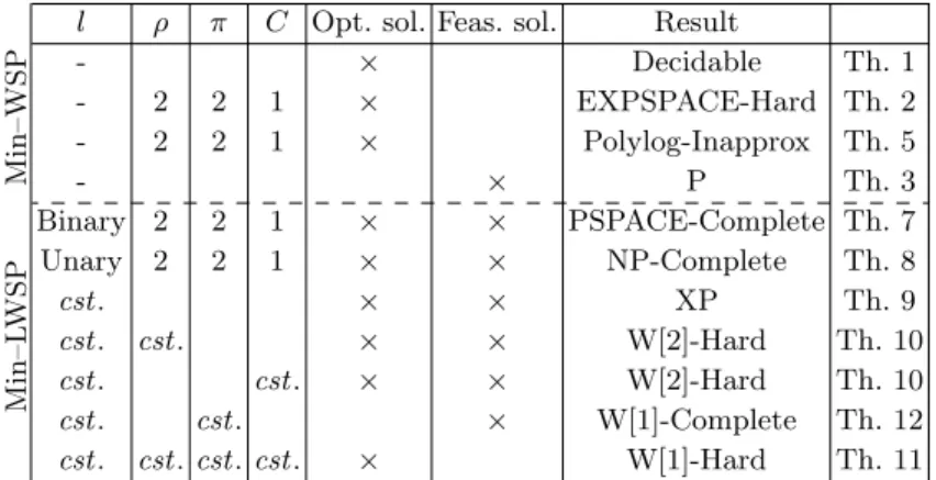
Table 1 summarizes the complexity results for Min–WSP and Min–LWSP given in Sections 3 and 4.
Table 1. Summary of the results of the paper. The four first lines concern Min–WSP and the others concern Min–LWSP. The four first columns indicate how the parameters of the problems are considerered for the complexity: a unary entry, a binary entry, a fixed constant or a fixed value. Note that l is not defined for Min–WSP thus for the four first lines. The columns Opt. sol. and Feas. sol. respectively specify if the results stands for the search of an optimal solution, the search of the existence of a feasible solution or both.
l ρ π C Opt. sol. Feas. sol. Result
Min–WSP - × Decidable Th. 1 - 2 2 1 × EXPSPACE-Hard Th. 2 - 2 2 1 × Polylog-Inapprox Th. 5 - × P Th. 3 Min–L WSP Binary 2 2 1 × × PSPACE-Complete Th. 7 Unary 2 2 1 × × NP-Complete Th. 8 cst . × × XP Th. 9 cst . cst . × × W[2]-Hard Th. 10 cst . cst . × × W[2]-Hard Th. 10 cst . cst . × W[1]-Complete Th. 12 cst . cst . cst . cst . × W[1]-Hard Th. 11
The hardness results for deciding the existence of a feasible solution of an instance of Min–LWSP immediately proves hardness of approximability for the optimization problem.
The next section is dedicated to the formal definitions of the terminology. In addition, it gives drawing conventions of this paper and details the parameters we focus on in the parameterized complexity study. Sections 3 and 4 are respectively dedicated to the studies of Min–WSP and Min–LWSP.
2
Definitions
This section is dedicated to the formal definitions of the terminology we use and of the problems we study in this paper.
2.1 The Petri Net Coverability problem
A Petri net is a triplet (P, T , M0) where P is the finite set of places and T is
the finite set of transitions. Each place may contain zero, one or more tokens. A state M maps P to N, each place x is associated with a non-negative number
M (x) of tokens. We write, using classical vector notation [18], M = P
x∈P
ax· x
where ax= M (x). We may possibly remove a place x from the sum if axis null.
Particularly, an empty state is denoted by ∅. M0is called the initial state of the
Petri net: it defines the initial number of tokens in each place. Each transition t ∈ T is a couple of states t− = P
x∈P
t−(x) · x and t+= P
x∈P
t−(x) · x, respectively
called the input state and the output state of t. The set of places for which t−(x) > 0 and the set of places for which t+(x) > 0 are respectively called the
input states and the output states. We denote the transition by t = t− → t+.
We say a state M0 covers another state M if and only if, for all x ∈ P, M0(x) ≥ M (x). Considering a state M of the Petri net, one can fire a transition t ∈ T if M covers the input state t−. We say t is enabled at M . In that case, the resulting state is M0 = P
x∈P
(M (x) − t−(x) + t+(x)) · x. We denote this by M ⇒t M0. In other word, firing a transition means transforming some tokens in the input places into tokens in the output places. Similarly, we can define a sequence T = (t1, t2, . . . , t|T |). This sequence is enabled at M if we can successively fire
all the transitions of T from t1 to t|T |. In that case, and if firing this sequence
produce the state M0, we write M ⇒T M0. Note that the sequence T may contain a transition t more than once.
We can now formally define the classical coverability problem in Petri nets. Problem 1 (Coverability). Given a Petri net (P, T , M0) and a target state C, is
there an enabled sequence T at M0 such that M0⇒T M and M covers C?
We represent an instance of this problem by a bipartite directed graph in which the places are circle nodes and the transitions are squared nodes. For each transition nodes t, we represent the input and output state using incoming and respectively outgoing arcs. An arc (x, t) (resp. (t, x)) is associated with the value t−(x) (resp. t+(x)). We omit this value when it is 1 and we omit the arc when
it is 0. For each target place, i.e. a place x for which C(x) 6= 0, is drawn with a double circle. A dashed outgoing arc, from x, is associated with the number C(x). Given a state M , M (x) is represented by a value inside the circle node x. An example is given on Figure 1.
2.2 The Weighted Petri Net Synthesis problem
The Minimum Weighted Synthesis Problem (Min–WSP) insert an optimization part to the previous problem. Each transition t ∈ T is associated with a non-negative weight ω(t) ∈ R+. In addition, the initial state M0 is always ∅, there
is not any token in any place. However, note that the Petri net may contain transitions for which the input state is empty.
We define the weight ω(T ) of a sequence T of transitions of T as the sum ω(T ) = P
t∈T
ω(t).
Problem 2 (Minimum Weighted Synthesis, Min–WSP). Given a Petri net (P, T , ∅), a weight function ω : T → R+ over the transitions and a target state C, return
3 x 2 y 2 z c t1 t2 2 2 3 2 6
Fig. 1. This figure illustrates an instance of the coverability problem: a Petri Net with four places x, y, z, c and two transitions t1= 2x + y → 2z + 3c and t2= z → 2c. The
initial state M0 is 3x + 2y + 2z. After firing t1, t2, t2 we obtain the state M = x + 7c
which is covering the target state 6c.
a enabled sequence T at ∅ of T such that ∅ ⇒T M , M covers C, and ω(T ) is
minimum.
In addition, we denote by FS–MWSP the problem of determining if there exists a feasible solution for an instance of Min–WSP.
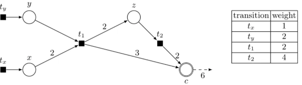
We use a representation similar to the classical Petri nets. We add a table indicating the weight of each transition. An example of a Min–WSP instance if is given in figure 2. x y z c tx ty t1 t2 2 2 3 2 6 transition weight tx 1 ty 2 t1 2 t2 4
Fig. 2. This figure illustrates a instance of Min–WSP. It is a Petri Net with four places x, y, z, c and four transitions tx= ∅ → x, ty= ∅ → y, t1= 2x + y → 2z + 3c and
t2= z → 2c. The initial state M0 is ∅. After firing (ty, ty, tx, tx, tx, tx, t1, t1) of weight
12 we obtain the state M = 7c which is covering the target state 6c.
2.3 Parametrized version of Min–WSP
In order to analyze the parametrized complexity of the Petri Net Synthesis prob-lem, we introduce four different parameters: ρ and π, respectively the maximum number of input and output tokens among all the transitions of T , C the size of the target state and l the number of transitions fired in a feasible solution. As
the three first are constraints on the instances, the last is a constraint on feasible solutions so we will threat it independently.
The two first parameters, ρ and π, limit the maximum number of input and output tokens. More formally,
ρ = max t∈T X x∈P t−(x) π = max t∈T X x∈P t+(x)
The third parameter on which we focus is the size C = P
x∈P
C(x) of the target state C. From a chemical perspective, these parameters model the limited number of reactants, products of reactions and the number of molecules we want to synthesize, which is likely to be small.
Finally, we define a fourth parameter l to limit the number of molecules we can buy and the number of reactions we can perform to synthesize the target molecules. As introducing this parameter changes the set of feasible solutions for an instance (see Example 1), we define an independent problem: Minimum Limited sequence Weighted Synthesis problem (Min–LWSP).
Example 1. We constraint the instance of Figure 1 by introducing a parameter l = 6 to limit the number of fired transitions. As a consequence the sequence T = (ty, ty, tx, tx, tx, tx, t1, t1) is not a feasible solution anymore as it contains
8 transitions. This constraint instance contains only one feasible solution: the sequence T0= (ty, tx, tx, t1, t2, t2) of weight 14.
Problem 3. Limited sequence Weighted Petri Net Synthesis problem (Min–LWSP). Given a Petri net (P, T , ∅), a weight function ω : T → R+ over the transitions, a target state C and an integer l, return a enabled sequence T at ∅ of T such that ∅ ⇒T M , M covers C, |T | ≤ l and ω(T ) is minimum.
Similarly to FS–MWSP, we define FS–MLWSP the problem of determining if there exists a feasible solution for an instance of Min–LWSP.
3
Min–WSP
In this section, we study the complexity, the approximability and the parame-terized approximability of Min–WSP.
3.1 Complexity and parameterized complexity
The two next theorems give an upper bound and a lower bound of the complexity of Min–WSP: the problem is decidable but EXPSPACE-hard.
Theorem 2. Min–WSP is EXPSPACE-hard even if π = ρ = 2 and C = 1.
Remark 1. The theorem 2 shows that Min–WSP is not easier if we fix the three parameters π, ρ and C. As a consequence, there is no parameterized results considering those three parameters.
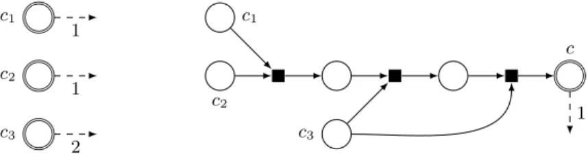
Proof. The proof of EXPSPACE-hardness is a reduction from the Petri net Cov-erability problem. This problem is EXPSPACE-hard [18,20]. Note that this result remains true if the Petri net satisfies π = ρ = 2 and if the target state contains a polynomial number C of tokens. We can create a equivalent instance with only one target token and π = ρ = 2 by firstly adding a new place c and a new transi-tion using all the C target tokens to create one token in c. Finally, transform this transition into C − 1 transitions and add C − 2 new places as shown in Figure 3 so that ρ remains 2. As C is polynomial, this transformation is polynomial too.
c3 c2 c1 2 1 1 c3 c2 c1 c 1
Fig. 3. Example of transformation from an instance (on the left) in which the target state C = c1+ c2+ 2 · c3 (and then C = 4) to an instance (on the right) satisfying
C = 1. The weight of every transition is 0.
Let I = ((P, T , M0), C) be an instance of the Petri net Coverability problem.
We create an instance J of Min–WSP in which the Petri net is (P, T ∪ {t}, ∅) in which we add a transition t which creates M0(x) tokens in x for every x ∈ P
from nothing. The weight of t is 1 and the weight of each other transition is 0. Finally, the target state is C. Then C is coverable in I if and only if there is a feasible solution of weight 1 in J . As a consequence the decision version of Min–WSP is EXSPACE-hard.
This last theorem shows that the problem of determining if there exists a feasible solution for an instance of Min–WSP is polynomial.
Theorem 3. FS–MWSP is polynomial.
Proof. In order to find a feasible solution, for each transition t for which the input state is empty, we mark all the output places of t. Then, for each transition t for which all the input places are marked, we mark all the output places. We repeat this marking operation either until no new place is marked. There is a feasible solution if and only if all the target places are marked.
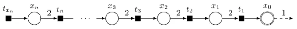
This means that it is conceivable to build approximation algorithms for this problem. However, we show in the next subsection a high inapproximability ratio. Moreover, note that Theorem 3 does not explain how to build a feasible solution. In fact, even if we can easily adapt the algorithm given in the proof to return such a solution, for some instances, no feasible solution contains a polynomial number of transitions. See, for example, the instance on Figure 4.
xn x3 x2 x1 x0
txn 2 tn 2 t3 2 t2 2 t1 1
. . .
Fig. 4. Example of instance for which the number of transitions is exponential. Indeed, in order to put a token in the place x0, we need to buy 2n tokens for xn using the
transition txn, then fire 2
n−1times the transition t
n, then fire 2n−2times the transition
tn−1, and so on until we fire once the transition t1. This sequence contains then 2n
transitions.
3.2 Approximability
We show in this subsection that Min–WSP cannot be approximated within a polylogarithmic ratio in polynomial time. Basically, the best ratio an approxi-mation algorithm may achieve is at least polynomial in the size of the instance. In order to prove this inapproximability result for Min–WSP, we build, in this subsection, a reduction from the MMSAhproblem.
Problem 4. Minimum Monotone Satisfying Assignment (MMSAh). Given
a set Y of boolean variables and a monotone boolean formula ϕ of depth h (this formula has h levels of altenating AND and OR gates, where the top levels is an AND gate), minimize the number of true variables such that ϕ is satisfied.
We respectively call D(ϕ) and C(ϕ) the set of OR and AND gates in the formula.
Theorem 4 ([26]). Unless P = NP, there is no polynomial approximation for MMSA3 with a ratio Q(log(|Y |), log(|D(ϕ)|), log(|C(ϕ)|)) where Q is any
poly-nomial.
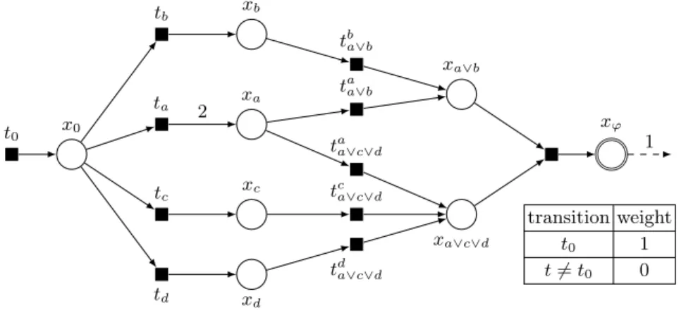
We now detail and prove a reduction from MMSAhto Min–WSP. An example
is given on Figure 5. Let I = (Y, ϕ) be an instance of MMSAh, we build the
following instance J :
– add one place x0and a transition t0= ∅ → x0;
– for each variable y, add one place xy and a transition ty = x0→ ly· xy where
ly is the number of literals y in ϕ;
– for each OR gate g =W
iϕi, where ϕi are either gates or variables, add, for
each i, a transition ti
g= xϕi→ xg;
– for each AND gate g =V
iϕi, where ϕi are either gates or variables, add a
transition tg=Pixϕi→ xg;
– set the target state to C = xg where g is the top level AND gate;
– set the weight of t0 to 1 and the weight of every other transition to 0.
x0 xa xb xc xd xa∨b xa∨c∨d xϕ t0 ta a∨b tba∨b taa∨c∨d tca∨c∨d td a∨c∨d ta tb tc td 2 1 transition weight t0 1 t 6= t0 0
Fig. 5. Example of reduction from MMSA2 to Min–WSP with the boolean formula
ϕ = (a ∨ b) ∧ (a ∨ c ∨ d).
Lemma 1. If there is a feasible solution for I with ω ≥ 1 true variables, there is a feasible solution for J of weight ω.
Proof. The solution consists in firing ω times t0 (this way, we put ω tokens in
the place x0) and then using all the transitions of the true gates and variables
in the formula, starting with the variables and the lower gates and terminating with the top level AND gate. The proof that, when a transition is fired, all the input places contain a token (and then that the solution is feasible) can be done by induction on the height of each gate.
Lemma 2. If there is a feasible solution for J of weight ω ≥ 1, there is a feasible solution for I with at most ω true variables.
Proof. Let T = (t1, t2, . . . , t|T |) be a feasible solution for J of cost ω ≥ 1. We
now prove that assigning true to all the variables y ∈ Y such that ty ∈ T is a
feasible solution for I of cost at most ω. Let f be the boolean function associating to each variable and each gate the value true or f alse. We have to check that f (g) is true where g is the top level AND gate.
Firstly, there are at most ω distinct variables for which the transition is fired in T . Indeed, in order to fire the transition tyassociated with the variable y ∈ Y ,
we have to fire the transition t0 of weight 1 first in order to put a token in x0.
As the weight of T is ω, there are at most ω variables set to true.
Secondly, for each 1 ≤ i ≤ |T | such that ti6= t0, the transition tiis associated
either with a variable y or a gate g. Considering how we set the true and false variables in I, if the transition is associated with a variable y, then f (y) is true. We now prove by induction on i that, on the other case, f (g) is true. Let ϕ(t) be the variable or the gate associated with the transition t, for t 6= t0. Similarly,
ϕ(x) is the variable or the gate associated to the place x, if x 6= x0. Note that
the first transition ti for which ti6= t0is necessarily associated with a variable.
We now assume that, for every j ≤ i, either tj= t0or f (ϕ(tj)) is true. We also
assume, without loss of generality that ti+1 6= t0 and that g = ϕ(ti+1) is an
OR gate: g = ϕ1∨ ϕ2∨ · · · ∨ ϕk. Thus, ti+1 has one input place x 6= x0 such
that ϕ(x) = ϕκ for some κ ∈ J1; kK (and ti+1 = t
ϕκ
g ). Before this transition is
fired, x contains a token otherwise T would not be a feasible solution for J . As x 6= x0, the token in x was added by a reaction tj 6= t0 for some j ≤ i and
ϕ(x) = ϕ(tj) = ϕκ. By the inductive hypothesis, f (ϕ(tj)) is true, then f (g) is
true. A similar argument occurs if g is an AND gate. Consequently, there is a feasible solution for I of cost at most ω.
Theorem 5. Unless P = NP, there is no polynomial approximation for Min– WSP with a ratio Q(log(|P|), log(|T |)) even if π = ρ = 2 and C = 1 where Q is any polynomial.
Proof. Let Q be a polynomial. We assume that the cost of an optimal solution for I is ω∗. We can use the previous reduction to build an instance J . By Lemmas 1
and 2, the cost of an optimal solution for J is ω∗. If there is a Q(log(n), log(m))-approximation for Min–WSP, we can use it to build a solution for J of cost at most Q(log(n), log(m)) · ω∗, and then use Lemma 2 to build a feasible solution for I of cost at most Q(log(n), log(m)) · ω∗.
Finally note that, in the reduction m = |C(φ)| + |D(φ)|(|D(φ)| + |C(φ)| + |Y |)+|Y | et n = 1+|C(φ)|+|D(φ)|+|Y |, thus there is a polynomial Q0such that
Q(log(n), log(m)) ≤ Q0(log(|Y |), log(|D(ϕ)|), log(|C(ϕ)|)). As a consequence, we have built a Q0(log(|Y |), log(|D(ϕ)|), log(|C(ϕ)|))-approximation for MMSAh.
By Theorem 4, this is a contradiction.
4
Min–LWSP
In this section, we study the complexity, the approximability and the parame-terized approximability of Min–LWSP.
4.1 Complexity
Theorem 6. The decision versions of Min–LWSP and FS–MLWSP are in PSPACE. Proof. Let K be any integer. We search for the existence of a feasible solution of weight less than K. To achieve this, we provide a non-deterministic algorithm that runs in polynomial space.
We start with a state where all the places are empty. At each iteration, we non-deterministically choose a transition t. If t is not enabled at the current state or if the maximum weight K is lower than the current weight, then return NO, otherwise, fire the t. If l + 1 transitions were fired, return NO. If the target state is covered, return YES. If none of those cases occur, we start a new iteration.
At each iteration, the algorithm must store, for each place, the number of tokens in that place. Those numbers are no more than l · π as a transition can produce at most π tokens. It must also store the current total weight and the number of the current transition, which are respectively no more than K and l. Consequently, this algorithm runs in polynomial space and Min–LWSP is in NPSPACE.
As PSPACE = NPSPACE [25], Min–LWSP is in PSPACE. The proof for FS–MLWSP is exactly the same except that we do not have to consider the weight.
Theorem 7. The decision versions of Min–LWSP and FS–MLWSP are PSPACE-complete, even if ρ = π = 2 and C = 1.
Proof. The proof of Theorem 1 of [18], page 287, gives a reduction from the Turing halting problem in polynomial space to the Reachability problem (and the Coverability problem) for 1-Conservative Petri nets with ρ = π = 2 and C = 1. The same reduction can be used to prove our theorem. Some states encode the tape and others encode the states of the automata. Each transition function is encoded by a transition of the Petri net of weight 0. As the machine cannot use more that P (|x|) cells of the tape, where P is a polynomial and x is the input word, it cannot use more than 2P (|x|)|Q| transitions where |Q| is the
size of the automata otherwise the machine loops indefinitely. Thus the Petri net must cover the target state by firing at most that number of transitions. The initial state of the Petri net of the proof of [18] encodes the word x written on the tape and the initial state of the automata. In this version, we add a transition t0
of weight 1 that creates that initial state from nothing. We can then transform t0 into multiple transitions as we did in Theorem 2 so that π remains 2. The
machine halts without using more than P (|x|) cells if and only if the Petri net covers the target state with at most 1 + 2P (|x|)|Q| transitions of total weight at
most 1.
Thus the decision version of Min–LWSP is PSPACE-hard. By Theorem 6, the decision version of Min–LWSP is PSPACE-Complete, even if ρ = π = 2 and C = 1.
In order to prove that FS–MLWSP is also PSPACE-hard, we must prevent the transition t0from being fired twice in a feasible solution. To do so, we add a
place x0as input of t0and a construction as the one given in Figure 4 so that we
need to fire at least 2P (|x|)+1|Q| transitions in order to put a token in the place
x0. We then set l = 2P (|x|)+1|Q| + 2P (|x|)|Q| + 1 so that any feasible solution
cannot place more than one token in x0and then cannot fire t0twice.
Theorem 8. If the encoding of l is unary, the decision versions of Min–LWSP and FS–MLWSP are NP-Complete, even if ρ = π = 2 and C = 1.
4.2 Parameterized complexity and approximability
We present in this section four theorems describing the parameterized complexity of Min–LWSP and FS–MLWSP. There are proved using reduction from and to the set cover problem and the partitioned clique problem.
Problem 5. Set Cover. Given an integer K, a set E and a set S ⊂ 2E, find a subset S0 of S covering E such that |S0| ≤ K.
Problem 6. Partitioned clique Given an undirected graph G = (V, E) and a partition V1, V2, . . . , Vk of V , find a clique of size k with exactly one node in each
set Vi.
Set Cover problem is W[2]-Complete with respect to the parameter K [8]. Partitioned clique problem is W[1]-complete with respect to the parameter k [23]. Theorem 9. Min–LWSP is XP with respect to the parameter l.
Proof. Indeed, one can search for an optimal solution by exhaustively enumerate all the mlsequences of transitions.
Theorem 10. FS–MLWSP is W[2]-hard with respect to the parameters l and ρ and is W[2]-hard with respect to the parameters l and C.
Proof of Theorem 10. This proof is an FPT reduction from the set cover problem parameterized with K. Let I = (K, E, S) be an instance of Set Cover. We now build an instance J of FS–MLWSP parameterized with l and ρ.
We create for each element e in E a place xe. For each set s in S, we create a
transition ts= ∅ → P e∈s
xe. The target state is C = P e∈E
xe. We finally set l = K.
This reduction satisfies ρ = 0. A feasible solution S0for I can be transformed into a feasible solution for J by firing every transition tsfor s ∈ S0 and, conversely,
from a feasible solution for J , we can build a feasible solution for I by selecting the sets for which the transition is fired. As this reduction is FPT with respect to K, FS–MLWSP is W[2] with respect to l and ρ.
If we now add to this instance a new place c and a new transition P
e∈E
xe→ c;
and if the target state is C = c, we get an instance of FS–MLWSP in which C = 1. Note that ρ does not polynomially depend on the parameter K. As this reduction is also FPT with respect to K, FS–MLWSP is W[2] with respect to l and C. Theorem 11. FS–MLWSP is W[1]-hard with respect to the parameters l, ρ, π and C.
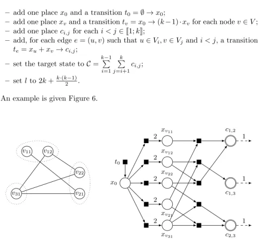
Proof. Given an instance I = (G, V1, V2, . . . , Vk) of Partitioned Clique, we now
– add one place x0and a transition t0= ∅ → x0;
– add one place xv and a transition tv= x0→ (k − 1) · xvfor each node v ∈ V ;
– add one place ci,j for each i < j ∈J1; kK;
– add, for each edge e = (u, v) such that u ∈ Vi, v ∈ Vj and i < j, a transition
te= xu+ xv → ci,j;
– set the target state to C =
k−1 P i=1 k P j=i+1 ci,j; – set l to 2k + k·(k−1)2 . An example is given Figure 6.
v11 v12 v22 v21 v31 t0 x0 xv11 xv12 xv22 xv21 xv31 c1,2 c1,3 c2,3 1 1 1 2 2 2 2 2
Fig. 6. Example of reduction from Partitioned Clique to FS–MLWSP. On the left, the three dashed ellipses describe the partition of the nodes.
This reduction is polynomial and l, C, ρ and π depends only on k. Thus it is FPT with respect to k.
If there is a clique (v1, v2, . . . , vk) of size k in G satisfying vi∈ Vifor i ∈J1; kK, there is a feasible solution for J consisting in buying k tokens for the place x0
with the transition t0, firing the k transitions tvi for i ∈ J1; kK and then firing the k·(k−1)2 transitions t(vi,vj) for i < j ∈J1; kK. Those transitions exist and are enabled as (v1, v2, . . . , vk) is a clique.
We now assume there is a feasible solution T = (t1, t2, . . . , t|T |) for J . It
satisfies |T | ≤ l. Let TV and TE be respectively the set of transitions {tv, v ∈ V }
and {te, e ∈ E}. Let (M0 = ∅, M1, M2, . . . , M|T |) be the successive states of J
after firing the transitions of T . Note that ∅ ⇒T M|T |, and, as a consequence, this
state M|T |contains at least C(ci,j) = 1 token in each place ci,j for i < j ∈J1; kK. Only the transitions of TE can create such tokens. As none of those transitions
TE. As l = 2 · k + k·(k−1)
2 , there are at most 2k transitions of {t0} ∪ TV in T . As
there must be a token in x0 before a transition of TV can be fired, there are at
most k transitions of TV in T .
In addition, there is, for each i ∈J1; kK, at least one node vi in Vi and an
integer l such that Ml(xvi) ≥ 1. Indeed, otherwise, no transition of TEplacing a
token in cjior cij for all j 6= i could have been fired. Thus, there are in T exactly
k transitions of TV. Each one is associated with one node vi∈ Vi for i ∈J1; kK. Finally, (v1, v2, . . . , vk) is a clique, otherwise, some transition t(vi,vj) would
not exist and consequently no token could have been placed in ci,j.
This conclude the reduction. FS–MLWSP is W[1]-Hard with respect to the parameters l, C, π and ρ.
We finally prove that FS–MLWSP belongs to the W[1] class if parameterized with l and π. We first give an intermediate lemma proving that, if l and π are fixed, we can consider that ρ and C are fixed too.
Lemma 3. There exists an FPT-reduction from FS–MLWSP parameterized with l and π to FS–MLWSP parameterized with l, π, ρ and C.
Proof. As there are at most l transitions in a feasible solution and as every transition may produce at most π tokens, a feasible solution may produce at most l · π tokens. Consequently, if C > l · π there is no feasible solution and the problem is solved. In addition, if a transition needs more than l · π input tokens, this transition may be removed from the instance as it is not possible to fire it. We then necessarily get an instance where C ≤ l · π and ρ ≤ l · π.
Theorem 12. FS–MLWSP is W[1]-complete with respect to the parameters l and π.
Due to its length, the complete proof is given in Appendix A. It is based on a reduction to the partitioned clique problem.
Remark 2. Note that Theorem 12 does not prove any parameterized result on Min–LWSP. Determining if Min–LWSP is W[1]-Complete with respect to l and π and with respect to l, ρ, π and C are open questions.
Finally, the complexity of the determing if there exists feasible solutions for Min–LWSP allows us conclude this section with the following corollary.
Corollary 1. Let Q by a polynomial.
– Unless P = PSPACE, there is no polynomial approximation for Min–LWSP with a ratio 2Q(|P|,|T |) even if ρ = π = 2 and C = 1.
– Unless P = NP, there is no polynomial approximation for Min–LWSP with a ratio 2Q(|P|,|T |) even if ρ = π = 2 and C = 1 and if the encoding of l is
unary.
– Unless FPT = W[1], there is no FPT approximation for Min–LWSP with ratio 2Q(|P|,|T |), with respect to l, ρ, π and C.
5
Conclusion
In this paper we present the Minimum Weight Synthesis problem, a variant of the classical Coverability problem introducing weights on transitions. We pro-vide a deep analysis of the complexity and parametrized complexity. Our results are summarized in table 1. They illustrate how hard this problem is even when most parameters are constrained. In the last section, we prove that using ap-proximation algorithm for solving this problem is not adequate as there is no constant ratio or small variable ratio approximation algorithm.
From a theoretical perspective, there are a few cases of parameterized com-plexity which are still open questions. In particular, theorems 10 and 11 provide W[1]-hard and W[2]-hard results. It would be interesting to find others reduc-tions to achieve completeness results.
From a more practical perspective, as the problem is hard to solve and to approximate, we should now study the different heuristic algorithms.
References
1. Reaxys. https://www.elsevier.com/solutions/reaxys, 2016. Elsevier.
2. Abdulla, P. A., and Mayr, R. Minimal cost reachability/coverability in priced timed petri nets. Lecture Notes in Computer Science (including subseries Lecture Notes in Artificial Intelligence and Lecture Notes in Bioinformatics) 5504 LNCS (2009), 348–363.
3. Abdulla, P. A., and Mayr, R. Computing optimal coverability costs in priced timed petri nets. Proceedings - Symposium on Logic in Computer Science (2011), 399–408.
4. Abdulla, P. A., and Mayr, R. Priced timed petri nets. Logical Methods in Computer Science 9, 4 (2013), 1–51.
5. Andersen, J. L., Flamm, C., Merkle, D., and Stadler, P. F. Maximizing output and recognizing autocatalysis in chemical reaction networks is NP-complete. Journal of Systems Chemistry 3, 1 (2012), 1–9.
6. Angeli, D., De Leenheer, P., and Sontag, E. A Petri Net approach to the study of persistence in chemical reaction networks. Mathematical Biosciences 210, 2 (2007), 598–618.
7. Bøgevig, A., Federsel, H.-J., Huerta, F., Hutchings, M. G., Kraut, H., Langer, T., L¨ow, P., Oppawsky, C., Rein, T., and Saller, H. Route design in the 21st century: The ic synth software tool as an idea generator for synthesis prediction. Organic Process Research & Development 19, 2 (2015), 357–368. 8. Downey, R., and Fellows, M. Parameterized complexity, vol. 3.
Springer-Verlag, 1999.
9. Eigner-Pitto, V., Huerta, F. F., Hutchings, M. G., Saller, H., and Loew, P. Reaction prediction tools for both idea generation in new synthesis route plan-ning and for de novo molecule design. In 12th German Conference on Chemoin-formatics (2016).
10. Finkel, A. The minimal coverability graph for Petri nets. In Advances in Petri Nets 1993. Springer Berlin Heidelberg, 1993, pp. 210–243.
11. Finkel, A., and Leroux, J. Recent and simple algorithms for Petri nets. Software and Systems Modeling 14, 2 (2015), 719–725.
12. Genrich, H., K¨uffner, R., and Voss, K. Executable Petri net models for the analysis of metabolic pathways. International Journal on Software Tools for Technology Transfer 3, 4 (2001), 394–404.
13. Hastings, J., de Matos, P., Dekker, A., Ennis, M., Harsha, B., Kale, N., Muthukrishnan, V., Owen, G., Turner, S., Williams, M., and Steinbeck, C. The chebi reference database and ontology for biologically relevant chemistry: enhancements for 2013. Nucleic Acids Research 41, D1 (2012), D456.
14. Heiner, M. Preface: Petri nets for systems and synthetic biology. Natural Com-puting 10, 3 (2011), 987–992.
15. Hofest¨adt, R. A petri net application to model metabolic processes. Systems Analysis Modelling Simulation 16, 2 (1994), 113–122.
16. Horvath, D., and Jeandenans, C. Molecular similarity and virtual screening. in silico methods to retrieve active analogs in the context of discovering therapeutic compounds. Actualit´e Chimique 9 (2000), 64–67.
17. Johnson, A. P., and Marshall, C. Starting material oriented retrosynthetic analysis in the lhasa program. 2. mapping the sm and target structures. Journal of chemical information and computer sciences 32, 5 (1992), 418–425.
18. Jones, N. D., Landweber, L. H., and Edmund Lien, Y. Complexity of some problems in Petri nets. Theoretical Computer Science 4, 3 (1977), 277–299. 19. Koch, I. Petri nets–a mathematical formalism to analyze chemical reaction
net-works. Molecular Informatics 29, 12 (2010), 838–843.
20. Lipton, R. J. The Reachability Problem Requires Exponential Space. Tech. rep., Yale Research Report #63, 1976.
21. Nouleho, S., Barth, D., David, O., Watel, D., and Weisser, M. A new definition of molecule similarity to determine molecular construction. In Poster in 12th German Conference on Chemoinformatics (2016).
22. Petri, C. A. Kommunikation mit Automaten. PhD thesis, Universit¨at Hamburg, 1962.
23. Pietrzak, K. On the parameterized complexity of the fixed alphabet shortest common supersequence and longest common subsequence problems. Journal of Computer and System Sciences 67, 4 (2003), 757–771.
24. Reddy, V. N., Mavrovouniotis, M. L., and Liebman, M. N. Petri net rep-resentations in metabolic pathways. Proceedings / ... International Conference on Intelligent Systems for Molecular Biology ; ISMB. International Conference on Intelligent Systems for Molecular Biology 1 (1993), 328–36.
25. Savitch, W. J. Relationships between nondeterministic and deterministic tape complexities. Journal of Computer and System Sciences 4 (1970), 177–192. 26. Watel, D., and Weisser, M.-A. A note on the inapproximability of the Minimum
Monotone Satisfying Assignment problem. Tech. rep., HAL, https://hal.archives-ouvertes.fr/hal-01377704, 2016.
A
Proof of Theorem 12
Theorem 12. FS–MLWSP is W[1]-complete with respect to the parameters l and π.
Proof. By Lemma 3 and Theorem 11, we have to prove that FS–MLWSP is W[1] with respect to l, ρ, π and C. To do so, we describe a reduction to the partitioned clique problem. Let I = ((P, T , ∅), ω, C, l) be an instance of FS–MLWSP. We assume that I contains a fake transition t0 such that t−0 = t
+
0 = ∅ so that I
contains a feasible solution of size lower than l if and only if it contains a feasible solution of size exactly l. We now create an instance J = (G, V1, V2, . . . , Vl, Vl+1)
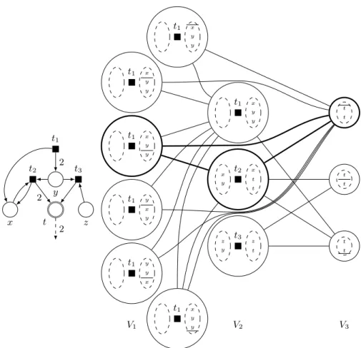
of the partitioned clique problem such that J contains a feasible solution if and only if I does. An example is given in Figure 7.
In the remaining of this proof, given a state M , the ordered set of states {α1, α2, . . . , αk} is called a decomposition of M if and only if P
k
j=1αj = M .
The state αj may be empty.
Let t be a transition of I. For each i ∈J2; lK, we create at most (i − 1)ρ·
(l − (i + 1))π nodes in V
i, one per decomposition of t− in i − 1 states and per
decomposition of t+ in l − i + 1 states. If t− = ∅, we also create at most lπ
nodes in V1, one per decomposition of t+ into l states. Finally, we add at most
lC nodes to V
l+1, one for each decomposition of C into l sets. For example, in
Figure 7, t−1 = ∅ and t+1 = x + 2y. We add six nodes to V1 as there are six
possible decompositions of t+i into 2 states : {∅, x + 2y}, {x, 2y}, {x + y, y} and the symmetrical decompositions. Note that the number of nodes in G is FPT with respect to the parameters l, ρ, π and C.
Let i < j ∈ J1; lK, and vi ∈ Vi and vj ∈ Vj be two nodes of G. The node
vi is associated with a transition ti, a decomposition of t−i and a decomposition
{αi+1, αi+2, . . . , αl+1} of t+i . Similarly, the node vjis associated with a transition
tj, a decomposition {β1, β2, . . . , βj−1} of t−j and a decomposition of t +
j. We add
to G the edge (vi, vj) if and only if αj covers βi.
Similarly, let i ∈J1; lK, and vi∈ Vi and vl+1 ∈ Vl+1 be two nodes of G. The
node vi (respectively vl+1) is associated with a transition ti, a decomposition
of t−i and a decomposition {αi+1, αi+2, . . . , αl+1} of t+i (resp. a decomposition
{β1, β2, . . . , βl} of C). We add to G the edge (vi, vl+1) if and only if αl+1covers βi.
For example, in Figure 7, the last node of V1 and the second node of V2
are respectively associated with the decomposition {x + 2y, ∅} of t+1 and the decomposition {x + y} of t−2. The two nodes are linked as x + 2y covers x + y.
We now prove that J contains a feasible solution if and only if I contains an enabled sequence at ∅ with exactly l transitions such that the resulting state covers C.
We first assume there is a clique of G containing a node viof Vifor every i ∈
J1; l+1K. Let T = (t1, t2, . . . , tl) be the sequence such that tiis the transition asso-ciated with vifor i ≤ l. Let {βi,1, βi,2, . . . , βi,i−1} and {αi,i+1, αi,i+2, . . . , αi,l+1}
be respectively the decompositions of t−i and t+i associated with vi and let
x y z t t1 t2 t3 2 2 2 V1 V2 V3 t1 x y y t1 x y y t1 x y y t1 y x y t1 y y x t1 x y y t1 x y y t2 x y x t t t3 z y z t t t t t t t
Fig. 7. Example of reduction from an instance I of FS–MLWSP with l = 2 on the left to an instance J of Partitioned Clique on the right. Due to lack of space, the fake transition is not part of I. Each node of the clique instance is either a transition t with decompositions of t−(on the left) and t+(on the right) or an decomposition of C into 2 states. The sequence (t1, t2) is a feasible solution of I. The bold clique on the right
is a feasible solution of J associated with that sequence.
We now show that T is enabled at ∅. As v1∈ V1, then t−1 = ∅ and t1is enabled at
∅. Let i ∈J1; l − 1K. As (v1, v2. . . vi, vi+1) is a clique of G, then, by construction, αj,i+1covers βj,i+1 for every j ∈J1; iK. For each place x of P :
i X j=1 (t+j(x) − t−j(x)) ≥ i X j=1 αj,i+1(x) + i X k=j+1 αj,k(x) + j−1 X k=1 βk,j(x) ≥ i X j=1 αj,i+1(x) + X j<k≤i (αj,k(x) − βj,k)(x) ≥ i X j=1 αj,i+1(x) = t−i+1(x)
Consequently, for every i ∈J1; lK, (t1, t2, . . . , ti) is enabled at ∅. Finally, we
can similarly show that
l P j=1 (t+j(x) − t−j(x)) ≥ l P j=1 αj,l+1(x) and, as (vi, vl+1) is an
edge of G for i ≤ l + 1, then, by construction,
l P j=1 αj,l+1(x) ≥ l P j=1 Cj(x) = C(x)
for every place x. Thus, when firing T , the resulting state covers C and T is a feasible solution of I.
We now assume there exists such a feasible solution T = (t1, t2, . . . , tl) of
I and prove J contains a clique of size l + 1. Let γi,j, for i < j ∈ J1; lK be the states describing the tokens produced by ti and consumed by tj ; let γi,l+1
be the tokens produced by ti, not consumed by any next transition and used
to cover C ; and finally let γi,l+10 be the not consumed tokens of t+i that are not used to cover C. Thus, we have firstly t+i =
l+1 P j=i+1 γi,j ! + γ0i,l+1, secondly t−j = j−1 P i=1
γi,j and thirdly l
P
i=1
γi,l+1 = C. For each set Vi with i ≤ l, we select
the node vi associated with ti, the decomposition {γj,i, j ≤ i − 1} of t−i and the
decomposition {γi,i+1, . . . , γi,l, γi,l+1+ γ0i,l+1} of t +
i . We finally choose the node
vl+1 of Vi+1 associated with the decomposition {γj,l+1, j ≤ l} of C. If i < j ≤ l,
then γi,j is the j-th state of the decomposition of t+i and the i-th state of the
decomposition of t−j. By construction the edge (vi, vj) belongs to G. Moreover, if
i ≤ l, the last state γi,l+1+ γi,l+10 of the decomposition of t +
i covers the i-th state
γi,l+1 of the decomposition of C. By construction the edge (vi, vl+1) belongs to
G. Consequently, {v1, v2, . . . , vl+1} is a clique of size of l + 1 in J .
As a result, FS–MLWSP is W[1] with respect to l and π. By Theorem 11, it is W[1]-Complete.