Coastal Ocean Forecasting: science foundation and user benefits

(1)

Full Terms & Conditions of access and use can be found at

http://www.tandfonline.com/action/journalInformation?journalCode=tjoo20

Download by: [University of Liege] Date: 08 January 2016, At: 01:34

Journal of Operational Oceanography

ISSN: 1755-876X (Print) 1755-8778 (Online) Journal homepage: http://www.tandfonline.com/loi/tjoo20

Coastal Ocean Forecasting: science foundation

and user benefits

V.H. Kourafalou, P. De Mey, J. Staneva, N. Ayoub, A. Barth, Y. Chao, M. Cirano,

J. Fiechter, M. Herzfeld, A. Kurapov, A.M. Moore, P. Oddo, J. Pullen, A. van der

Westhuysen & R.H. Weisberg

To cite this article: V.H. Kourafalou, P. De Mey, J. Staneva, N. Ayoub, A. Barth, Y. Chao,

M. Cirano, J. Fiechter, M. Herzfeld, A. Kurapov, A.M. Moore, P. Oddo, J. Pullen, A. van der Westhuysen & R.H. Weisberg (2015) Coastal Ocean Forecasting: science foundation and user benefits, Journal of Operational Oceanography, 8:sup1, s147-s167, DOI: 10.1080/1755876X.2015.1022348

To link to this article: http://dx.doi.org/10.1080/1755876X.2015.1022348

Francis. Published online: 09 Jun 2015.

Submit your article to this journal Article views: 273

View related articles View Crossmark data

(2)

Coastal Ocean Forecasting: science foundation and user bene

ﬁts

V.H. Kourafaloua,o*, P. De Meyb,o, J. Stanevac, N. Ayoubb, A. Barthd,o, Y. Chaoe,f,o, M. Ciranog,o, J. Fiechterh, M. Herzfeldi,o, A. Kurapovj,o, A.M. Mooreh, P. Oddok,o, J. Pullenl,o, A. van der Westhuysenm,oand R.H. Weisbergn

a

University of Miami, Rosenstiel School of Marine and Atmospheric Sciences, Miami, FL, USA;bLaboratoire d’Etudes en Géophysique et Océanographie Spatiales, Toulouse, France;cInstitute for Coastal Research, Helmholtz-Zentrum, Geesthacht, Germany;dGHER, MARE, AGO, University of Liège, Belgium;eRemote Sensing Solutions, Pasadena, California, USA;fUniversity of California, Joint Institute for Regional Earth System Science and Engineering, Los Angeles, CA, USA;gFederal University of Bahia, Tropical Oceanography Group, Institute of Physics, Brazil;hUniversity of California Santa Cruz, Department of Ocean Sciences, CA, USA;iCSIRO, Hobart, Australia;

j

Oregon State University, College of Earth, Oceanic, and Atmospheric Sciences, Corvallis, OR, USA;kIstituto Nazionale di Geoﬁsica e Vulcanologia, INGV, Bologna, Italy;lStevens Institute of Technology, Hoboken, NJ, USA;mNOAA/NCEP/EMC/Marine Modelling and Analysis Branch, College Park, MD, USA;nUniversity of South Florida, College of Marine Science, St. Petersburg, FL, USA;oCoastal and Shelf Seas Task Team Member, GODAE OceanView

The advancement of Coastal Ocean Forecasting Systems (COFS) requires the support of continuous scientiﬁc progress addressing: (a) the primary mechanisms driving coastal circulation; (b) methods to achieve fully integrated coastal systems (observations and models), that are dynamically embedded in larger scale systems; and (c) methods to adequately represent air-sea and biophysical interactions. Issues of downscaling, data assimilation, atmosphere-wave-ocean couplings and ecosystem dynamics in the coastal ocean are discussed. These science topics are fundamental for successful COFS, which are connected to evolving downstream applications, dictated by the socioeconomic needs of rapidly increasing coastal populations.

Introduction

The development and evolution of Coastal Ocean Forecast-ing Systems (COFS) are largely dependent on both techno-logical and scientific advances, as well as on user needs. Continuous monitoring, in tandem with numerical model-ling techniques, over a range of spatial and temporal scales are fundamental components for the success of COFS. Integrated coastal observing and modelling systems have been emerging, progressively combined with regional and global systems, substantially advancing the quality of coastal forecasts and the services they can provide in support of societal and economic needs. Such activities are supported by international coordination under the Coastal Ocean and Shelf Seas Task Team (COSS-TT) within GODAE OceanView http://godae-oceanview.org. Examples of integrated systems and supporting approaches are given in a companion paper (Kourafalou et al. 2015). Here, the focus is on specific science issues and applications that drive the scientific developments which in turn enable COFS.

An adequate COFS should be able to monitor, predict and disseminate information about the coastal ocean state and thus cover a wide range of coastal processes. These include: mesoscale and sub-mesoscale shelf break

exchanges, shelf dynamics, fronts, connectivity, slope cur-rents, storm surges, tides, internal waves, surface waves, swell, upwelling, transport of nutrients, sediments and pol-lutants, estuarine processes, river plumes, and topographic controls on circulation. The land-sea interaction is gov-erned by coastal runoff and the resulting buoyancy-driven circulation and material transport. Air-sea interaction gen-erally occurs at short time and small space scales, driven by local orographic features and/or temperature differences between land and sea, which modulate and modify the large scale atmosphericﬂow.

Several components are needed to achieve these goals: a multidisciplinary, multiscale observational network; a state of the art modelling suite integrating the primitive equations and solving explicitly for the particular physical processes characterizing the coastal area; a robust data assimilation scheme accounting for anisotropy and complex cross correlations between errors in environ-mental variables; and a suite of dissemination tools able to scientiﬁcally integrate the information collected and transform it into products serving the community (scien-tists, policy makers, maritime stakeholders).

Coastal ocean disciplines are still advancing along active research topics. This evolution requires the

*Corresponding author. Email:vkourafalou@rsmas.miami.edu

This is an Open Access article distributed under the terms of the Creative Commons Attribution License (http://creativecommons.org/Licenses/by/4.0/), which permits unrestricted use, distribution, and reproduction in any medium, provided the original work is properly cited.

Journal of Operational Oceanography, 2015

Vol. 8, No. S1, s147–s167, http://dx.doi.org/10.1080/1755876X.2015.1022348

(3)

development of adequate observational networks to monitor and further understand the coastal ocean. Advanced understanding should provide new processes to be implemented and/or parameterized in ocean models to cover the observational gaps, but also to study the whole coastal ocean system and interactions that are impossible to solve analytically. Numerical models have limitations due to intrinsic errors, thus data assimilation schemes must be developed in parallel, accounting for the new pro-cesses and scales required to correct and drive the numeri-cal results. Finally, methods integrating the very complex resulting information obtained in simple and usable ways must be developed.

The goal of this paper is to discuss areas where scienti-fic progress is crucial for the development of COFS and the expected benefits that COFS can provide to the society at large and to specific users. The next section focuses on four major scientific aspects that are currently active areas of research: downscaling, coastal data assimilation and two types of inter-disciplinary couplings (circulation-waves, physics-biogeochemistry). This is followed by a discussion on a broad range of applications that are closely linked to the key science areas, while targeting user needs, with a focus on societal benefits. Concluding remarks focus on advances and benefits.

Science in support of coastal forecasting Downscaling the ocean estimation problem

The coastal ocean circulation is driven by a combination of local (winds, atmosphericfluxes, land drainage and tides) and deep-ocean forcings (along the shelf slope). Both of these influences must be included in COFS. Downscaling is accepted as the preferred methodology to propagate the large scale dynamics into COFS, through boundary con-ditions from Global Ocean Forecasting Systems (GOFS) (Auclair et al. 2001;Dombrowsky et al. 2009). The bound-ary conditions must capture relevant far-field phenomena, such as swells from distant storms in wave models, or ther-modynamic gradients and tidal information in circulation models. The forcing data and the representation of the coastal model geometry must be also appropriately scaled, with details that are often missing from the outer model.

Needs in boundary conditions, topography and forcing functions

An important downscaling issue arises from the fact that the large-scale solution is unbalanced with respect to the local physics of the embedded model, due to the different resolutions, bathymetries, numerical boundary conditions, etc. Simple interpolation may lead to problems, such as triggering unrealistic gravity transients. An assessment of

the sensitivity of the prescribed values imposed is generally recommended since the parent models may have different conﬁgurations, regarding their physics or even the space and time resolution of the outputs used (Kourafalou et al. 2009; Marta-Almeida et al. 2013a, Guillou et al. 2013). The added value of nesting in GOFS, versus using climato-logical or open boundary conditions is noted (De Mey et al. 2009;Zamudio et al. 2011).

A multi-nested downscaling approach is often employed, which involves the construction of one or more models of increasing spatial resolution, each nested inside the other and receiving information repre-senting the larger scale dynamics from the coarser model via open boundary conditions (OBCs). This can be accomplished in a one-way sense where information is only propagated toward higher resolution, or a two-way interaction where the ﬁne scale (or ‘child’) model delivers information back to the larger scale (or‘parent’) model (Mason et al. 2010; Debreu et al. 2012). The OBCs are crucial in such a transfer of information. However, the OBC problem is ill-posed, and no perfect boundary condition exists (Oliger & Sundstrom 1978). Fortunately, a large amount of literature exists on the subject, so the issues are clearly articulated (Marsaleix et al. 2008;Herzfeld et al. 2011).

Since OBCs are not perfect, the information that they deliver to the model interior often contains error. If the boundary tries to impose information that is strongly in conflict with what the model is attempting to do in the interior, then over-specification error results which often leads to instability or spurious boundary re-circulations. If insufficient information is delivered at the boundary, then under-specification error results and interior solutions can diverge from observations. Typically, attempts to mini-mize errors are made by radiating signals approaching the boundary from the interior out of the domain (Blumberg & Kantha 1985; Flather 1988). The typical use of a no-gradient condition for baroclinic velocity gives a non-conservative or inconsistent boundary cell. The use of a correctly implemented Dirichlet condition can lead to an unconstrained sea level (i.e. no OBC required), which can respond perfectly to incoming and outgoing pertur-bations and is conservative (Herzfeld & Andrewartha, 2012).

Implementation of the OBC equation (i.e. relative pos-ition of the normal velocity boundary face relative to the boundary cell center) is important, as it has been shown that the same boundary equation yields different solutions when implemented differently (Herzfeld 2009). These OBCs are often supplemented with sponge zones where friction is increased, ﬂow relaxation schemes to combine external data and model solutions or nudging zones to relax solutions to external data, primarily to improve stab-ility (Treguier et al. 2001;Martinsen and Engedahl 1987; Marchesiello et al. 2001). Applications using two way

(4)

nesting are gaining popularity (Jouanno et al. 2008; Cail-leau et al. 2008;Debreu & Blayo 2008). These approaches still have issues regarding conservation, which can be achieved at the expense of variable continuity, or can be a source of instability, particularly for non-aligned bathy-metries and meshes (Cailleau et al. 2008; Debreu et al. 2012). However, the advantage of the approach is that indi-vidual nests are associated with their own time-step, which can improve computational efﬁciency.

Obtaining sufficiently detailed and representative bathy-metric data needed for COFS models is both critical and a challenge. Whereas in oceanic applications bathymetric sources such as ETOPO1 (1arc-min horizontal resolution, vertical accuracy within 10 m) may be sufficient, higher-res-olution data are required for the coast. In the U.S, the most reliable bathymetric data source is from the National Oceanic and Atmospheric Administration (NOAA) VDatum project, combining bathymetric (sounding) and topographic (LIDAR) data. Another challenge is that coastal topography and bathymetry change on both intra-and inter-storm scales (e.g. bar formation during severe winter storms). It is, therefore, challenging to establish representative bathymetry in coastal models. Although it is possible to include morphological processes such as erosion and breaching, it is operationally unfeasible at present. Modelling at coastal scales also increases demands on atmospheric forcings: higher spatial resolutions and accurate land models (e.g. North American Mesoscale system, NAM, from NOAA’s National Centers for Environ-mental Prediction, NCEP) are required to capture coastal features. Marine meteorological processes, such as land-sea breezes, and river inflows become important in the coastal oceanic models, and must be captured adequately.

Examples of downscaling to resolve reefs and estuaries The Greater Barrier Reef (GBR) in Australia is a unique system, associated with its own set of speciﬁc dynamics that require a downscaling approach. Scales from the open ocean to the reef (from kilometers to meters) are seamlessly addressed through the eREEFS system (Schiller et al. 2014; Kourafalou et al. 2015). Within the GBR, the low frequency sea level response is primarily generated by wind stress within the lagoon (Burrage et al. 1991; Brinkman et al. 2002). From a downscaling perspective, using open bound-aries, this implies the use of a passive open boundary. However, the tides are large and warrant the use of an active boundary. OBCs with no or single relaxation time-scales struggle to reconcile these requirements; hence, a dual relaxation method OBC is implemented to sequentially represent the dynamics at these two different time-scales (Herzfeld & Andrewartha 2012).

The Florida Keys in the US are characterized by unique interactions between a long reef system and a boundary current. A rich eddyﬁeld associated with the meandering

Gulf Stream has a direct influence on reef flows and the replenishment of coral reef fishes, which are resolved through a downscaling approach from the global to the regional (Gulf of Mexico) and the reef scale (Kourafalou and Kang 2012;Sponaugle et al. 2005).

Forecasting estuarine circulation is in high demand, especially in regions of high population density like the San Francisco Bay/Estuary, largest estuary on the US Pacific coast and the largest wetland habitat in the western US. This system is modeled by the Semi-implicit Eulerian-Lagrangian Finite-Element (SELFE) modelling system (Figure 1). SELFE is an unstructured-grid model designed for the effective simulation of 3D baroclinic circu-lation across river-to-ocean scales (Zhang & Baptista, 2008). Horizontal resolution at the coastal boundary is 1km, increasing to 10 m in the estuary. A regional mesos-cale atmospheric model (the US Navy’s Coupled Ocean-Atmosphere Mesoscale Prediction System, COAMPS) provides atmospheric forcing. Boundary con-ditions outside the Golden Gate bridge are derived from a California coastal model (3 km horizontal resolution and 40 vertical layers) based on the Regional Ocean Model-ling System ROMS, http://myroms.org, extensively vali-dated using field observations (Hodur et al. 2002; Doyle et al. 2009;Shchepetkin & McWilliams 2005;Chao et al. 2008;Chao et al. 2009;Ramp et al. 2009;Wang et al. 2009). The influence of the coastal ocean on the bay/estuary circulation and variability is clearly shown in Figure 1. The tides entering through the Golden Gate can raise the San Francisco Bay water level as high as 2 m (not shown). Figure 1 shows model to data agreement that tidal induced salinity variations can be as large as 3. In addition to tidal fluctuations, the Bay/Estuary system also exhibits significant variability on time scales from days to years, presumably forced by a combination of river discharge, atmospheric forcing and coastal ocean circulation.

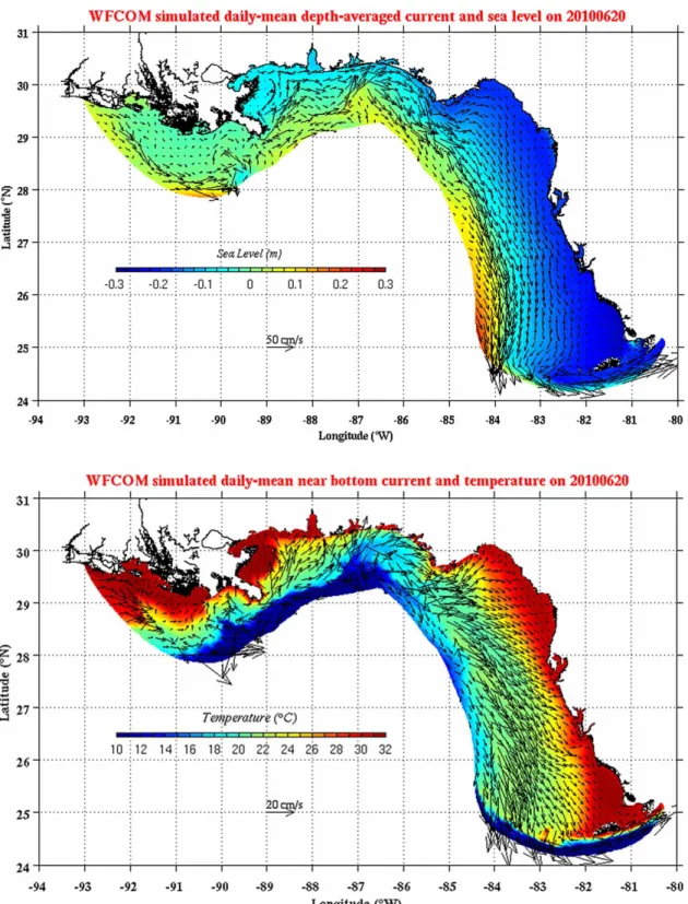
For the eastern Gulf of Mexico, the utility of down-scaling from the deep ocean, across the continental shelf and into the estuaries has been demonstrated (Zheng & Weisberg 2012). The unstructured, Finite Volume Coastal Ocean Model (FVCOM), e.g. Chen et al. (2003), wasﬁrst nested in the Global Hybrid Coor-dinate Ocean Model HYCOM, http://hycom.org, e.g. Chassignet et al. (2009), and eight tidal constituents were added along the open boundary. Along with hind-cast simulations that were quantitatively assessed against available in-situ observations, the model evolved to producing daily, automated nowcasts/fore-casts (WFCOM, West Florida Coastal Ocean Model, sub-sequently nested into the regional 1/25° Gulf of Mexico HYCOM, Figure 2). Horizontal resolution varies from that of HYCOM along the open boundary to 150 m in the estuaries. Local forcing includes surface winds and heat ﬂuxes from NOAA/NCEP NAM reanalyses Journal of Operational Oceanography s149

(5)

and river inﬂows. This model is an important step toward future downscaling to resolve inlets and shipping chan-nels, as for the adjacent Tampa Bay system (Zhu et al. 2014a,b). Such further downscaling may be useful when deep-ocean inﬂuences could drive contaminants from distant regions to an estuary or when species may migrate between different estuarine or shelf habitats. Under such scenarios the ability to resolve the principal

inlets that serve as mass conveyances and include sedi-ment dynamics may be important.

Coastal data assimilation and prediction

Data assimilation (DA) frameworks have been used in coastal ocean models to control the model trajectory and minimize errors, toward enhancing the model’s predictive Figure 1. (Top): Schematic diagram showing the one-way coupling between a structured grid ROMS off the California coast (left) and an unstructured grid SELFE over the San Francisco Bay/Estuary and lower Sacramento River (right). The left panel shows ROMS simulated SST. The middle panel shows the triangle unstructured grids on both sides of the Golden Gate bridge (narrowest passage on grid). The right panel shows the bottom topography (in meters) used by both ROMS and SELFE, with the thick black line representing the coupling bound-ary between ROMS and SELFE. (Bottom): Time series of water surface salinity as measured near Golden Gate (blue lines) and simulated by SELFE (red lines) during June-July 2009. Solid lines: hourly; dashed-circles: daily averages.

(6)

Figure 2. Snapshots on 20 June 2010 from a year-long WFCOM hindcast simulation. (Top): Daily and vertically averaged current vel-ocity superimposed on sea surface height. (Bottom): daily averaged near-bottom velvel-ocity and temperature. The coherent southward oriented circulation seen on the west Florida continental shelf is a consequence of a prolonged Gulf of Mexico Loop Current interaction with the shelf slope near the southwest corner of the model domain. The relative high sea level perturbation seen near the southwest corner (~25N, 84W) propagated to the north and west setting up a geostrophic current on the shelf itself, and left-hand turning in the bottom Ekman layer resulted in a pronounced upwelling that extended across the entire shelf, resulting in cold bottom water right up to the shoreline.

Journal of Operational Oceanography s151

(7)

capabilities. These topics are discussed below. Such frame-works have also been used for array design (including Observing System Experiments/Observing System Simu-lation Experiments; OSE/OSSEs) and probabilistic fore-casting (Kourafalou et al. 2015).

Accounting for model uncertainties

Many factors contribute to errors in coastal ocean model forecasts. These may include: imperfect atmospheric forcing fields; errors in boundary conditions propagating inside the finer scale model domain; bathymetric errors (more consequential in coastal regions); insufficient hori-zontal and vertical resolution and numerical noise and bias; errors in parameterizations of atmosphere-ocean inter-actions and sub-grid turbulence; intrinsic limited model pre-dictability (strong non-linearity), etc. To improve the quality of prediction, the model estimates are combined with avail-able data by means of DA. Many differentflavors of DA have been developed, tested, and implemented in numerical weather prediction and ocean forecasting. Some methods, including Optimal Interpolation (OI), 3-dimensional vari-ational (3DVAR), and Ensemble Kalman Filter (EnKF), provide instantaneous corrections to the present ocean esti-mate sequentially, at relatively short time intervals (several hours in the context of a shelf scale model) (Oke et al. 2002;Li et al. 2008a;Evensen 2003). The 4-dimensional variational (4DVAR) DA method finds corrections to model inputs (possibly including initial conditions, atmos-pheric forcing, boundary conditions, and errors in the dyna-mical equations) by minimizing the model-data misfit over a relatively large interval between the recent past and the present time (3–10 days in context of shelf and regional scale models) (Bennett 2002;Moore et al. 2011a;Kurapov et al. 2011). In addition to the nonlinear forecast model, 4DVAR utilizes the corresponding tangent linear and the adjoint codes (Talagrand & Courtier 1987; Moore, 1991; Errico & Vukićević 1992). The main advantage is that the observational error is filtered not only by interpolation in space, but also in time.

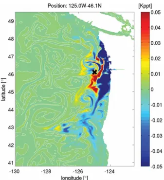
Since observations are often sparser in coastal regions that in the open ocean, in particular considering the short space/time scales of error processes, error covariances for the model estimates are critical since they provide interp-olation between the sparse observations, smoothing of the DA correction, and dynamical constraints on the correction ﬁelds (Kourafalou et al. 2015). In the coastal ocean, these covariances may be strongly inhomogeneous due to the coastal dynamics. For instance, large river plumes are associated with strong vertical and horizontal variability in stratiﬁcation and water properties. To account for this spatial and temporal variability, the model error covariance may be computed using an ensemble of simulations. An example is given inFigure 3, around the Columbia River (US West coast).

In order to guide the implementation of the DA scheme, background errors and model uncertainties must be charac-terized, both physically and statistically. This is demon-strated through an example from the Bay of Biscay (Northeast Atlantic), where an Ensemble-based DA method is being implemented to improve the realism of regional simulations, by constraining the model with Sea Surface Temperature (SST) and Sea Surface Height (SSH) observations.

The SYMPHONIE ocean model is designed to rep-resent the coastal circulation, including tides (Marsaleix et al. 2008). The model is conﬁgured with a 3 km by 3 km horizontal resolution, 43 terrain-following (sigma) levels, and nesting in the operational MERCATOR-Océan North-Atlantic model. The main processes of interest are the slope current variability along the Spanish and French slopes (located between the 200 m and 2000 m isobaths ofFigure 4), the mesoscale activity induced by instabilities of the slope current and developing in the abyssal plain, and the surface circulation response to wind forcing at synoptic scales (a few days). As a ﬁrst step towards DA, pertur-bation-driven Ensemble (free) runs of the model were per-formed, in order to characterize and quantify the model error at daily/monthly to seasonal time scales. Wind forcing perturbations were employed to generate the ensemble (Auclair et al. 2003).

The results of a 54-member ensemble over a 6-week period are discussed. This ensemble was started 1.5 month earlier from an initial state given by the MERCA-TOR-Océan North-Atlantic model. The model error was estimated as the ensemble spread (standard deviation about the ensemble mean). Figure 4shows the ensemble spread in SSH (left) and SST (right) for a particular date (25 March 2008). The analysis over the whole study period provides evidence of two regimes of the model errors: over the shelf and over the deep ocean. The spread was found to be larger over the shelf (>5 cm and >0.5°C) and shows a much larger time variability. The SSH spread reaches values up to 10 cm over the Celtic shelf and in the English Channel, probably because of wind effects at daily time scales. In the Bay of Biscay (south of 49N) the maximum spread for SSH is right at the coast and likely also corresponds to wind-driven surges. The SST maximum is farther offshore between the 100 m and 200 m isobaths. Over the abyssal plain, the spread in SST is relatively weak (< 0.3°C), grows little with time and is characterized by small-scale ﬁla-ment-like patterns. In contrast, the spread in SSH in the deep part is almost zero until 15 February, growing con-tinuously up to about 6 cm at the end of the simulation, with spatial scales of a few hundreds of km. In analogy to results found in the Gulf Stream area with a similar method, the growth in spread in SSH over the abyssal plain is interpreted as the signature of the mesoscale decorr-elation, namely the increasing differences with time on the

(8)

representation of eddies between members (Lucas et al. 2008).

The above example emphasizes the existence of two very distinct regimes over the shelf and in the deep ocean. DA methods should account for such distinct error behaviors and be designed accordingly. In particular, the choice of stationary or ﬂow-independent model error covariances would not be adequate in such regions.

Error covariance localization for coastal models

A new methodology in adaptive covariance localization is presented. Ensemble DA schemes generally require the use of covariance localization to avoid spurious long-range cor-relations. These correlations arise from the limited number of ensemble members that one can afford to run with a rea-listic ocean model and should thus average out if the number of ensemble members could be increased. Covari-ance localization is generally simply based on the horizon-tal distance between an individual observation point and a given model grid point (Hamill et al. 2001;Houtekamer & Mitchell 2001). This distance is scaled by a length-scale which can be interpreted as the maximum allowed corre-lation length. However, this is an ad hoc approach that can also ﬁlter out realistic long-range correlations (intro-duced for example through errors in the atmospheric ﬁelds) and such localization does not remove spurious cor-relation between weakly related model variables. Anisotro-pic covariances found in the coastal region makes such

localization a difﬁcult task for coastal ocean models (Barth et al. 2007;Li et al. 2008b;Tandeo et al. 2014).

A method similar to bootstrapping in statistics can be used to determine which analysis increments are statisti-cally robust. The ensemble is randomly split in two sub-ensembles and the analysis is carried out separately in each. The analysis increments of those sub-ensembles are compared and the procedure is repeated several times with different sub-ensembles. The resulting variance of the analysis increment is used to identify where the analysis is statistically robust. The method effectively uses an ensemble of Kalman gain matrices reﬂecting (to some extent) their uncertainty. In the context of the EnKF, one can update every ensemble member with a different Kalman gain matrix to take this uncertainty into account. This approach has thus also the potential to reduce the need of covariance inﬂation.

An example of the covariance localization is presented with ensemble simulations of the Ligurian Sea using ROMS nested in the Mediterranean Ocean Forecasting System (Dobricic et al. 2007). The model has 1/60° resol-ution and 32 vertical levels. Atmospheric forcings come from the limited-area model COSMO (hourly at 2.8 km res-olution). An ensemble simulation (with 100 members) was carried out, where zonal and meridional wind forcing, boundary conditions (elevation, velocity, temperature and salinity) were perturbed. The model was further perturbed by adding a stochastic term (without divergence) to the momentum equation.

Figure 3. Model error covariance computed using an ensemble of ROMS-based estimates along the US West Coast shows a complicated pattern of co-variability between sea surface temperature at a point (marked by black‘x’, 125W, 46.2N) and sea surface salinity every-where, inﬂuenced by the presence of the Columbia River plume (discharging at 46.2N). Note abrupt change from positive (red) to negative (blue) covariance across the river front.

(9)

The effect of the localization using the bootstrap method is shown inFigure 5, where a scalar observation of the u-velocity (at the location of the marker) with a hypothetical value of 0.1 m/s is assimilated with an obser-vational error covariance of 0.1 m2/s2. The observation is located in a highly variable area. The global analysis pro-duces signiﬁcant spurious long-range correlation, especially with parts of the domain having a large error var-iance. The standard deviation of the increment determined by bootstrapping is large in areas such as the Gulf of Genoa (44.2N, 9.4E), North West of Cap Car’s (43.2N, 9.7E) and south of Elba (42.6N, 10.5E), where the global scheme resulted in a large correction. This indicates that the correc-tion in these areas is not statistically robust. The localiz-ation envelope based on the increment standard devilocaliz-ation ﬁlters out these large range correlations and only selects corrections close to the location of the observation. The resulting length-scale is not determined a priori, but by the result of the bootstrapping analysis.

Toward real-time data assimilation systems

DA has been applied to multiple state estimation efforts for the California Current System (CCS, US West Coast, WC) with ROMS (4DVAR) (Moore et al. 2011a;Moore et al. 2011b). These include a near real-time (NRT) quasi-oper-ational nowcast/forecast system (WCNRT) and the compu-tation of two sequences of historical reanalyses for the CCS (West Coast ReAnalysis, WCRA). Both near real-time and historical systems are based on the nonlinear model con-ﬁguration of Veneziani et al. (2009). The model domain (Figure 6a) extends from 30N to 48N and offshore to 134W, encompassing a substantial portion of the CCS. Horizontal resolution of 1/10° resolves regional mesoscale variability, and 42 terrain-following levels span the water column. One sequence of reanalyses spans the 31-year period 1980–2010 (hereafter WCRA31), while the second sequence spans the 14-year period 1999–2012 (hereafter WCRA14). The two historical analyses differ in the prior surface forcing that is used to drive the model.

Figure 4. Ensemble spread on 25 March 2008, of sea surface height in cm (left) and sea surface temperature in °C (right) based on the SYMPHONIE model; the ensemble is generated by perturbing the wind forcing.

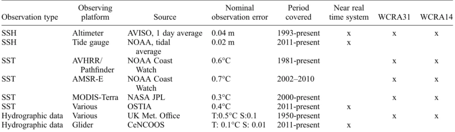
Table 1. A summary of the observation types, observing platforms, data sources, the nominal measurement errors, and the period covered for the US West Coast (WC) data assimilative simulations (WC Reanalyses, WCRA). They comprise satellite SST from multiple platforms, satellite-derived SSH, and in-situ hydrographic observations from all available platforms (including Argo proﬁling ﬂoats) in the EN3 quality controlled data base of Ingleby and Huddleston (2007) that fall within this domain.

Observation type Observing platform Source Nominal observation error Period covered Near real

time system WCRA31 WCRA14

SSH Altimeter AVISO, 1 day average 0.04 m 1993-present x x x

SSH Tide gauge NOAA, tidal

average 0.02 m 2011-present x SST AVHRR/ Pathﬁnder NOAA Coast Watch 0.6°C 1981-present x x

SST AMSR-E NOAA Coast

Watch

0.7°C 2002–2010 x x

SST MODIS-Terra NASA JPL 0.3°C 2000-present x x

SST Various OSTIA 0.4°C 2011-present x

Hydrographic data Various UK Met. Ofﬁce T:0.5°C S:0.1 1950-present x x

Hydrographic data Glider CeNCOOS T: 0.1°C S: 0.01 2011-present x

(10)

Observations assimilated during each sequence of ana-lyses were taken from a variety of platforms and are sum-marized in Table 1. To illustrate the DA impact on the CCS circulation, Figure 6(a) shows the prior model SST initial conditions on 10 February 2014, while Figure 6(b) shows the corrections made to the SST prior on the same day.Figure 6(b)reveals that the SST corrections made by 4DVAR are dominated by mesoscale features of 1°C ampli-tude.Figure 7(a)shows a time series of the total number of observations available each cycle from several platforms. For WCNRT, SSH from tide gauges is included, SST is obtained only from a gridded product, and subsurface hydrography derives only from an in-situ glider (Donlon et al. 2012).Figure 7(b) shows a time series of the ratio of posterior cost function (Jf) to the prior cost function

(Ji) for each 4DVAR from WCRA31 (WCRA14 and

WCNRT are qualitatively similar), and show that 4DVAR successfully reduces J by a factor of ~2–3 during each cycle. Figure 7(c) shows a time series of the kinetic energy from WCRA31, WCRA14 and a run of ROMS without DA forced using the prior forcing of WCRA31.

The kinetic energy is the average over the central California region between 34N and 40N from the coast to 400 km off-shore which is a region characterized by mesoscale eddy activity (Kelly et al. 1998). Figure 7(c) illustrates that both historical analyses are significantly more energetic than the forward model alone in this region, demonstrating the influence of 4DVAR on an important, largely unob-served, component of the coastal circulationfield.

Coastal-scale atmosphere-wave-ocean couplings

Oceanicflows can be strongly forced or modified by waves, in particular in the nearshore and in the coastal ocean (Longuet-Higgin 1970;Newberger & Allen 2007b;Lentz et al. 2008). Surface waves and ocean interactions control the boundary fluxes, momentum and energy exchange between the atmosphere and the ocean and within the water column. Model coupling can be achieved at different levels of complexity. A large effort has been expended to develop models capable of resolving the vertical structure of the mean flow accounting for mixing and dispersion Figure 5. Example of covariance localization in the nested Ligurian Sea ROMS model. The assimilation increment obtained from the global assimilation scheme (upper left panel), standard deviation of this increment (outer Mediterranean model, upper right panel) and the resulting localization envelope using a hypothetical observation located at the position of the marker (black circle with‘x’ symbol at 43.8N, 9.7W).

(11)

Figure 6. (a) Sea surface temperature posterior estimate on February 10, 2014 from the US West Coast Near Real Time model (WCNRT). (b) Corrections to prior model estimate of SST.

Figure 7. (a) Time series of the log10of the number of observations assimilated into the West Coast Reanalyses (WCRA) models during

each 4DVAR analysis cycle in the form of sea surface temperature (black curve), sea surface height (red curve) and in-situ hydographic data (blue curve). (b) A time series of the ratio of theﬁnal value (Jf) to the initial value (Ji) of the cost function for each 4DVAR cycle. (c) Time

series of the kinetic energy off the central California coast from WCRA31 (red curve), WCRA14 (black curve) and from a forward run of the model without data assimilation (blue curve).

(12)

keeping the hydrostatic approximation (Svendsen & Putrevu, 1994). However, a proper representation of near-surface currents and drift requires the introduction of wave effects, in particular the Stokes drift and wave-induced mixing (Rascle & Ardhuin 2009).

Main issues/challenges for couplings in the coastal ocean An important challenge in coupling coastal ocean models has been to ensure consistency in the fluxes that go between the various coupled models (atmosphere-to-ocean, atmosphere-to-wave, wave-to-(atmosphere-to-ocean, etc.). In the uncoupled paradigm, models are calibrated and validated mostly in isolation, often with limited data compared to the number of modeled processes. As a result, dissipation terms are often used as tuning parameters to force a desired model behavior. In coupled modelling, these same dissipation terms become the fluxes to other models, e.g. the dissipated energy from wind wave models that feeds into the mixing of the upper ocean in bar-oclinic circulation models. This has forced the community to reassess calibration strategies when applied to coupled model systems. In the process, this has increased the need for detailed observations of processes in the model inter-face, which were previously neglected. It has also led to a revision of the parameterization of a number of these flux transfers between models (Mellor 2008; Tsagareli et al. 2010;Babanin et al. 2010).

Examples of coupled coastal systems

The role of the coupling of wave and circulation models on improving ocean forecasts is demonstrated for the German Bight region, characterized by wind-waves and strong tidal currents (Stanev et al. 2011). Processes like nonlinear feed-back between currents and waves play an important role in this area. The coupling between the wave model (WAM) and hydrodynamical model (General Estuarine Transport Model, GETM) improves the estimates of ocean state vari-ables, especially in coastal areas and estuaries (Stanev et al. 2003a;He et al. 2012). The coupling takes into consider-ation both the effect of currents on waves and the effect of waves on upper ocean dynamics (in particular on mixing and drift currents). In WAM the depth and/or current ﬁelds can be non-stationary, grid points can become dry and refraction due to spatially varying current and depth is accounted for in the quasi-stationary approach. GETM was modiﬁed to account for wave effects by introducing the depth dependent radiation stres-ses and Stokes drift. These terms were calculated from the integrated wave parameters (Mellor 2008). The gradient of the radiation stresses serves as an additional explicit wave forcing term in the momentum equations for the horizontal velocity components. The transfer of momentum by waves becomes important for the mean water level setup and for

the alongshore currents generated by waves in the surf zone.

The role of coupling is demonstrated by analyzing the impact of waves on extreme events (storm Xavier,Figure 8). The radiation stress increases the average water levels, a pronounced effect in the coastal area. During normal con-ditions, the differences of the sea level due to the coupling with the wave model are maximum 10–15 cm around the Elbe estuary. However, during the storm, the differences of simulated sea level when considering waves are about 30–40 cm along the whole German coast. Therefore, the uncertainties in most of the presently used models result from the nonlinear feedback between strong tidal currents and wind-waves, which can no longer be ignored in the operational oceanography, particularly in the coastal zone where its role seems to be dominant.

Several other studies demonstrate the importance of wave current coupling in the coastal regions (e.g. for the NW Meditteranean) and for the Liverpool Bay (Jordà et al. 2007; Bolaños et al. 2011; Brown et al. 2011). In the framework of MyOcean European project http:// Myocean.eu, a growing effort has been devoted to wave and primitive equation models coupled in regional systems. For instance, in the Mediterranean Forecasting System (MFS) the wave and ocean models are tightly coupled to improve the representation and forecast of wave parameters and the oceanic meanﬂow (Oddo et al. 2009). The coupled (WW3-NEMO) operational MFS improves the already good results achieved by the stand-alone wave model and primitive equation model, and is able to provide the large scale information needed for the nested coastal systems. Similar efforts in the US are through NOAA’s Integrated Ocean Observing System [IOOS;http://www.ioos.noaa.gov/].

Another recent effort is based on deploying a fully coupled ocean/air/wave modelling system within the Earth System Modelling Framework (ESMF) to complete the US Navy’s COAMPS, a globally relocatable modelling system designed for operational time (days) and space (~1– 10 km) scales (Allard et al. 2014). Test cases with the wave model component are being completed as theﬁnal phase of transition to operations. Such systems can enhance existing regional models by elucidating mechanisms that may be missing or not properly accounted for in local coastal fore-casting systems. COAMPS has been deployed recently for island regions with steep terrain to elucidate the mechan-isms of wind-induced oceanic eddy formation and detach-ment in the Philippines (Pullen et al. 2008; Pullen et al. 2011; May et al. 2011; Rypina et al. 2010). In a similar vein, the air-sea coupled model has been applied to the island of Madeira. A real-time forecasting system http:// wakes.uma.pt consisting of high-resolution MM5 (now WRF) and ROMS has been operational since 2007. But such a one-way coupled system was unable to reproduce the warm wake effect whereby the cloud-free region in Journal of Operational Oceanography s157

(13)

the lee of the island leads to enhanced ocean temperatures (Sachsperger 2012; Caldeira & Tome 2013). A recent application of the two-way coupled air/sea COAMPS system is able to capture the evolution of the warm wake in the lee of Madeira in both the upper ocean and lower atmospheric boundary layer.

Coastal ecosystem response to the physical drivers The coastal and shelf seas are among the world’s most diverse and productive environments and an important component of the marine environment, accounting for up to 30 % of the ocean’s primary production, hosting major ﬁsheries of the world, and may be important in global carbon budgets (Gattuso et al. 1998;Smith & Hollibaugh 1993; Longhurst et al. 1995; Edwards et al. 2012; Pauly & Christensen 1995; Pauly et al. 2002;Holt et al. 2009). These factors pose urgent needs for expanding beyond the forecasting of physical variables.

Biogeochemical prediction in the coastal seas

Better understanding of the state of shelf sea ecosystems requires the implementation of coupled hydrodynamic and ecosystem models at regional/coastal high-resolution scales. Uncoupled ecosystem models have been developed for a wide range of applications: (a) process-oriented studies on shelf seas biogeochemical cycles, nutrient ﬂuxes and pathways; (b) understanding of the effects of eutrophication; (c) hypoxia; (d) harmful algal blooms (HABs), etc. (Proctor et al. 2003; Nobre et al. 2005; Yakushev et al. 2007; Russo et al. 2009; McGillicuddy, 2010). Coupled three-dimensional hydrodynamic-ecosys-tem models are able to simulate the biogeochemistry of coastal ecosystems but they can also advance knowledge on the ecosystem functioning (Moll & Radach 2003). Several coupled model systems have helped establish the

critical climatological, seasonal and interannual aspects of ecosystem variability, while also used to explore alternate states under different management scenarios (Hofmann & Lascara 1998;Crise et al. 1999;Brown et al. 2013; Dab-rowski et al. 2014; Wild-Allen et al. 2010; Holt et al. 2012). Coupled model systems help address the variability of the marine ecosystems and their response to the variabil-ity of physical forcing. Ventilation processes and circula-tion overturning determine the supply of waters with nutrients and support primary production. In favorable wind conditions, the upwelling in coastal areas due to Ekman transport is a mechanism providing nutrient rich waters at the surface and favoring primary production. Changes in the ocean circulation and stratiﬁcation trigger the changes of the mixed layer depth and consequently of the nutrient levels at the ocean which also has a response to the primary production (Sarmiento et al. 2004).

The winter convection triggered by air-sea exchange is also an important process for the physical impact on the ecosystem (Stanev et al. 2003b). Convective mixing is also highly influenced by the changes of the thermocline and halocline, and hence, changing the amount of nutrient available for phytoplankton growth. Another important physical driver is the freshwater river input that influences both stratification and the coastal circulation. Examples include the US west coast, the US east coast, the northern Gulf of Mexico, the Western South Atlantic shelf, the greater Caribbean, the Adriatic and Aegean Seas and the north-western Black Sea, to name a few (Kourafalou et al. 1996; Kourafalou 2001; Hu et al. 2004; Soares et al. 2007;Tsiaras et al. 2008;Hickey et al. 2010; Androu-lidakis & Kourafalou 2013). The combination of physical and biogeochemical modelling is also important when addressing connectivity between ocean and coastal areas and among remote coastal ecosystems. Such phenomena are crucial for the understanding populations (as in coral reef habitats (Sponaugle et al. 2012)), the design of Figure 8. Sea surface elevation (SLE) difference between coupled wave-circulation model (WAM-GETM) and the pure circulation model (GETM) for the German Bight on 3 December 2013 (left) and during the storm Xavier on 6 December 2013 (right).

(14)

Marine Protected Areas and the management of the world’s ﬁsheries.

Finally, the contribution of benthic nutrientﬂuxes to the total nutrient pool available for primary production uptake increases, as water depth decreases approaching the coast. Sediment layers in biogeochemical models, where reminer-alisation of nutrients and exchange with the overlying water column occurs, become increasingly important. This also forms the backbone for modelling sediment transport, which is a separate discipline delivering speciﬁc products to end users (e.g. deposition and re-suspension maps, sedi-mentation rate, fate of dredging activities).

Examples of coastal interdisciplinary systems

The interest in combined physical, chemical and biological operational products, including near-real time and forecast is increasing. Internationally implemented marine policies, aimed at protecting the sea from increasing environmental pressures, have shown the need for monitoring marine systems. In the European Union, the Water Framework Directive and the Marine Strategy Framework Directive (MSFD) are dealing with an evaluation and monitoring of the ecological status of their river basins/coastal waters and marine waters (Borja et al. 2006). Additionally, the European Marine Ecosystem Observatory EMECO, www.emeco-group.org was formed in response to new challenges posed by the MSFD and the implicit need to deliver an ecosystem-based management approach. The IOOS national network of Regional Coastal Ocean Observ-ing Systems (RCOOS) in the US has implemented bio-physical forecasts to satisfy national needs (Kourafalou et al. 2015). However, ecosystem modelling remains a highly complex and challenging task. Biogeochemical models are built on many assumptions and often empiri-cal-based parameterizations; identifying an appropriate set of parameters through trial runs is seldom straightfor-ward (Marta-Almeida et al. 2012). The strong dependency of biology on physical drivers also requires reliable near-real time coastal ocean circulation forecasts.

The coupled hydrodynamic-ecosystem model by the UK’s Met Ofﬁce provides forecasts from the Medium-Res-olution Continental Shelf POLCOMS-ERSEM system to the 7 km Atlantic Margin Model NEMO-ERSEM system (Siddorn et al. 2007). The ecosystem components in the operational system are also validated against available in-situ, satellite and climatological data. Other regions in Europe with operational modelling products for biology (all available through http://www.myocean.eu/) are the Baltic Sea and the Mediterranean Sea, with Eastern (POSEIDON) and Western basin sub-systems (Neumann 2000; Nittis et al. 2001; Borja et al. 2006; Lazzari et al. 2010).

A more extensive example is provided for the Black Sea (Figure 9), the world’s largest marine anoxic basin

(Murray et al. 1989). Anoxic conditions formed about 8,000 years ago following the reconnection of the Mediter-ranean and Black Seas and the resulting intrusion of saltier Mediterranean water (Deuser 1974). The vertical structure is represented by an oxygenated surface layer and a sulﬁde containing deep layer, separated by the suboxic zone (Murray et al. 1989;Murray et al. 1995)

The deployment of two ARGO floats in the northern Black Sea in 2010 enabled, for the first time, more than 2-year continuous observations (Figure 9). The Navigating European Marine Observer (NEMO) profilers were equipped with temperature, salinity and oxygen sensors (see trajectories in Figure 9) (Stanev et al. 2013). As the two floats operated in two dynamically very different areas, the open ocean and the coastal zone, it was a unique opportunity to compare synchronously the ences between changes of hydro-chemistry in these differ-ent zones and to evaluate biophysical model predictive capabilities. The coastalfloat NEMO-0145 revealed vigor-ous changes of oxygen, manifesting the importance of the mesoscale processes for the oxygen change. The observed oxygen variability gave clear indication that its distribution was a function of the general circulation characterized by an upward motion in the basin interior and sinking in the areas of coastal anticyclones. Extremely low temperature, as well as high oxygen concentrations, caused by the abnor-mally cold winter, persisted along the southern coast (Feb-ruary–July 2012). The correlation between time versus depth oxygen and temperature diagrams demonstrated that mesoscale eddies contributed largely to the variations of oxygen (Stanev et al. 2013).

A model-to-data comparison in the temporal variability of the upper layer oxygen is illustrated through the oxygen versus temperature relationships (Figure 9). These proﬁles are characterized by almost vertical curves in the late fall and beginning of winter, i.e. with a relatively homogeneous oxygen distribution in the cold season. The lowest oxygen values at sea surface approached 250μM both in the model and observations. The warming of surface waters was accompanied by a decrease in the surface-oxygen concen-tration and the formation of oxygen subsurface maximum. This excluded the possibility that subsurface oxygen maximum was just a direct result of oxygen-rich water created by winter convection that remained overlaid in summer by low oxygen surface water (because of the high SST). The model was thus able to replicate almost all observed features of the oxygen dynamics, making it a useful tool for investigating the upper-ocean hydrochemis-try of the Black Sea.

Utility of coastal systems

The combination of coastal ocean observations and models provides a powerful tool for describing and understanding complex ocean system interactions. By combining Journal of Operational Oceanography s159

(15)

science-based observations with well-constructed models, advances can be made toward understanding complex coastal ocean systems and development of useful tools for

managing coastal ocean resources. Applications are closely linked to the science foundation behind the physical drivers, giving feedback that provides exciting new scientific Figure 9. (Top): Black Sea topography andfloat trajectories. Locations of Argo floats surfacing are shown with yellow (NEMO-0144) and red (NEMO-0145). Deployment positions are marked by crosses, the last positions are labeled by stars. Squares in different colors show the observed positions where historical data have been analyzed. (Middle) Time versus depth plots of (a) oxygen and (b) temperature as observed by the coastal Argofloat NEMO-0145. (Bottom) Model to data comparison using oxygen versus temperature plots in location ‘A’ for the four seasons: (a) observational seasonal profiles from the coastal Argo float (NEMO-0145) data and (b) simulated seasonal pro-files from the 3D biophysical model.

(16)

challenges. Their fundamental utility is addressing broad societal and economic benefits and needs; examples follow. The Central and Northern California Coastal Ocean Observing System (CeNCOOS) is supported by both the near real-time analyses and historical analyses (outputs available at http://oceanmodelling.ucsc.edu/; http://www. cencoos.org/). Like other regional observatories, CeNCOOS provides ocean information for effective agement of coastal waters, such as ecosystem-based man-agement of marine fisheries, understanding impacts of climate change, and assessing coastal water quality issues such as Harmful Algal Blooms. Among current users of the ROMS CCS 4DVAR analyses described in the previous section are fisheries scientists whose goals are to relate oceanographic conditions with larval survival and recruit-ment data for commercially-relevant fisheries on the US west coast.

Understanding processes in coastal ocean ecology that can improve biophysical predictions and aid the manage-ment of coastal resources is another application of interdis-ciplinary coastal systems. A recent example is from the West Florida Shelf. Observations of velocity from moor-ings, water properties from glider transects, satellite imagery and K. brevis cell counts were combined with model simulations from the WFCOM (see previous section) to explain why there was no red tide on the west Florida shelf in 2010 (Weisberg et al. 2014a). It was con-cluded that both the physics of the circulation and the biology of the organism are necessary conditions for a K. brevis bloom to occur, but neither alone are sufficient conditions. In another study that similarly combined multi-disciplinary observations with model simulations, the con-undrum of how grouper larvae get from offshore adult spawning to near shore juvenile settlement sites was addressed (Weisberg et al. 2014b). Another study deals with connectivity patterns, important for understanding coral fish replenishment and aiding the management of reef resources. A high resolution biophysical model around the Southwest Florida Shelf and the Florida Keys was used, in tandem with detailed observations for model evaluation and calibration, to construct connectivity matrices for coralfish larvae (Sponaugle et al. 2012).

Maritime Domain Awareness (MDA) has beneﬁtted from an infusion of tools and technologies, and has been an active area of planning and policy in the homeland security enterprise. Partnerships and data integration are an increasingly important aspect of maritime security and law enforcement mission areas, including illegal ﬁshing interdiction and search and rescue. Linking coastal fore-casts to search and rescue decision support tools is an effec-tive strategy to reduce search times and better allocate ships and airborne assets (Breivik et al. 2013). For instance, the US Coast Guard is increasingly focused on domains such as the Arctic and island environments, where they must be able to carry out their traditional missions in challenging

conditions. Saving time and resources in such environ-ments is extremely important. The use of coastal forecast-ing for Coast Guard missions will provide even more beneﬁts in harsh operating environments where obser-vations may be limited and coastal forecasts can contribute vital situational information.

An operational search and rescue (SAR) modelling system has been developed to forecast the tracks of victims or debris from marine accidents in the marginal seas of the northwestern Paciﬁc Ocean (Cho et al. 2014). The SAR system is directly linked to a real-time operational forecasting system that provides 72 h wind and surface current forecasts for the Yellow Sea and the East and South China Seas, capable of predicting the tracks and area to be searched. The SAR modelling system is used operationally to support the Korea Coast Guard during marine emergencies. Such applications often extend to ship routing operations. While the use of weather forecast data (wind and waves) in the optimization of ship routing is more common, the incorporation of surface current infor-mation is still a challenge (Panigrahi et al. 2012;Lin et al. 2013). Focusing on the Kuroshio region, the impact of using the current or avoiding it (when travelling in the opposite direction) for reducing the transit time of ships has been demonstrated (Chang et al. 2013). For instance, using a combination of weather and ocean simulations for the Osaka Bay region (Japan), a case study evaluates the effectiveness of each forcing for optimizing the ship route (Chen et al. 2013).

As ports compete for business, shipping and cruise lines assume the responsibility of added security, and high value waterfront assets require protection, MDA approaches and solutions will continue to expand in both the public and the private sectors. With the advent of tech-nologies and procedures focused on maritime security, there is a strong role for coastal forecasting modelling to contribute to optimal performance of these security and safety-focused systems. For instance, sensor networks require information on the current and projected environ-mental operating conditions in order to estimate perform-ance characteristics. Acoustic monitors for underwater and surface threat detection (small vessels, scuba divers, small submarines, etc.) use sound propagation to detect targets. Linking coastal forecasts of temperature and sal-inity to transmission loss models can produce detailed maps of where targets could hide or detection systems should be augmented. In addition, detection systems are increasingly complex with components consisting of acoustic sensors, radar, and cameras (Pullen & Bruno 2014). In order to promote optimal performance, sensors need to be able to cue each other to examine targets or turn on/off during different operating conditions so that the best performing sensor, given the particular coastal con-ditions, is operating. This paradigm represents a smart implementation of sensors joined with high-resolution, Journal of Operational Oceanography s161

(17)

accurate coastal forecasts and suggests another way in which coastal ocean forecasting can enhance maritime domain awareness.

Modelling the transport and fate of hydrocarbons resulting from oil spills is another example of the utility of coastal prediction systems. The major 2010 oil spill acci-dent from the Macondo well in the Gulf of Mexico has attracted a large number of efforts to improve predictive capabilities in a complex regional sea, which is subject to intense ocean exploration form the oil and gas industries. Several immediate applications were made at the time of the spill (Mezic et al. 2010; Liu et al. 2011; Mariano et al. 2011; Weisberg et al. 2011). Subsequent analyses expand on the need for downscaling to improve the inter-actions between basin-wide (i.e. the Gulf Stream) and coastal currents (i.e. wind-driven and buoyancy-driven cur-rents and intense slope exchanges) for tracking the oil and exploring its environmental consequences (Paris et al. 2012;Le Hénaff et al. 2012;Kourafalou et al. 2013; Weis-berg et al. 2014c). Two of the main uses of operational ocean numerical modelling are monitoring and forecasting of marine pollution and impacts of offshore activities (Hackett et al. 2009).

The complexity of the oil tracking models and their dependence on the oceanic and atmospheric forecasts has also been shown (Marta-Almeida et al. 2013b). European operational models are being extended with the ability to predict the behavior and evolution of an oil spill in the marine environment and linking it to an online risk assess-ment/contingency response tool available for stakeholders (Janeiro et al. 2012). Within the IONIO (Ionian integrated Marine Observatory, www.ionioproject.eu) project, in support of coastal management, a Pollution Hazard Mapping Decision Support System has been developed. Hazard mapping (Figure 10) appears as the most appropri-ate way to approach the management of oil pollution in marine areas in order to sustain the ecosystem health

state. The methodology integrates the ship trafﬁc data with the data on currents and temperature from the Oper-ational Modelling System together with the fate and trans-port oil spill model (MEDSLIK-II) (De Dominicis et al. 2013).

Coastal wave and storm surge modelling has signiﬁcant beneﬁts to coastal communities. These communities are increasingly vulnerable to powerful land falling hurricanes and extra-tropical storms, and need guidance on how to prepare for, and respond to water-related calamities. In the US, operational guidance from storm surge and inunda-tion models such as the SLOSH-based P-Surge and the ADCIRC-based ESTOFS are used to inform emergency managers on whether or not to evacuate coastal regions ahead of storm events (Feyen et al. 2013). Similar models are applied in hindcast mode to assess risks in hurricane preparedness and insurance studies.

In itself, detailed nearshore wave guidance, provided in the US by NOAA’s Nearshore Wave Prediction System (NWPS), has a number of applications in the commercial and recreational coastal waters. Accurate forecasts of wave conditions in coastal regions and in entrance channels and inlets, especially under the inﬂuence of steepening cur-rents, are critical to safety of life at sea. In terms of rec-reational activities, the leading cause of beach drowning in the US is rip currents. An operational rip current prediction system has been successfully prototyped within NWPS, showing high skill compared to recorded rip current sightings (Dusek & Seim 2013; Dusek et al. 2014).

Conclusions

Advancement of forecasting in coastal and shelf seas requires continuous development of innovative method-ologies and tools, in support of research and applications. The magnitude of the sampling problem and the short Figure 10. Monthly averaged surface oil hazard maps (> 1 kg/km2probability of oil presence) in the southern Adriatic Sea (left panel) and ship line distribution (right panel) over the same area during June 2012.

(18)

space and time scales preclude ever having enough obser-vations to fully describe the coastal ocean. Coastal Ocean Forecasting Systems (COFS) that integrate observatories with models are thus required, working in synergy to assess and predict coastal phenomena of interest and satisfy the needs of well-deﬁned users. Within GODAE OceanView, the COSS-TT promotes international collabor-ation in addressing all scientiﬁc issues related to COFS needs and downstream applications, aiming to promote a seamless framework of observations and data assimilative models from the global to the coastal/littoral scale.

Coastal ocean models in COFS require dedicated numerical techniques for both individual ocean com-ponents and fully coupled models. A primary science topic is downscaling from larger scale models, toward the development of appropriate nesting procedures. These include assessment of the boundary conditions provided to COFS nested systems from larger scale systems, and reﬁnement of model set-up (including grids, topographic details and forcings). Other primary topics driving COFS research and development were discussed, especially issues associated with model coupling and data assimila-tion in the coastal ocean, including assessment of model errors. A challenge for coupling is to ensure consistency in theﬂuxes between the modelling components. For data assimilation, challenges arise due to the relative importance of the boundary conditions compared to the initial con-ditions, and due to anisotropic processes in the coastal zone. It was highlighted that the above physical drivers have a pronounced impact on coastal ecosystem function-ing and connectivity among remote ecosystems.

Benefits from scientific and technical advances associ-ated with COFS encompass a wide range of socioeconomic aspects. These include: environmental studies required for permits and oversight for the management of marine resources, construction, oil/gas exploration, insurance claims etc.; sea treaties and agreements (regulation of natural resources, marine pollution litigation, regionalfish stock management, Marine Protected Areas, United Nations Convention on the Law of the Sea/UNCLOS, etc.); recreational and commercial fishing; search and rescue; Maritime Domain Awareness; mitigation of natural disasters, climate change and extreme events; pre-dictions on the transport and fate of pollutants. Advance-ments in COFS will further develop consistent protocols for observation impact assessment, tools for routine pro-duction of appropriate diagnostics, common sets of metrics for inter-comparison of results, and objective meth-odologies for observing system design and assessment activities.

Acknowledgements

V. Kourafalou acknowledges NOAA support (NA13OAR 4830224 and NA12OAR4310073) and H. Kang (UM/RSMAS)

for help with manuscript formatting. P. De Mey and N. Ayoub have closely collaborated with P. Marsaleix (CNRS/LA, France) and have been supported from CNES through the Ocean Surface Topography/Jason project MICSS and from CNRS/ INSU. A. Barth was supported in part by the National Fund for Scientiﬁc Research, Belgium (F.R.S.-FNRS) and the SANGOMA project (FP7-SPACE-2011-1-CT-283580-SANGOMA). The research by Y. Chao was supported by NOAA/IOOS (through CeNCOOS, SCCOOS) and the NASA Interdisciplinary Science program. M. Herzfeld is thankful to the eReefs marine modelling team and partners (CSIRO: Com-monwealth Industrial and Scientiﬁc Research Organization; SIEF: Science and Industry Endowment Fund; AIMS: Australian Institute of Marine Science). A. Moore acknowledges support from the US National Science Foundation (OCE 1061434) and by NOAA/IOOS through CeNCOOS. R.H. Weisberg was assisted by L. Zheng and both were supported in part by the BP/The Gulf of Mexico Research Initiative through the Deep-C Program hosted at the Florida State University.

References

Allard R, Rogers E, Martin P, Jensen T, Chu P, Campbell T, Dykes J, Smith T, Choi J, Gravois U. 2014. The US Navy Coupled Ocean-Wave Prediction System. Oceanography. 27(3): 92– 103,http://dx.doi.org/10.5670/oceanog.2014.71

Androulidakis YS, Kourafalou VH. 2013. On the processes that influence the transport and fate of Mississippi waters under flooding outflow conditions. Ocean Dyn. 63(2–3): 143–164. Auclair F, Marsaleix P, De Mey P. 2003. Space-time structure and dynamics of the forecast error in a coastal circulation model of the Gulf of Lions. Dyna Atmos Oceans 36: 309–346,doi:10. 1016/S0377-0265(02)00068-4.

Auclair F, Marsaleix P, Estourne C. 2001. The penetration of the Northern Current over the Gulf of Lions (Mediterranean) as a downscaling problem. Oceanol Acta. 24(6): 529–544. Babanin AV, Tsagareli KN, Young IR, Walker DJ. 2010.

Numerical Investigation of Spectral Evolution of Wind Waves. Part II: Dissipation Term and Evolution Tests. J Phy Oceanogr. 40: 667–683.

Barth A, Alvera-Azcárate A, Beckers J-M, Rixen M, Vandenbulcke L. 2007. Multigrid state vector for data assim-ilation in a two-way nested model of the Ligurian Sea. J Mar Syst. 65: 41–59,doi:10.1016/j.jmarsys.2005.07.006. Bennett AF. 2002. Inverse Modelling of the Ocean and

Atmosphere. Cambridge, University Press, 234pp.

Blumberg AF, Kantha LF. 1985. Open boundary condition for cir-culation models. J Hydraul Eng. 111: 237–255.

Bolaños R, Osuna P, Wolf J, Monbaliu J, Sanchez-Arcilla A. 2011. Development of the POLCOMS–WAM current–wave model. Ocean Model. 36(1–2): 102–115.

Borja and co-authors.. 2006. The European Water Framework Directive and the DPSIR, a methodological approach to assess the risk of failing to achieve good ecological status. Estuarine, Coastal and Shelf Science 66: 84–96.

Breivik Ø, Allen AA, Maisondieu C, Olagnon M. 2013. Advances in Search and Rescue at Sea. Ocean Dyn. 63: 83–88,doi:10. 1007/s10236-012-0581-1.

Brinkman RM, Wolanski EJ, Deleersnijder E, McAllister FA, Skirving WJ. 2002. Oceanic inﬂow from the Coral Sea into the Great Barrier Reef. Estuarine Coastal and Shelf Science 54: 655–668.

Brown CW, Hood RR, Long W, Jacobs J, Ramers DL, Wazniak C, Wiggert JD, Wood R, Xu J. 2013. Ecological forecasting in Journal of Operational Oceanography s163

(19)

Chesapeake Bay: Using a mechanistic–empirical modelling approach. J Mar Syst. 125: 113–125.

Brown J, Bolaño R, Wolf J. 2011. Impact assessment of advanced coupling features in a tide–surge–wave model, POLCOMS-WAM, in a shallow water application. J Mar Syst. 87(1): 13–24.

Burrage DM, Church JA, Steinberg CR. 1991. Linear systems analysis of Momentum on the continental shelf and slope of the Central Great Barrier Reef. J Geophys Res. 96(C12): 22169–22190.

Cailleau S, Fedorenko V, Barnier B, Blayo E, Debreu L. 2008. Comparison of different numerical methods used to handle the open boundary of a regional ocean circulation model of the Bay of Biscay. Ocean Model. 25: 1–16.

Caldeira R, Tome R. 2013. Wake Response to an Ocean-Feedback Mechanism: Madeira Island Case Study. Bound-Lay Meteorol. 148(2): 419–436.

Chang Y-C, Tseng R-S, Chen G-Y, Chu P C, Shen Y-T. 2013. Ship Routing Utilizing Strong Ocean Currents. The Journal of Navigation 66: 825–835.

Chao Y, Li Z, Farrara J, McWilliams C, Bellingham J, Capet X, Chavez F, Choi J-K, Davis R, Doyle J, et al. 2009. Development, implementation and evaluation of a data-assimilative ocean forecasting system off the central California coast. Deep-Sea Res II. 56: 100–126.

Chao Y, Li Z, Farrara JD, Moline MA, Schoﬁeld OME, Majumdar SJ. 2008. Synergistic applications of autonomous underwater vehicles and the regional ocean modelling system in coastal ocean forecasting. Limnol Oceanogr. 53: 2251–2263.

Chassignet EP, Hurlburt HE, Metzger EJ, Smedstad OM, Cummings J, Halliwell GR, Bleck R, Baraille R, Wallcraft AJ, Lozano C, Tolman H, Srinivasan A, Hankin S, Cornillon P, Weisberg R, Barth A, He R, Werner C, Wilkin J. 2009. U.S. GODAE: Global Ocean Prediction with the HYbrid Coordinate Ocean Model (HYCOM). Oceanography 22: 48–59.

Chen C, Shiotani S, Sasa K. 2013. Numerical ship navigation based on weather and ocean simulation. Ocean Eng. 69: 44–53.

Chen CS, Liu H, Breadsley RC. 2003. An unstructured, ﬁnite-volume, three-dimensional, primitive equation ocean model: application to coastal ocean and estuaries. J Atmos Ocean Tech. 20: 159–186.

Cho K-H, Li Y, Wang H, Park K-S, Choi J-Y, Shin K-I, Kwon J-I. 2014. Development and Validation of an Operational Search and Rescue Modelling System for the Yellow Sea and the East and South China Seas. J Atmos Ocean Tech. 31: 197–215.

Crise and co-authors.. 1999. The Mediterranean pelagic ecosys-tem response to physical forcing. Prog Oceanogr. 44: 219– 243.

Dabrowski T, Lyons K, Berry A, Cusack C, Nolan G D. 2014. An operational biogeochemical model of the North-East Atlantic: Model description and skill assessment. J Mar Syst. 129: 350– 367.

De Dominicis M, Pinardi N, Zodiatis G, Archetti R. 2013. MEDSLIK-II, a Lagrangian marine surface oil spill model for short-term forecasting - Part 2: Numerical simulations and validations. Geoscientiﬁc Model Developmen 6: 1871– 1888,doi:10.5194/gmd-6-1871-2013.

De Mey P and co-authors.. 2009. Applications in Coastal Modelling and Forecasting. Oceanography 22(3): 198–205. Debreu L, Blayo E. 2008. Two-way embedding algorithms: a

review. Ocean Dyn. 58: 415–428.

Debreu L, Marchesiello P, Penven P, Cambon G. 2012. Two-way nesting in split-explicit ocean models: Algorithms, implemen-tation and validation. Ocean Model. 49–50: 1–21.

Deuser WG. 1974. Evolution of anoxic of anoxic conditions in the Black Sea during Holocene. The Black Sea-Geology, Chemistry and Biology 2: 133–136.

Dobricic S, Pinardi N, Adani M, Tonani M, Fratianni C, Bonazzi A, Fernandez V. 2007. Daily oceanographic analyses by Mediterranean Forecasting System at the basin scale. Ocean Sci. 3: 149–157.

Dombrowsky E, Bertino L, Brassington GB, Chassignet EP, Davidson F, Hurlburt HE, Kamachi M, Lee T, Martin MJ, Mei S, Tonani M. 2009. GODAE systems in operation. Oceanography 22(3): 80–95.

Donlon CJ, Martin M, Stark JD, Roberts-Jones J, Fiedler E, Wimmer W. 2012. The Operational Sea Surface Temperature and Sea Ice analysis (OSTIA). Remote Sens Environ.doi:10.1016/j.rse.2010.10.017.

Doyle JD, Jiang Q, Chao Y, Farrara J. 2009. High-resolution real-time modelling of the marine atmospheric boundary layer in support of the AOSNII ﬁeld campaign. Deep-Sea Res II. 56: 87–99.

Dusek G, Seim H. 2013. A probabilistic rip current forecast model. J Coastal Res. 29(4): 909–925.

Dusek G, van der Westhuysen AJ, Gibbs A, King D, Kennedy S, Padilla R, Seim H, Elder D. 2014. Coupling a Rip Current Forecast Model to the Nearshore Wave Prediction System. To appear in Proc. 94rd AMS Annual Meeting, Atlanta, GA. Edwards P, Barciela R, Butensch M. 2012. Validation of the NEMO-ERSEM operational ecosystem model for the North West European Continental Shelf. Ocean Sci. 8: 983– 1000. www.ocean-sci.net/8/983/2012/doi:10.5194/os-8-983-2012.

Errico RM, Vukićević T. 1992. Sensitivity analysis using an adjoint of the PSU–NCAR mesoscale model. Mon Weather Rev. 120: 1644–1660.

Evensen G. 2003. The Ensemble Kalman Filter: theoretical for-mulation and practical implementation. Ocean Dyn. 53: 343–367,doi:10.1007/s10236-003-0036-9.

Feyen JC, Funakoshi Y, van der Westhuysen AJ, Earle S, Caruso Magee C, Tolman HL, Aikman FIII. 2013. Establishing a Community-Based Extratropical Storm Surge and Tide Model for NOAA’s Operational Forecasts for the Atlantic and Gulf Coasts. Proc. 93rd AMS Annual Meeting, Austin, TX.

Flather RA. 1988. A numerical investigation of tides and diurnal-period continental shelf waves along Vancouver Island. J Phys Oceanogr. 18: 115–139.

Frankignoulle M, Bourge I, Romaine S, Buddemeier RW. 1998. Effect of calcium carbonate saturation of sea-water on coral calciﬁcation. Global and Planetary Change 18: 37–46,

doi:10.1016/S0921-8181(98)00035-6.

Gattuso J-P and co-authors. 1998. Seawater carbonate chemistry and calciﬁcation rate of colonies of Stylophora pistillat.

doi:10.1594/PANGAEA.761768, Supplement to: Gattuso JP;. Guillou N, Chapalain G, Duvieilbourg E. 2013. Sea surface temp-erature modelling in the Sea of Iroise: assessment of boundary conditions. Ocean Dyn. 63(7): 849–863.

Hackett B, Comerma E, Daniel P, Ichikawa H. 2009. Marine oil pollution prediction. Oceanography 22: 168–175.

Hamill TM, Whitaker JS, Snyder C. 2001. Distance-dependent ﬁl-tering of background error covariance estimates in an ensem-ble Kalmanﬁlter. Mon Weather Rev. 129: 2776–2790. He Y, Stanev E, Yakushev E, Staneva J. 2012. Black Sea

biogeo-chemistry: Response to decadal atmospheric variability