Using survival analysis to predict the harvesting of forest
stands in Quebec, Canada
Melo, L.C.
1*, Schneider, R.
2, Manso, R.
1,3, Saucier, J-P.
4, and Fortin, M.
11
INRA/AgroParisTech, Laboratoire d’Etude des Ressources Forˆet-Bois (UMR 1092 LERFoB), 54042, Nancy, France
2Universit´e du Qu´ebec `a Rimouski - UQAR, Rimouski, Qu´ebec G5L 3A1, Canada 3Northern Research Station, Roslin, Midlothian, UK, EH25 9SY
4Minist`ere des Forˆets, de la Faune et des Parcs, Gouvernement du Qu´ebec, G1H 6R1, Canada *Corresponding author: laracmelo@gmail.com
Abstract
Survival analysis methods make better use of temporal information, accommodate multiple levels of explanatory variables, and are meant to deal with interval-censored data. In a context of harvest modeling, this approach could improve some known limi-tations. In this study, we used data from a network of permanent plots in the province of Quebec, Canada, as a real-world case study. We tested the potential of survival anal-ysis to predict plot-level harvest probabilities from plot- and regional-level variables. The approach also included random effects in order to account for spatial correlations. The results showed the potential of survival analysis to provide annual predictions of harvest occurrence. Both regional and time-varying variables, as well as spatial pat-terns, had important effects on the probability of a plot to be harvested. Respectively, reductions in the annual allowable cut volumes led to a decrease in the harvest prob-abilities. Greater harvest probabilities were associated with the broadleaved dynamics class and higher values of basal area. In contrast, they were decreased by stem density and slope classes. The spatial random effect resulted in an improvement of the model fit. Our plot-level model improved some limitations reported in previous studies by taking the effect of a time-varying regional variable into account.
Keywords: Interval-censored, Regional-level variable, Random effect, Likelihood, Harvest model, Long-term projection, Strategic planning.
1
Introduction
Understanding forest dynamics is essential to the development of long-term strategies to ensure the sustainable use of natural resources and conservation. Sustainability is closely dependent on forest management practices. The concept of sustainability has evolved to encompass a more complex understanding of the diversity of values, resources and ecological services that forests represent (Sample, 2004). For a long time, forest management plans only focused on timber production and economic concerns in many countries around the world (Dong et al., 2015). Today, forest managers address new challenges, taking environmental protection and social demands linked to economical interests into consideration (Hernandez et al., 2014). The inclusion of these new factors has led to increasingly complex decision-making procedures, which, in turn, require decision models to meet and support this new approach (Hernandez et al., 2014).
Forest management planning consists of making decisions about what to do in the future given what is known about the past and the present. This type of planning is based on a hierarchical structure that consists of both strategic and tactical decisions. The aim of the strategic level is to help with decisions related to sustainable harvests that take large areas, long-term time horizons, silvicultural policies and legislation issues into account (Martell et al., 1998). At the tactical level, the objective is to conduct harvest operations on a short-term horizon for specific areas (Martell et al., 1998). Since these strategic decisions are often the result of a modeling process for long-term horizons, we have decided to focus on this aspect.
Different methodologies have been developed to address the complex choice of which trees or plots should be harvested in long-term growth projections (Fortin, 2014). They can be grouped into two categories: harvest algorithms and harvest models. Harvest algorithms are based on user-defined rules that can be used to specify which trees should be harvested considering stand characteristics such as the diameter classes and stand basal area (e.g., Miina, 1996; Pukkala et al., 1998). Harvest algorithms generally provide optimal solutions. This optimum means considering both time and the objective function (Pukkala and Kurttila, 2005). Depending on the objective function, the application of harvest algorithms may be a difficult task. When the strategy includes uneven-aged and mixed forests, this complexity is even greater (Thurnher et al., 2011).
An alternative to harvest algorithms has been the development of statistical models that predict the tree- or plot-level probability of being harvested (e.g., Sterba et al., 2000; Thurnher et al., 2011; Ant´on-Fern´andez and Astrup, 2012; Fortin et al., 2013). These models all use logistic regressions. However, the logistic regression has some limitations in a context of harvest planning, especially when the exact date of the harvest is unknown, which is the case in many inventories. The harvest model is then fitted on time intervals bounded by two successive measurements, the first one providing the initial conditions, whereas the second one gives the information as to whether or not the plot or the tree has been harvested in the meantime. If the sampling intensity changes over time or if the intervals overlap, the maximum likelihood estimates of the model parameters may be biased (Firth, 1993; McCullagh, 2008). Additionally, uneven time intervals are an issue for the logistic regression since this technique does not effectively use temporal information (Wang et al., 2013).
methods to deal with lifetime data, which is defined as the time elapsed until the change of state of an individual (e.g., death), referred to as “event”. In our context, this event would be the harvesting of a plot or some trees in that plot. Survival analyses are especially meant to predict the probability that a harvest occurs within a given interval of time, although the exact moment is unknown. These data are commonly referred to as interval-censored data (Lawless, 2003, p. 10). As mentioned by Wang et al. (2013), survival analysis makes better use of temporal information, minimizing uncertainties in the estimation process.
Beyond the issue of interval-censored data, it is worth mentioning that the values of some potential explanatory variables may change within the time intervals, a typical issue that is known as time-varying explanatory variables and that can also be tackled using survival analysis (Allison, 1982). Time-varying variables may be richer since they provide additional information that better explain the results.
The flexibility of survival analysis methods also makes it possible to accommodate multi-ple levels of explanatory variables, which are defined at the geographic scale at which they are measured. In addition to the usual plot-level explanatory variables, regional- and national-level variables may also play a relevant role. Ant´on-Fern´andez and Astrup (2012) observed that the changes in economy or legislation were a limiting factor in their study. Likewise, Thurnher et al. (2011) also reported that changes in global management practices had con-siderable effects on predictions from harvest models. The survival analysis approach could prove to be more effective by considering the effects of variables, in contrast to the traditional logistic regression.
In forestry, some authors have already used the survival analysis approach to fit models of individual tree mortality (e.g., Rose et al., 2006; Manso et al., 2015). However, to the best of our knowledge, the survival analysis approach has not yet been applied in harvest modeling. Thus, our main objective was to test its applicability in a context of plot-level harvest occurrence. On the basis of three hypotheses, we attempted to determine whether or not survival analysis can overcome some limitations reported in the forest harvest literature. More specifically, our hypotheses were: (1) The survival analysis approach provides unbiased predictions of harvest occurrence (Hypothesis 1); (2) Regional variables have an effect on harvest occurrence (Hypothesis 2) and; (3) Time-varying covariates contribute to increasing the model likelihood (Hypothesis 3). To test these three hypotheses, we used the data from a network of permanent plots in the province of Quebec, Canada, as a real-world case study.
2
Material and methods
2.1
Dataset
The dataset we used in this study was taken from the network of permanent plots of Quebec’s Ministry of Forests, Wildlife and Parks (MFWP). This permanent plot network covered the two vegetation zones in Quebec, which also reflected major climate subdivisions: the northern temperate zone, dominated by broadleaved and mixed stands, and the boreal zone, in which coniferous stands were predominant.
The network comprised 12,570 randomly located sample plots that were established in the early 1970s to monitor forest dynamics (Fig. 1). The sampling intensity was set to one plot
every 26 km2 in the temperate zone and to one plot every 259 km2 in the boreal zone, mainly because broadleaved and mixed stands were more heterogeneous (MFFP, 2014). The plots were supposed to be measured every 10 years but, for practical reasons, the intervals between the measurements were uneven in most cases, which resulted in two to six measurements per plot. In these 400-m2 circular plots, trees with diameter at breast height (dbh: 1.3 m in
height) equal to or greater than 9.1 cm were tagged for individual monitoring. At each measurement, their diameter and status, i.e., alive, dead or harvested, were recorded.
50°W 60°W 60°W 70°W 70°W 80°W 80°W 50°N 50°N 0 750 km Permanent plots Southern part of Quebec
Figure 1: Distribution of the 12,570 permanent plots that compose the network of Quebec’s provincial forest inventory covering the northern temperate zone and the boreal zone.
Our objective was to model the harvest occurrence at the plot level. For this purpose, the measurements of the same plot were grouped into non-overlapping successive intervals. For example, if a plot had three measurements, measurements one and two were paired to create a first interval, whereas measurements two and three were used to create a second interval. In these non-overlapping successive intervals, we considered that the first measure-ment represented the initial conditions of the plot. The second measuremeasure-ment that composed the interval provided the response variable, namely whether the plot had been harvested or not and so on. A plot was considered to be harvested if at least one tree had been harvested during the interval.
Different plot-level variables were tested in the model as possible predictors of the harvest occurrence. These variables were: basal area (m2ha−1); stem density (stem ha−1); length of the interval (years); and slope class, which discriminated between accessible and non-accessible forest stands.
The ecological type, which is a classification based on the physical characteristics of the site, forest dynamics and structural elements of the vegetation (Saucier et al., 2009, p.
186-205), was also available for each plot. However, there were too many to consider them all in a model and, consequently, they were grouped into three classes based on forest dynamics: B, M and C, for broadleaved, mixed and coniferous ecological types, respectively. These forest dynamics classes actually represented the forest composition of the late successional stage. The dominant forest dynamics class was coniferous, followed by the mixed and the broadleaved classes (Boulay, 2015).
Regarding our second hypothesis on the effect of regional variables, we investigated some political and economic factors relevant to our case study. For instance, the American coun-tervailing duty on Canadian wood was a result of actions by the U.S. government to restrict Canadian lumber products since 1982 and that had a considerable impact on the harvest regime and trade in the early 2000s (Rahman and Devadoss, 2002; Descˆoteaux and Martin, 2009). The currency exchange rate could also be an important factor because it affects the profitability of Canadian lumber wood exports towards the United States. In Canada, the drop in the market in the early 2000s, with a sharp decrease in 2005, could have impacted the harvest occurrence.
At the regional level, the annual allowable cut volumes (AAC) are major drivers in forest planning in Quebec and it could be reasonably assumed that they would affect the plot-level harvest occurrence. Since 1988, Quebec’s forest law prescribes a mandatory calculation of a maximum volume that can be sustainably harvested. The allowable cut volumes are recalculated every 5 years. For further details about this calculation, the reader is referred to MFFP (2003, 2013). Regional values of AAC were retrieved from the annual reports on the state of Quebec’s forest (Parent, 1988, 1990, 1992, 1993, 1994, 1996, 1999; Parent and Fortin, 2000, 2002, 2003, 2004, 2005, 2006, 2007, 2008; Parent, 2009, 2010; Parent et al., 2012; Boulay, 2013, 2015).
This value is usually expressed as the potential in terms of cubic meters in the different administrative regions. However, since the regions do not share the same forested area, we reported these values on a hectare basis (m3ha−1). Given the anticipated incidence of the
AAC, we kept only the intervals for which this variable was available. After this screening, 12,596 intervals out of 29,013 were kept, corresponding to the 1988-2014 period. A summary of this subset is shown in Tables 1 and 2.
Table 1: Summary of some plot-level characteristics in the intervals between 1988 and 2014 for each dynamics class (B: broadleaved; M: mixed; C: coniferous; n: number of intervals; the range of the variables appears in parentheses). A particular interval belongs to a period when its final date falls into the range.
Dynamics
Period n Basal area Stem density Proportion
class (m2ha−1) (stems ha−1) harvested
B 1988-1998 296 21.8 (0.2-63.8) 599 (25-2200) 20.9% 1999-2009 1442 19.1 (1.9-45.9) 596 (25-1900) 26.6% 2010-2014 290 21.0 (0.2-45.9) 604 (25-1700) 29.0% M 1988-1998 450 18.0 (0.2-63.3) 746 (25-3575) 7.8 % 1999-2009 3623 20.8 (0.2-62.6) 793 (25-3975) 13.4% 2010-2014 1147 19.5 (0.19-62.6) 872 (25-3975) 12.2% C 1988-1998 426 16.3 (0.2-64.1) 818 (25-3050) 7.5% 1999-2009 3059 14.5 (0.2-56.3) 870 (25-3450) 10.8% 2010-2014 1863 15.2 (0.2-57.8) 881 (25-3750) 7.9%
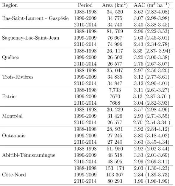
Table 2: Annual allowable cut volumes (AAC) by administrative regions since 1988. The values of AAC and area represent the mean during the period, including public and private lands.
Region Period Area (km2) AAC (m3 ha−1)
Bas-Saint-Laurent - Gasp´esie
1988-1998 34, 530 3.62 (2.82-4.08) 1999-2009 34 775 3.07 (2.98-3.98) 2010-2014 34 740 3.40 (3.38-3.45) Saguenay-Lac-Saint-Jean 1988-1998 81, 769 2.96 (2.22-3.53) 1999-2009 76 667 2.63 (2.45-3.01) 2010-2014 74 996 2.43 (2.34-2.78) Qu´ebec 1988-1998 26, 117 3.35 (2.87- 3.94) 1999-2009 26 502 3.20 (3.00-3.38) 2010-2014 26 577 2.75 (2.67-3.07) Trois-Rivi`eres 1988-1998 35, 047 2.97 (2.56-3.20) 1999-2009 34 835 3.12 (2.77-3.61) 2010-2014 34 847 3.12 (2.90-4.01) Estrie 1988-1998 7,733 3.11 (2.61-3.27) 1999-2009 7670 3.13 (2.87-3.70 ) 2010-2014 7668 3.04 (2.82-3.93) Montr´eal 1988-1998 30, 239 3.57 (2.98-4.96) 1999-2009 31 426 2.93 (2.71-3.55) 2010-2014 26 577 2.70 (2.54-3.34 ) Outaouais 1988-1998 28, 931 3.92 (2.84-4.12) 1999-2009 27 245 3.80 (3.18-4.02) 2010-2014 27 240 3.63 (3.45-4.34) Abitibi-T´emiscamingue 1988-1998 51, 950 2.92 (2.02-3.44) 1999-2009 48 518 3.33 (2.01-3.69) 2010-2014 48 595 2.99 (2.69-3.11) Cˆote-Nord 1988-1998 153, 174 2.03 (1.30-4.23) 1999-2009 103 367 2.34 (1.89-3.73) 2010-2014 80 293 1.96 (1.96-1.99)
2.2
Statistical development
The underlying concepts of the survival analysis approach are fully described in Allison (1982) and Lawless (2003). In order to illustrate the approach, let T be a non-negative random variable that represents the time at which the event of interest precisely occurred. The cumulative distribution function (cdf) given by F (t) = Pr[T ≤ t] and the probability density function (pdf) designated by f (t) are mathematical specifications of the distribution of T . Given the cdf, the survival function, which represents the probability that the event has not yet occurred at time t, can be defined as:
S(t) = Pr[T > t] = 1 − F (t) (1)
The hazard function h(t) is the instantaneous rate of occurrence at time t, provided that the event has not yet occurred, such that h(t) = f (t)S(t). Analogously, the cumulative hazard function is defined as the sum of all the hazards accumulated since the beginning of the experiment:
H(t) = Z t
0
h(z)dz. (2)
The survival function can be linked to the hazard function as follows:
S(t) = e−R0th(z)dz (3)
In the discrete case, the survival function can be alternatively defined as (e.g., Lawless, 2003, p. 10):
S(t) = e−Ptz=0h(z) (4)
There are many different formulations for hazard functions (Willet and Singer, 1993), including the proportional hazard function. This formulation assumes that some covariates increase or decrease a common hazard that is referred to as the baseline. If we define i, j, and k as the indices of the clusters of plots, plots and intervals, respectively, then a proportional hazard function can be expressed as follows:
hijk(t) = h0(t, gijkγ)exijkβ (5)
where h0 is the baseline, xijk and gijk are row vectors of explanatory variables, and γ
and β are two column vectors of unknown parameters. Note that vectors gijk and γ define the baseline, whereas vectors xijk and β define the proportional effect on the baseline. If
some covariates in gijk change within a given interval of time and their values are known for each time t, then it is possible to use these updated values in the hazard function, which is actually one method for considering time-varying covariates in the model.
Considering the context of our study, we did not know the exact time of harvest occur-rence. We only knew that a particular plot had survived until the beginning of the interval t1 and that it had been harvested or not at the end of the interval, namely at time t2. The
harvest probability is thus conditional on the survival up to the beginning of the interval. Let us define a binary variable yijk that adopts the value 1 if the plot has been harvested
during interval k in cluster i and plot j, and 0 otherwise. The probability of an occurrence during such an interval is thus given by:
Pr[yijk = 1] = Pr[t1 < T ≤ t2] = Sijk(t1) − Sijk(t2) (6)
The second issue is that we do not know the whole plot history. The main consequence of this is that actual calendar times corresponding to t1 and t2 are also unknown. This concept
is known as left-truncation (Lawless, 2003, p. 68). To take this left-truncation into account, the probability in Eq. 6 has to be conditional on the survival up to t1:
Pr[yijk = 1] = Pr[t1 < T ≤ t2|T > t1] =
Sijk(t1) − Sijk(t2)
Sijk(t1)
(7) Incorporating the hazard function 5 into Eq. 7 yields:
Pr[yijk = 1] = 1 − e−Pt2z=0h(z) e−Pt1 z=0h(z) = 1 − eexijkβ−Pt2z=t1h0(z,gijkγ) ≡ f (x ijk, gijk, β, γ) (8)
The likelihood of the parameters with respect to the whole dataset will then be:
L(β, γ | X, G, y) = Y i Y j Y k f (xijk, gijk, β, γ) yijk(1 − f (x ijk, gijk, β, γ)) 1−yijk (9)
where the rows of X, G and y contain the xijk, gijkand yijk, respectively. All parameters
can be estimated by maximizing the likelihood function with respect to γ and β.
It could be reasonably assumed that spatial correlation existed in the plot-level occurrence of harvest. These spatial correlations were treated as random effects on the baseline. Some preliminary analyses showed that the harvest occurrence was positively correlated in space and it could be reasonably assumed that these correlations decreased with increasing distances between two plots. To assess the correlation pattern, we first defined plot clusters at different scales.
These clusters were set according to the hierarchical mapping system in Quebec, which is actually composed of four nested grids of different resolutions. One grid square covered approximately 256,000 km2, 16,000 km2, 1,000 km2and 250 km2, depending on the resolution of the grid. Those squares defined by the different grids are referred to as map elements and we used the indices 1 to 4 for the highest to the lowest resolution.
The cruise line could be interpreted as a fifth resolution, representing a local scale. It referred to a straight line transverse to a slope in which data are collected. According to the sampling design, it was established to contain two plots separated by 425 m. The approximate area represented by a cruise line was 0.57 km2, which actually represented the highest resolution. Cruise line and map elements at the different scales were successively tested in the model baseline as grouping factors for cluster random effects.
From a statistical perspective, the specification of random effects in the model makes the parameter estimation more complex. Function 8 has to be redefined as f (xijk, gijk, β, γ, ui)
likelihood has to be marginalized over the distribution of the random effects. We omit the mathematical developments, but the reader is referred to Pinheiro and Bates (2000, p. 62) for further details about the estimation. Such marginal likelihood functions can be optimized using the NLMIXED procedure available in SAS (SAS, 2015, Ch. 82). An example of the implementation of this type of model is shown in Appendix A.
2.3
Model evaluation
The evaluation of the models was carried out taking variable significance and the Akaike Information Criterion (AIC) into account. Once the model is fitted, the expectation of the harvest probability conditional on the cluster random effect ui is given by function
f (xijk, gijk, β, γ, ui). In practice, these random effects are unobserved. The prediction based
on the fixed effects only, i.e., ui = 0, are actually not population-averaged predictions when
the model is nonlinear (McCulloch et al., 2008, p.190).
In fact, the population-averaged prediction is the conditional expectation of yijk
marginal-ized over the distribution of ui, which is given by the following integral:
E[yijk | xijk, gijk] =
Z
f (xijk, gijk, β, γ, ui) pdf(ui, σu2)dui
where pdf(ui, σ2u) is the probability density function of a normal distribution with mean
0 and variance σ2 u.
This integral has no closed-form solution. However, the Gauss-Hermite quadrature can be used to approximate integrals of functions by a weighted average of the integrand over a pre-determined grid (Pinheiro and Bates, 1995). An example of this technique can be found in Fortin (2013). All tests were run on these population-averaged predictions.
In order to evaluate the model, we ran a 10-fold cross-validation. The intervals were split into 10 groups and we fitted the model 10 times, with one of the 10 groups successively omitted. At the end, each group had its own predictions. Then, the Hosmer-Lemeshow test was carried out. This test evaluates the difference between the fitted probabilities and the observed probabilities divided by the number of observations in the groups. The test provides a χ2 statistic under the null hypothesis that there is no lack of fit. We also obtained the
Receiving Operation Characteristics (ROC) by plotting sensitivity (rate of correctly classified events) against specificity (rate of correctly classified non-events) for different cut-offs (critical probability of event occurrence to discriminate events from non-events). The ROC allowed us to calculate the Area Under the Curve (AUC).
In order to illustrate model predictions, we generated an average plot based on the values observed in the dataset. To show the effect of a particular variable, its value was changed within the range observed in the dataset, while the other variables were kept constant. Hence, we simulated short-term forecasts (10-year intervals) of harvest probabilities. These outputs were then used to highlight model strengths and weaknesses.
3
Results
The fitting was carried out from a simpler model to the most complex, following the steps shown in Table 3. The first model was fitted with some of the plot-level variables under the assumption of even time intervals. The model was then refined by adding different plot and regional variables as well as the interval length. The best model with no consideration for spatial correlation issues included basal area, stem density, slope classes, dynamics classes and AAC. It had an AIC of 8691.2 and an AUC of 0.7582.
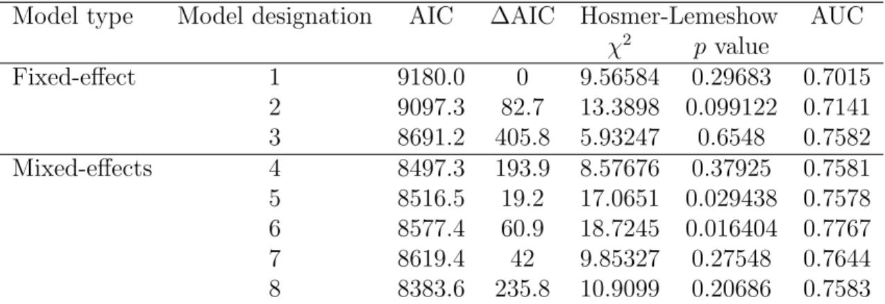
Table 3: The goodness-of-fit for the tested models.
Model type Model designation AIC ∆AIC Hosmer-Lemeshow AUC
χ2 p value Fixed-effect 1 9180.0 0 9.56584 0.29683 0.7015 2 9097.3 82.7 13.3898 0.099122 0.7141 3 8691.2 405.8 5.93247 0.6548 0.7582 Mixed-effects 4 8497.3 193.9 8.57676 0.37925 0.7581 5 8516.5 19.2 17.0651 0.029438 0.7578 6 8577.4 60.9 18.7245 0.016404 0.7767 7 8619.4 42 9.85327 0.27548 0.7644 8 8383.6 235.8 10.9099 0.20686 0.7583
1: Model considering stand variables, except slope classes. The hazard is constant over time. 2: Model 1 including slope classes.
3: Model 2 with a variation of hazard over time. 4: Model 3 with random effect of map element level 1 5: Model 3 with random effect of map element level 2 6: Model 3 with random effect of map element level 3 7: Model 3 with random effect of map element level 4 8: Model 3 with random effect of cruise line
∆AIC: Difference between the AIC value of the successive models.
The fit statistics revealed a substantial improvement in the maximum likelihood when random effects were included. The best fit was obtained with a cruise line random effect, which yielded an AIC of 8383.6 and an AUC of 0.7583. The final model had the following form:
Pr(yijk = 1) = 1 − e
−eβ1ln(BAijk)+β2Nijk+β3,s+β4,vPt2
z=t1eγ0+γ1AACz +ui (10)
where BAijk is the basal area (m2ha−1) of plot j in cluster i during interval k; N is the
stem density (stem ha−1); s is the index for the six different slope classes; v is the index for the three dynamics classes; AACz is the regional annual allowable cut volume (m3ha−1) for
year z; and ui is the cruise line random effect. For this model, the Hosmer-Lemeshow test
indicated no evidence of under- or overestimation and no violation of the model assumptions at p < 0.01. The predicted probabilities and the observed proportions for the 10 groups were plotted (Fig. 2).
Observed proportion 0.5 0.6 0.7 0.8 0.5 0.6 0.7 0.8 0.9 1.0 0.9 1.0 Predicted probability
Figure 2: Observed proportions and predicted probabilities of events evaluated by the Hosmer-Lemeshow test.
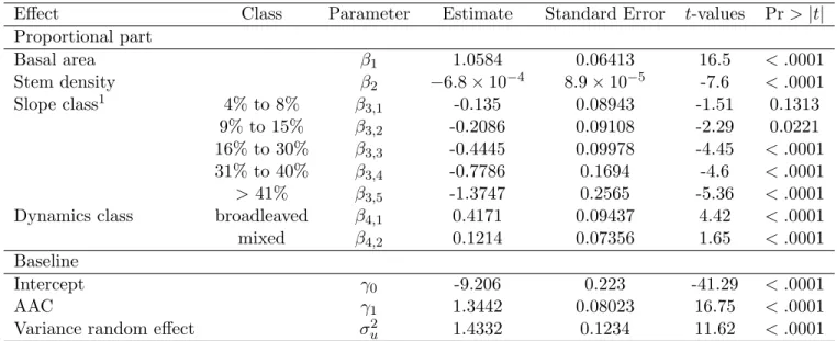
The resulting parameter estimates are shown in Table 4. The sign of the estimates indi-cates the influence on the predicted probabilities, with a positive sign indicating an increase in the probability of harvest and vice versa. In this respect, basal area increased the harvest probability. In contrast, stem density and slope classes decreased it. In addition, dynamics classes also showed a significant effect. Greater harvest probabilities were associated with the broadleaved dynamics class, followed by the mixed and the coniferous classes. Our results also indicated that reductions of the AAC induced a decrease in the harvest probabilities.
Table 4: Maximum likelihood estimates of the parameters in the final model (Model 8) with their associated standard errors and approximate t-values.
Effect Class Parameter Estimate Standard Error t-values Pr > |t| Proportional part Basal area β1 1.0584 0.06413 16.5 < .0001 Stem density β2 −6.8 × 10⁻⁴ 8.9 × 10⁻⁵ -7.6 < .0001 Slope class1 4% to 8% β3,1 -0.135 0.08943 -1.51 0.1313 9% to 15% β3,2 -0.2086 0.09108 -2.29 0.0221 16% to 30% β3,3 -0.4445 0.09978 -4.45 < .0001 31% to 40% β3,4 -0.7786 0.1694 -4.6 < .0001 > 41% β3,5 -1.3747 0.2565 -5.36 < .0001
Dynamics class broadleaved β4,1 0.4171 0.09437 4.42 < .0001
mixed β4,2 0.1214 0.07356 1.65 < .0001
Baseline
Intercept γ0 -9.206 0.223 -41.29 < .0001
AAC γ1 1.3442 0.08023 16.75 < .0001
Variance random effect σ2u 1.4332 0.1234 11.62 < .0001
1: Inclination
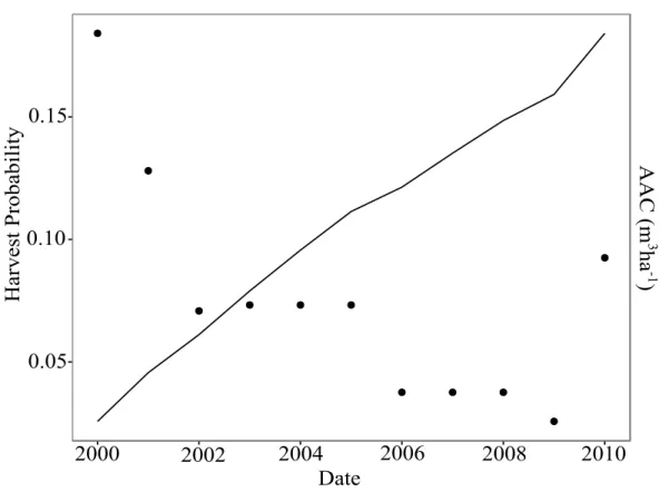
The Bas-Saint-Laurent administrative region was chosen to illustrate the predictions of the final model based on an average plot (Fig. 3). AAC values from 2000 to 2010, which ranged from 1.49 to 1.97 m3ha−1, were used for the baseline. For the lowest value of AAC, the
corresponding annual harvest probability was 0.013. For the highest AAC, this probability was 0.022. The effect of the AAC drop in 2006 could be detected in the cumulative probability since the increase for that year was smaller than those of previous years. The AAC increase in 2010 had exactly the opposite effect on the cumulative probability. Over the 10-year interval, that plot had a predicted probability of being harvested of close to 0.18.
0.10
0.05
0.15
Harvest Probability
Date
2000
2002
2004
2006
2008
2010
AAC (
m
3ha
-1)
Figure 3: Simulation of the AAC effects on harvest probability for Bas-Saint-Laurent. The dots represent the values of AAC. The line represents the cumulative harvest probability. The reference values are: BA = 18 m2ha−1; slope = 4% to 8%; stem density = 725 m2ha−1;
and dynamics class = mixed.
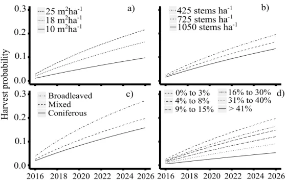
The effects of the other covariates on the predictions is shown in Fig. 4. Basal area had a considerable influence over the predicted harvest probabilities. The probability associated with the largest basal area was twice that of the lowest basal area, with values decreasing from 0.22 to 0.10 (Fig. 4a). An increase in stem density decreased the harvest probability, with a difference of about 0.06 between the highest and the lowest densities (Fig. 4b). The predicted probabilities for the broadleaved dynamics class were almost two times higher than those of the coniferous class, which exhibited the lowest probability with 0.16. For the mixed class, the estimated harvest probability was 0.20 (Fig. 4c). The steeper the slope, the lower the probabilities of harvest were (Fig. 4d).
Harvest probability 0.0 0.1 0.2 0.3 0.0 0.1 0.2 0.3 2016 2018 2020 2022 2024 2026 2016 2018 2020 2022 2024 2026 Broadleaved Mixed Coniferous c) a) b) d) 10 m2ha-1 18 m25 m2ha-1 2ha-1 1050 stems ha-1 425 stems ha-1 725 stems ha-1 Date > 41% 31% to 40% 4% to 8% 16% to 30% 9% to 15% 0% to 3%
Figure 4: Effect of the model variables on the predicted harvest probabilities for a 10-year interval. (a) basal area effect; (b) stem density effect; (c) dynamics class effect; (d) slope class effect. The reference values are: BA = 18 m2ha−1; slope = 4% to 8%; stem density =
725 m2ha−1; and dynamics class = mixed.
The different random effect specifications based on the map elements showed similar variance estimates. A small difference was found for the highest resolution, which had a variance estimate of 0.53. The variance of the cruise line random effect was larger by far than those of the map elements, with an estimated value of 1.43. For all tested models, neither the countervailing duty nor the exchange rates had significant contributions and, consequently, they were discarded from the model.
4
Discussion
In this study we used plot- and regional-level variables combined with spatial random effects to predict the plot-level harvest probability using a survival analysis approach. Our results showed the potential of survival analysis to provide annual predictions of harvest occurrence using a hazard function. Additionally, this approach allowed us to overcome limitations re-ported in the harvest literature, such as taking changes in economic conditions or legislation into account (Ant´on-Fern´andez and Astrup, 2012), as well as changes in management
prac-tices and length of intervals (Thurnher et al., 2011). Through this hazard function, a survival analysis can deal with uneven intervals and time-varying regional variables. It is definitely an easier and cheaper alternative than investing in additional field measurements. Thus, our modeling approach and the nature of the variables make this study an original contribution. Previous works on harvest predictions were primarily focused on harvest algorithms (e.g., Nelson and Finn, 1990; Liu et al., 2006; Heaps, 2015). More recently, the logistic regression was introduced as an effective method for modeling this kind of variable. These studies considered tree- and plot-level variables (e.g., Thurnher et al., 2011; Ant´on-Fern´andez and Astrup, 2012) but economic or political covariates acting at the regional level had been ignored so far. Moreover, the logistic regression shows some shortcomings when dealing with interval-censored data. It suffers from sample bias (Wang et al., 2013) if the sampling intensity changes over time. Also, it does not account for within-interval time-varying covari-ates. The market and the management strategy may change during the intervals and these changes cannot be taken into account in the logistic regression. Our results showed that the survival analysis approach provides enough flexibility to allow for these regional variables and can generate unbiased predictions of harvest occurrence, confirming our first and second hypotheses.
The hazard function used to generate plot harvest probabilities has two components: the baseline and the proportional part (Lawless, 2003, p. 36). We assumed that the covariates affecting the baseline were at the regional level and were allowed to vary within the intervals on an annual basis, whereas the plot-level variables belonged to the exponential part of the hazard function. In order to test our second and third hypotheses, we modeled the baseline as a function of the AAC, which allows the hazard to change over time within a given interval. This is the time-dependent part of the hazard. In contrast, the plot-level variables were considered as having a constant impact on the hazard over the interval.
In strategic planning that includes the assessment of sustainability, forestry actions have long-lasting effects and cover larger areas when compared to tactical planning (Kangas et al., 2001). In order to accomplish the strategic level decisions, our harvest model should be coupled with a growth model, which would allow the manager to account for business-as-usual scenarios and management variations. We therefore recommend our model as capable of predicting the harvesting probability on a long-term planning horizon. The general principles underlying our methods may be applicable to a wide range of forest types.
Model evaluation based on cross-validation has been criticized by some authors [e.g.,][](Kozak and Kozak, 2003). It turns out that the cross-validation does not provide much more informa-tion that what could be obtained with the whole dataset. We do agree with this statement. However, there is another benefit of using cross-validation, which is the detection of overfitted models. From our experience, it often happens that complex mixed-effects models converge with the whole dataset but not during the cross-validation. This is essentially due to a par-ticular fixed effect that is strongly related to a few plots. This happened with a preliminary version of the model. When this fixed effect was eliminated, the model then converged for all the runs of the cross-validation. This process ensured that the final model we obtained was the most parsimonious.
With respect to the tested covariates, we managed to quantify the importance and inten-sities of their effects. As expected, an increase in basal area induced an increase in harvest probability. In Quebec, dense stands are often submitted to different intensities of harvest
to meet various objectives, e.g., to increase timber yield, to promote natural succession, to regulate competition levels and to improve stand vigor (Majcen et al., 2003). Our plot-level harvest model reflected these management practices. Additionally, the results are also in accordance with Sterba et al. (2000) who found a similar relationship between the harvest probability and the natural logarithm of basal area in a clearcut regime in Austria.
The harvest probabilities decreased with increasing stem densities. This result can be explained by the fact that lower stem densities are found in mature stands (Bose et al., 2013). The influence of maturity on harvest probability was also reported in the study of Ant´on-Fern´andez and Astrup (2012). Moreover, for a given basal area, more stems means trees with lower individual volumes, which is less interesting from a commercial point of view. Lower harvest probabilities were found in the plots with steeper slopes, showing the obvious limitations related to harvest operations. In Quebec, harvesting on slopes of more than 40% is unusual and is authorized only for preventive measures (MNR, 1998).
The model predictions also confirmed that the dynamics class was a determining factor in the harvest occurrence. The broadleaved class showed greater probabilities of harvest. This pattern seems to be consistent with the management strategy in Quebec. Broadleaved species are more abundant in Southern Quebec, whereas coniferous species are dominant in the northern part of the commercial forest. There are obvious differences in the harvest intensity depending on the dynamics class. Until the 1990s, clearcutting and diameter-limit cutting were common practices but were found to be unsuitable for many vegetation types, which led to an evolution of management practices (Archambault et al., 1998). Since the 1990s, the most common treatment in the stands of the broadleaved dynamics class is selection cutting based on a cycle of 20 to 25 years (MFFP, 2013). For coniferous stands, the final cut at the end of the rotation, which lasts 50 years at best, is usually carried out, implying a harvesting of 90 to 99% of the merchantable volume (MFFP, 2013).
As regards regional-level variables, we also tested the exchange rate and countervailing duty as regional variables in the model. However, neither of them proved to have a significant effect on the harvest occurrence. This could be due to confounding effects with the AAC. As a matter of fact, the AAC drop in the mid 2000s coincides with a drop in the exchange rate and the implementation of the countervailing duty.
Spatial correlation has been extensively studied as well as its effects. One of the benefits of considering spatial correlation is the better consistency in parameter estimates (Bhat and Sener, 2009). It also plays an important role in harvest scheduling since different spatial patterns influence some economic and conservation objectives (BoWang and Gadow, 2006).
In our model, we used random effects to account for these spatial correlations. The cluster random effect resulted in an improvement of the model fit. This random effect can be interpreted as a trend for plots belonging to the same cruise line to jointly deviate from the expected value. This is not surprising if we compare the area covered by a cruise line with the area of cut blocks. The correlations between the map elements at different resolutions were smaller but non-negligible. These correlations over larger areas could be explained by management practices. Until recently, forest companies planned their annual operation by sectors, which means that the stands of these sectors were more likely to be harvested at the same time as those of other sectors. If the harvest model was to be used for tactical planning, it could eventually be improved by integrating the geographical information of the tactical plans, which is not really possible in strategic planning over large areas.
Multiple random effects with the cruise lines nested in the map elements were also tested. In spite of our efforts to fit this model, convergence problems were a limiting aspect. An alternative approach to random effects would be the direct modeling of spatial correlations. The inclusion of a copula could be an example. Thus, further improvements in terms of the described limitations still remain as possible points of investigation.
In conclusion, this study proposed an alternative approach to model plot-level harvest occurrence. Our approach combined survival analysis with time-varying variables, taking uneven intervals and censored observation data into account.
Regarding our hypotheses, we can conclude that the survival analysis approach can be used to obtain unbiased predictions of plot-level harvest occurrence. Secondly, the inclusion of variables at the regional level, such as AAC, had a significant effect on harvest probabilities. The inclusion of such a time-varying explanatory variable in the model significantly increased its likelihood, which was the third hypothesis. In the context of forest management, such a multi-level approach could be useful in strategic planning. Coupled to a growth model, it makes it possible to generate large-area growth predictions for forests under management.
Acknowledgements
The authors wish to thank the Direction des inventaires forestiers of the Minist`ere des Forˆets, de la Faune et des Parcs du Qu´ebec for the permanent-plot data. This work is part of the first author’s PhD thesis, supported by the National Counsel of Technological and Scientific Development of Brazil - CNPq. The UMR 1092 LERFoB is supported by a grant overseen by the French National Research Agency (ANR) as part of the “Investissements d’Avenir” program (ANR-11-LABX-0002-01, Lab of Excellence ARBRE).
References
Allison, P. D. (1982). Discrete-time methods for the analysis of event histories. Sociological Methodology, 13:61–98.
Ant´on-Fern´andez, C. and Astrup, R. (2012). Empirical harvest models and their use in regional business-as-usual scenarios of timber supply and carbon stock development. Scandinavian Journal of Forest Research, 27:379–392.
Archambault, L., Morissette, J., and Bernier-Cardou, M. (1998). Forest succession over a 20-year period following clearcutting in balsam fir-yellow birch ecosystems of eastern quebec, canada. Forest Ecology and Management, 102:61–74.
Bhat, C. and Sener, I. (2009). A copula-based closed-form binary logit choice model for accomodating spatial correlation across observational units. J. Geogr Syst, 11:243–272. Bose, A., Harvey, B., Brais, S., Beaudet, M., and Leduc, A. (2013). Constraint to partial
cut-ting in the boreal forest of canada in the context of natural disturbance-based management: a review. Forestry, 87:11–28.
Boulay, E. (2013). Ressources et industries Foresti`eres - Portrait statistique - Edition 2013. Technical report, Minist`ere des Ressources naturelles, Gouvernement du Qu´ebec, Canada. Boulay, E. (2015). Ressources et industries Foresti`eres - Portrait statistique - Edition 2015. Technical report, Minist`ere des Forˆets, de la Faune et des Parcs, Gouvernement du Qu´ebec, Canada.
BoWang, C. and Gadow, K. (2006). Timber harvest planning with spatial objectives, using the method of simulated annealing. European Journal of Forest Research, 121:25–34. Descˆoteaux, D. and Martin, P. (2009). D´esunis dans l’adversit´e: Les consommateurs
am´ericains et le conflit du bois duvre entre le canada et les ´etats-unis. Revue ´Etudes internationales, 40:373–394.
Dong, L., Bettinger, P., Z Liu, Z., and Qin, H. (2015). A comparison of a neighborhood search technique for forest spatial harvest scheduling problems: A case study of the simulated annealing algorithm. Forest Ecology and Management, 356:124–135.
Firth, D. (1993). Bias reduction of maximum likelihood estimates. Biometrika, 80:27–38. Fortin, M. (2013). Population-averaged predictions with generalized linear mixed-effects
models in forestry: an estimator based on gauss-hermite quadrature. Canadien Journal of Forest Research, 43:129–138.
Fortin, M. (2014). Using a segmented logistic model to predict trees to be harvested in forest growth forecasts. Forest Systems, 23:139–152.
Fortin, M., Delisle-Boulianne, S., and Pothier, D. (2013). Considering spatial correlations between binary response variables in forestry: an example applied to tree harvest modeling. Forest Science, 59:253–260.
Heaps, T. (2015). Convergence of optimal harvesting policies to a normal forest. Journal of Economic Dynamics and Control, 54:74–85.
Hernandez, M., G´omez, T., Molina, J., Le´on, M., and Caballero, R. (2014). Efficiency in forest management: A multiobjective harvest scheduling model. Journal of Forest Economic, 20:236–251.
Kangas, J., Kangas, A., Leskinen, P., and Pykalainen, J. (2001). Mcdm methods in strategic planning of forestry on state-owned lands in finland: Applications and experience. Journal of Multi-Criteria Decision Analysis, 10:257–271.
Kozak, A. and Kozak, R. (2003). Does cross validation provide additional information in the evaluation of regression models? Canadien Journal of Forest Research, 33:976–987. Lawless, J. (2003). Statistical Models and Methods for Lifetime Data. John Wiley and Sons,
Hoboken.
Liu, G., Han, S., Zhao, X., Nelson, J., Wang, H., and Wang, W. (2006). Optimisation algorithms for spatially constrained forest planning. Ecological Modelling, 194:421–428. Majcen, Z., B´edard, S., and Godbout, C. (2003). La forˆet feuillue du Qu´ebec et la recherche
en sylviculture. Technical report, Note de recherche foresti´ere - Gouvernement du Qu´ebec, Canada.
Manso, R., Morneau, F., Ningre, F., and Fortin, M. (2015). Incorporating stochasticity from extreme climatic events and multi-species competition relationships into single-tree mortality models. Forest Ecology and Management, 354:243–253.
Martell, D., Gunn, E., and Weintraub, A. (1998). Forest management challenges for opera-tional researchers. European Journal of Operaopera-tional Research, 104:1–17.
McCullagh, P. (2008). Sampling bias and logistic models. Journal of Royal Statistic Society, 70:643–677.
McCulloch, C., Searle, S., and Neuhaus, J. M. (2008). Generalized, linear, and mixed models. John Wiley & Sons, New York.
MFFP (2003). Manuel d’am´enagement forestier. Technical report, Minist`ere des Forˆets, de la Faune et des Parcs, Gouvernement du Qu´ebec, Canada.
MFFP (2013). Manuel de d´etermination des possibilit´es foresti´eres 2013-2018. Technical report, Bureau du forestier en chef, Gouvernement du Qu´ebec, Canada.
MFFP (2014). R´eseaux des placettes-´echantillons permanentes du Qu´ebec m´eridional. Tech-nical report, Direction des inventaires forestiers, Minist`ere des Forˆets, de la Faune et des Parcs, Gouvernement du Qu´ebec, Canada.
Miina, J. (1996). Optimizing thinning and rotation in a stand of pinus sylvestris on a drained peatland site. Scandinavian Journal of Forest Research, 11:182–192.
MNR (1998). Guide des saine pratiques foresti´eres dans les pentes du Qu´ebec. Technical report, Minist´ere des Ressources naturelles, Gouvernement du Qu´ebec, Canada.
Nelson, J. and Finn, S. (1990). The influency of cut-block size and adjacency rules on harvest levels and road networks. Canadien Journal of Forest Research, 21:595–600.
Parent, B. (1988). Ressources et industries Foresti`eres. Technical report, Minist`ere des Ressources naturelles, Gouvernement du Qu´ebec, Canada.
Parent, B. (1990). Ressources et industries Foresti`eres. Technical report, Minist`ere des Ressources naturelles, Gouvernement du Qu´ebec, Canada.
Parent, B. (1992). Ressources et industries Foresti`eres. Technical report, Minist`ere des Ressources naturelles, Gouvernement du Qu´ebec, Canada.
Parent, B. (1993). Ressources et industries Foresti`eres. Technical report, Minist`ere des Ressources naturelles, Gouvernement du Qu´ebec, Canada.
Parent, B. (1994). Ressources et industries Foresti`eres. Technical report, Minist`ere des Ressources naturelles, Gouvernement du Qu´ebec, Canada.
Parent, B. (1996). Ressources et industries Foresti`eres. Technical report, Minist`ere des Ressources naturelles, Gouvernement du Qu´ebec, Canada.
Parent, B. (1999). Ressources et industries Foresti`eres - Portrait statistique - Edition 1999. Technical report, Minist`ere des Ressources naturelles, Gouvernement du Qu´ebec, Canada. Parent, B. (2009). Ressources et industries Foresti`eres - Portrait statistique - Edition 2009. Technical report, Minist`ere des Ressources naturelles, de la Faune, Gouvernement du Qu´ebec, Canada.
Parent, B. (2010). Ressources et industries Foresti`eres - Portrait statistique - Edition 2010. Technical report, Minist`ere des Ressources naturelles, de la Faune, Gouvernement du Qu´ebec, Canada.
Parent, B. and Fortin, C. (2000). Ressources et industries Foresti`eres - Portrait statistique - Edition 2000. Technical report, Minist`ere des Ressources naturelles, Gouvernement du Qu´ebec, Canada.
Parent, B. and Fortin, C. (2002). Ressources et industries Foresti`eres - Portrait statistique - Edition 2002. Technical report, Minist`ere des Ressources naturelles, Gouvernement du Qu´ebec, Canada.
Parent, B. and Fortin, C. (2003). Ressources et industries Foresti`eres - Portrait statistique - Edition 2003. Technical report, Minist`ere des Ressources naturelles, de la Faune et des Parcs, Gouvernement du Qu´ebec, Canada.
Parent, B. and Fortin, C. (2004). Ressources et industries Foresti`eres. Technical report, Minist`ere des Ressources naturelles, Gouvernement du Qu´ebec, Canada.
Parent, B. and Fortin, C. (2005). Ressources et industries Foresti`eres - Portrait statistique - Edition 2004. Technical report, Minist`ere des Ressources naturelles, de la Faune, Gou-vernement du Qu´ebec, Canada.
Parent, B. and Fortin, C. (2006). Ressources et industries Foresti`eres - Portrait statistique - Edition 2005-2006. Technical report, Minist`ere des Ressources naturelles, de la Faune, Gouvernement du Qu´ebec, Canada.
Parent, B. and Fortin, C. (2007). Ressources et industries Foresti`eres - Portrait statistique - Edition 2007. Technical report, Minist`ere des Ressources naturelles, de la Faune, Gou-vernement du Qu´ebec, Canada.
Parent, B. and Fortin, C. (2008). Ressources et industries Foresti`eres - Portrait statistique - Edition 2008. Technical report, Minist`ere des Ressources naturelles, de la Faune, Gou-vernement du Qu´ebec, Canada.
Parent, G., Boulay, E., and Fortin, C. (2012). Ressources et industries Foresti`eres - Portrait statistique - Edition 2012. Technical report, Minist`ere des Ressources naturelles, de la Faune, Gouvernement du Qu´ebec, Canada.
Pinheiro, J. and Bates, D. (1995). Approximations to the log-likelihood function in the nonlinear mixed-effects model. Journal of Computational and Graphical Statistics, 4:12– 35.
Pinheiro, J. and Bates, D. (2000). Mixed effects models in S and S-PLUS. Springer, New York.
Pukkala, T. and Kurttila, M. (2005). Examining the performance of six heuristic optimisation techniques in different forest planning problems. Silva Fennica, 39:67–80.
Pukkala, T., Miina, J., Kurttila, M., and Kolstrom, T. (1998). A spatial yield model for opti-mizing the thinning regime of mixed stands of pinus sylvestris and picea abies. Scandinavian Journal of Forest Research, 13:31–42.
Rahman, O. and Devadoss, S. (2002). Economics of the uscanada softwood lumber dispute: A historical perspective. Journal of International Law and Trade Policy, 52:29–45.
Rose, C. E., Hall, D. B., Shiver, D. B., Clutter, M. L., and Border, B. (2006). A multilevel approach to individual tree survival prediction. Forest Science, 52:31–43.
Sample, V. A. (2004). Sustainability in forestry: Origins, evolution and prospects. Technical report, Pinchot Institute for Conservation.
SAS (2015). SAS/STAT 14.1 User’s Guide. SAS Institute Inc., Cary, North Carolina, USA. Saucier, J.-P., Robitaille, A., and Grondin, P. (2009). Cadre bioclimatique du Qu´ebec.
´
Editions Multimondes, Qu´ebec, Canada.
Sterba, H., Golser, M., Moser, M., and Schadauer, K. (2000). A timber harvesting model for austria. Computers and Electronics in Agriculture, 28:133–149.
Thurnher, C., Klopf, M., and Hasenauer, H. (2011). Forests in transition: a harvesting model for uneven-aged mixed species forests in austria. Forestry, 84:517–526.
Wang, N., Brown, D., Yang, S., and Ligmann-Zielinska, A. (2013). Comparative performance of logistic regression and survival analysisfor detecting spatial predictors of land-use change. International Journal of Geographical Information Science, 27:1960–1982.
Willet, J. and Singer, J. (1993). Investigating onset, cessation, relapse, and recovery: Why you should and how you can use discrete-time survival analysis to examine event ocurrence. Journal of consulting and clinical psychology, 61:952–965.
A
Implementation of the model using the NLMIXED
procedure
The annual AACs are contained in the 1988-2014 period, therefore, a total time interval of 27 years.
************************************************************** * Implementation in SAS: Survival Analysis using Proc NLMIXED **************************************************************
data= data set RE = random effect
parameterestimates = output parameters T-V = time-varying variable
out = output dataset
beta = vector of parameters
x = vector of explanatory variables EO = event ocurrence
proc sort data=; by RE; run;
ods output parameterestimates = myEstimates; proc nlmixed data= technique=NRRIDG gconv=;
where year >= 1988; title "Model 8";
parms beta1 = 1 beta2 = 1 beta3 = 1 beta4 = 1 gamma0 = 1 gamma1 = 1;
array AAC[27] AAC 1988-AAC2014;
array dummy[27] d1988-d2014; SAnnee = 0;
do Year = 1 to 27;
hazard = SAnnee + exp(gamma0 + gamma1 AAC [27] + u) dummy[27];
end;
proportional = beta x ;
SCond = exp(-exp(proportional)hazard); S = SCond**exp(u);
Likelihood = EO * log(S) + (1 - EO) * log(1-S);
model EO ~ general(Likelihood);
random u ~ normal(0, s2u) subject= RE; predict SCond out= ;
run