Relation between entropy, free energy and computational energy

To cite this version :

Maxence BIGERELLE, Hisham ABDEL-AAL, Alain IOST - Relation between entropy, free energy and computational energy Int. J. Materials and Product Technology Vol. 38, n°1, p.3543 -2010

Relation between entropy, free energy

and computational energy

Maxence Bigerelle*

Centre de Recherches de Royallieu BP20529, 60205 Compiègne, France

E-mail: maxence.bigerelle@utc.fr *Corresponding author

Hisham A. Abdel-Aal

Laboratoire de Mécanique et Procédé de Fabrication (LMPF, EA4106), Arts et Metier ParisTech, LMPF,

Rue Saint Dominique BP 508, 51006, Chalons-en-Champagne, France

E-mail: hisham.abdel-aal@chalons.ensam.fr

Alain Iost

Arts et Metiers ParisTech, CNRS, LMPGM, 8, Boulevard Louis XIV, 59046 Lille Cedex, France Fax: 33(0)3 20 62 29 57

E-mail: alain.iost@ensam.eu E-mail: alain.iost@lille.ensam.fr Abstract: This paper proposes an isomorphism between the number of accessible states of the system including statistical fluctuation and the optimised size of a computer program set-up by combining the Huffman and R.L.E algebrae. At first, a relation between the variation of the free energy in the system and the variation of the programme size used to describe the system was stated. A fluctuation to the equilibrium decreases the size of the programme in relation to the decrease in entropy and the decay of the free energy of the system.

Keywords: entropy; energy; information theory; data compression; Monte Carlo simulation.

Reference to this paper should be made as follows: Bigerelle, M., Abdel-Aal, H.A. and Iost, A. (2010) ‘Relation between entropy, free energy and computational energy’, Int. J. Materials and Product Technology, Vol. 38, No. 1, pp.35–43.

Biographical notes: Maxence Bigerelle is a Professor in Materials Science, Engineer in Computer Sciences, PhD in Mechanics and Material Sciences (1999), Medical Expert in Biomaterials at the University Hospital Centre of Lille, Capacitation of Research. Directorship in Physical Sciences (2002). Field of interests: surfaces and interfaces morphological characterisation,

36 M. Bigerelle et al.

multi-scale modelling, fractal and chaos, biomaterials and nanostructures. Director Assistant of the Materials Research Group in the Laboratory Roberval, UMR 6253, UTC/CNRS, Centre de Recherches de Royallieu, BP20529, 60205 Compiegne France.

Hisham A. Abdel-Aal obtained his Doctoral Degree from the University of North Carolina in Charlotte in Mechanical Engineering. He taught at the University of Wisconsin and is currently an Invited Research Professor at Arts et Métier ParisTech. He is interested in problems of tribology at all scales and in the thermodynamic behaviour and stability of tribological systems.

Alain Iost is a Professor of Metallurgy and Materials Science at ‘ENSAM Lille’ and leader of the team “Characterisation and Properties of Perisurfaces” at the Physical Metallurgy and Material Engineering Laboratory. The main fields of interests are the mechanical and morphological characterisation of the surfaces and interfaces.

1 Introduction

The equal a priori probability postulate is fundamental to all statistical mechanisms and allows full discussion of the properties of systems at equilibrium. By supposing time-differentiable systems when probabilities and transition probabilities are well known, i.e., for an infinite, and isolated system, theorems like the H one give only mathematical conditions. However, numerous systems cannot be considered as infinite and then have some intrinsic fluctuations. Under these conditions, the term ‘equilibrium’ has to be defined more precisely. In thermodynamic formalism, the final time-independent equilibrium situation is reached if the distribution of the system over these accessible states remains uniform (i.e., randomly uniform). The definition of equilibrium is then reduced to the definition of randomness. Since Chaitin (1987) shows, using the theory of information (Shannon, 1948; Brillouin, 1956), that randomness depends on algorithmic complexity, we have chosen to analyse the system in terms of data compression rather than quantify information by purely theoretical mathematical objects. The higher the information, the lower the ratio of data compression. By unifying these different theories and to shortly summarise our theoretical approach, we postulate as an axiom that a system will be integrally described if the size of the system after compression by applying all data compression algorithms is minimal. Since the data compression algorithms entail the knowledge of the physical system, the size of the programme becomes a mathematical measure of Negentropy. Negentropy, corresponding to negative entropy, that represents the quality or grade of energy must always decrease and is at the foundation of Kelvin’s principle of ‘degradation of energy’. Under some adequate properties of the data compression algorithm, we proved in a recent paper (Bigerelle and Iost, 2002) that it is possible to quantify the rate of the diffusion states, which implies that the average information contained by the diffusion process can be described by this theory. The aim of this paper is to analyse whether the same approach can allow us to quantify fluctuations around equilibrium and to compare these relations to those obtained by statistical thermodynamics. Finally, we shall show that a linear relation exists between the computational energy and the physical energy of the system.

2 Mathematical definitions

The mathematical definitions that will be used to deal with our thermodynamic system are first briefly introduced (all formalisms with proofs will be published later).

Let X be a set (discretised system), T the bijective algebra that transforms the system X into a system Y, noted Y = T(X), and Card(X) is the size of the X set.

T(X) is said contractile if

card( ( )) card( ).T X ≤ X (1)

Example: 100 particles follow the Fermi-Dirac statistics law with 100 possible states.

The set X is defined by X = {1, 1, …, 1} and then card(X) = 100 (the elementary unit is the bit). Let us define the T algebra by writing X states in a decimal notation. Then, card(T(X)) = R[log2(card(X))], where R[z] rounded z to the higher integer.

As card(T(X)) = R[log2(100)] = 7, then card(T(X)) ≤ card(X) meaning that T(X) is

contractile.

Let {A} be a set of algebra, F is said {A}-maxi contractile in Ω if there exists one algebra noted Tmin∈ {A} such that:

min

, { }, card( ( , )) card( ( , )).

X T A F X T F X T

∀ ∈ Ω ∀ ∈ ≤ (2)

F(X) is said {∞}-maxi contractile in Ω, F is maxi contractile in Ω for all the sets of all possible algebrae defined by arithmetics.

Theorem 1: There exists at least one maxi-contractile algebra in _Ω.

Theorem 2: The arithmetic method is unable to construct the algebra Tmin∈ {∞}.

Theorem 3: It is always possible to find an algebra T ∈ {∞} for any subset x

such that: α(T)card(F(x, Tmin)) ≤ card(F(x, T)) ≤ β(T)card(F(x, Tmin)), α(T) ≥ 1, β(T) ≥ 1,

α(T) < β(T).

3 Fluctuation of a system at equilibrium 3.1 Thermodynamic description

An isolated system A represented by a B2 _{Boolean matrix noticed A(B) (0: empty; 1: full)}

with 50% of full cells (maximal entropy). At equilibrium, the probability P of finding A follows P ∝ Ω where Ω is the number of accessible states. As a result from the statistical fluctuations, the system deviates from its equilibrium state. The classical thermodynamic approach consists in dividing A into two equal parts with N + k exciting states in the first part and N − k in the second and therefore:

( ) 2 !/(( )!( )!).

k N N N k N k

Ω = + − (3)

The maximal value, Ω0(N), is the configuration of the average equilibrium state. Using

the classical Stirling approximation, the well-known relation is obtained: 2

0exp( / )

k n N

38 M. Bigerelle et al.

which is a Gaussian Probability Density Function (PDF) if an adequate normalisation is performed.

3.2 Algebra description

At this stage, the terms Ω0 must be analysed by the information theory.

Theorem 4: There exists F{∞}-maxi ultimately uniformly contractile in A(B), F is

independent of B (B finite) such that F is said Ω(A(B), Tmin, k) -pertinent:

min min

dΩ_k/ dk=_α(T )d ( ( ),F A B T , ) / d .k k (5)

This theorem clearly entails that a linear relation exists between the Ω fluctuations (entropy fluctuation) and the size of an adequate algorithm based on a Tmin algebra.

As Tmin cannot be constructed (Theorem 2), only an approximation can be given

(Theorem 4). We have shown (Bigerelle and Iost, 2002) that a good approximation that reduces _{β(T) −α(T) is obtained by composing both R.L.E (Salomon, 1998) and Huffman} algebra (Huffman, 1952) noted ( ( , RLE), Huf )F F X =F X( , Huf RLE)D .

3.3 Numerical simulation of equilibrium

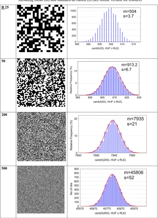
Two integer random numbers a and b (a ≤ B, b ≤ B) representing the position (a, b) of a cell A(B) and a Boolean random number c representing its state are chosen to construct the set A(B) at equilibrium. This same step is reproduced until the number of active cells reaches B2_{/2 (Fermi-Dirac statistics). 1000 systems A(B) are simulated}

with different sizes (B ∈ {25, 75, 100, …, 1000}) and their associated values card(F(A(B), Huf È RLE)) are calculated. Figure 1 represents snapshots of different system sizes with the empirical PDF (E − PDF(B)) of card( ( ( ), Huf RLE))F A B D in computer byte units. On these densities, we have calculated the mean and the standard deviation and plotted the Gaussian curves. Two remarks can be inferred:

• They follow Gaussian density. However, a discretisation effect appears for small system sizes.

• Both the mean and the standard deviation increase with the system size B.

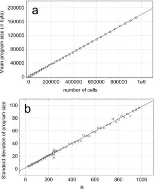
For the 1000 simulations performed for different system sizes B, the mean values of the programme size noticed card( ( ( ), Huf RLE))F A B D and the standard deviation are calculated. Figure 2(a) is a linear representation of the mean values vs. the number of elementary cells n = B2_:

2

0.00004 6

card( ( ( ), Huf RLE))F A B D =0.18040B± +605± (6)

where the intercepted value (605) representing the implementation size of the algebra can be seen as the handle of the programme compression.

From Figure 2(b), the standard deviation follows the regression equation: std

0.004 0.1

Figure 1 Four random systems with sizes B ∈ {25, 50, 200, 500} for A(B) systems at equilibrium and their associated empirical probability density functions of card(F(A(B), Huf È RLE) including mean (m) and standard deviation (s) (see online version for colours)

40 M. Bigerelle et al.

Figure 2 Mean (a) and standard deviation (b) of program size (in byte) obtained from 1000 simulations performed for different system sizes B ∈ {25, 75, 100, …, 1000}

3.4 Interpretation of the simulation

By introducing Ω =₀ 1/ _πN for the purpose of normalisation in probability

(

∑

)

In equation (3), the system contains 2N cells and then N = B2_{/4. Neglecting the intercept}

(B large enough) in equation (6), an elementary cell contains in mean 0.18 byte at equilibrium and then an active one represents 0.18 × 2 = 0.36 byte. As a consequence, a linear relation exists between k fluctuations and the size of a programme related to the computer cost:

One computer unit: I = 0.36. (8)

After normalisation, equation (4) follows a Gaussian zero-centred with the following standard deviation:

/ 2 ² / 4 / 2 / 2 2.

k N B B

σ = = = (9)

By neglecting the intercept in equation (7), equation (9) leads to: std

card( ( ( ), Huf RLE))F A B D =2 2 0.00966σk =0.27 .σk (10)

Therefore, the correspondence between the size of the programme and the states of the distribution will exist if: std

card( ( ( ), Huf RLE))F A B D =Iσk. The value 0.27 in

independent of the system size B, is an intrinsic measure of an isomorphism between the programme size and the number of accessible states of the system.

As the Gaussian PDF is defined by its mean and its standard deviation, the relation between the computer size and the number of states of the system is given by:

(

)

2

card( ( ( ), Huf RLE))

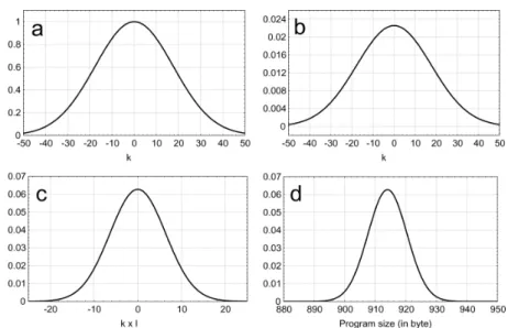
1/ ² / 4 exp . ( ² / 4)( ) k kI F A B I B B I π  −  ′′′ Ω = −     D (11) Considering B = 50, we shall now summarise with an example that all the

transformations allow us to transform the number of states of the system into a programme size (Figure 3).

Figure 3 Different isomorphic transformations for the state function of an equilibrium system of B = 50 into the size of the program in byte used to described the

thermodynamical system

Step 1: Calculation of the state functions Ωk(502/4). For k varying from −200 to 200,

2 2 (2(50² / 4))!_{exp( /(50² / 4)).} ((50² / 4)!) k k Ω = −

Step 2: Normalisation in probability. Multiplying the abscissa by 1/ π50² / 4 gives the following PDF: _{1/ 50² / 4 exp(} 2_{/(50² / 4)).}

k π k

′

Ω = −

Step 3: Scaling Ωk′ into information units:

2 0.18k 1/ 0.36 50² / 4 exp _{(50² / 4)(0.36)}2 . k π   ′′ Ω = −   

Step 4: Translation of Ω0.18k′′ to the mean value card( ( (50), Huf RLE))F A D =913. The final PDF is:

42 M. Bigerelle et al. 2 2 (0.36 913) 1/ 0.36 50² / 4 exp . (50² / 4)(0.36) k k π  −  ′′′ Ω = −   

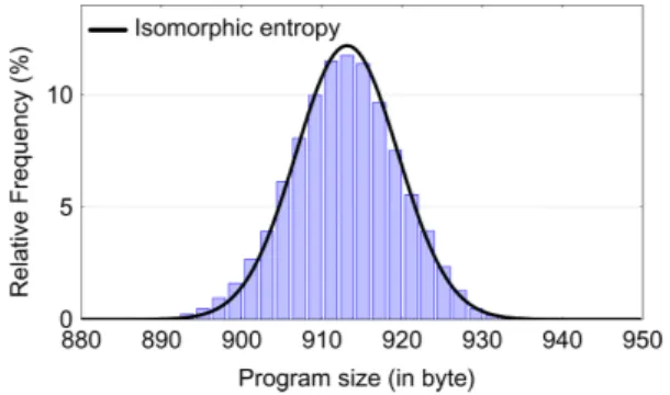
Figure 4 represents the variation of the programme size (box) and the theoretical density probability (solid line) defined by the isomorphism between the number of accessible states of the system (including statistical fluctuations) and the size of an optimised computer programme constructed with the composition of two algebra Huf RLED . The good agreement seems to conclude that the algebra Huf RLED tends to be maxi-ultimately-uniformly-contractile to allow us to describe the thermodynamic equilibrium system and its fluctuations.

Figure 4 Comparison of the program size (in byte) defined by the isomorphism on the entropy given by equation (11) (solid line) with the experimental values (box) obtained by the Monte Carlo simulation for a system size of B = 50 (see online version for colours)

4 Relation between entropy and free energy with computational energy

The fluctuations of the number of accessible states Ωn around the maximum value Ω0

(the most probable state) depend on an entropy fluctuation ∆Sn by the Bolzmann

formulae equation (4) and leads to: ln( ) n n S k ∆ = ∆ Ω (12) where 2 0 ln( _n) ln( _n) ln( ) n . N ∆ Ω = Ω − Ω = − (13)

Equations (12) and (13) show that entropy will always be decreased when the system fluctuates around the most probable state. From equation (8), we get

2 1 0 1 , I n n I πN Ω  ′′ Ω =   Ω  

then from equation (13) 0

ln n Sn

K

Ω ₌∆

2 0 ln n . n S kI Ω′′ ∆ =  _′′ Ω   (14)

Since the internal energy is null, the free energy of the system resulting from fluctuations is: 2 0 0 ln n ln n 0. n G Tk Ω  TkI Ω′′ ∆ = − _Ω = − _Ω′′≥     (15)

Fluctuation from equilibrium decreases the programme size that decreases the entropy and increases the free energy of the system. Within I2 _{factor, the gain of information in}

bit of the programme seems to be transformed into energy in the system.

5 Conclusion

We have shown that there exists a duality between the variation of the free energy of an isolated system and the variation of the programme size used to describe it, if this programme satisfies a maxi-ultimately-uniformly-contractile algebra. A fluctuation towards equilibrium decreases the size of the programme that decreases the entropy and increases the free energy of the system. Under the above hypotheses, the computer energy used to simulate the systems can be considered as similar to the free energy of the system (to within a constant factor).

References

Bigerelle, M. and Iost, A. (2002) ‘A new method to calculate the fractal dimension of an interface application to a Monte Carlo diffusion process’, Computer Mat. Sci., Vol. 24, pp.133–138. Brillouin, L. (1956) Science and Information Theory, Academic Press, New York.

Chaitin, G.J. (1987) Algorithmic Information Theory, Cambridge University Press, London. Huffman, D. (1952) ‘A method for the construction of minimum-redundancy codes’, Proc. IRE,

Vol. 40, No. 9, pp.1098–1101.

Salomon, D. (1998) Data Compression, Springer, New York.

Shannon, C.E. (1948) ‘A mathematical theory of communication’, Bell System Technical Journal, Vol. 27, pp.379–423 and 623–656.