2013 — Theoretical and numerical methods uses as design tool for an aircraft : application on three real-world configurations

MANUSCRIPT-BASED THESIS PRESENTED TO ÉCOLE DE TECHNOLOGIE SUPÉRIEURE

IN PARTIAL FULLFILMENT OF THE REQUIREMENTS FOR THE DEGREE OF DOCTOR OF PHILOSPHY

Ph. D.

BY

Nicoleta ANTON

THEORETICAL AND NUMERICAL METHODS USED AS DESIGN TOOL FOR AN AIRCRAFT: APPLICATION ON THREE REAL-WORLD CONFIGURATIONS

MONTRÉAL, AUGUST 5 2013

© Copyright reserved

It is forbidden to reproduce, save or share the content of this document either in whole or in parts. The reader who wishes to print or save this document on any media must first get the permission of the author.

BOARD OF EXAMINERS

THIS THESIS HAS BEEN EVALUATED BY THE FOLLOWING BOARD OF EXAMINERS

Dr. Ruxandra Botez, Thesis Supervisor

Département de génie de la production automatisée à l’École de technologie supérieure

Mr. François Morency, President of the Board of Examiners

Département de génie mécanique à l’École de technologie supérieure

Mr. Louis Dufresne, Member of the Board of Examiners

Département de génie mécanique à l’École de technologie supérieure

Mr. Adrian Hiliuta, External Member of the Board of Examiners CMC ELECTRONICS - ESTERLINE

THIS THESIS WAS PRESENTED AND DEFENDED

IN THE PRESENCE OF A BOARD OF EXAMINERS AND PUBLIC ON JULY 16, 2013

ACKNOWLEDGMENT

The research presented in this thesis has been carried out at the Department of Automated Production Engineering, Laboratory of Applied Research in Active Controls, Avionics and AeroServoElasticity (LARCASE) at École de Technologie Supérieure.

First and foremost I want to thank my advisor, Dr. Ruxandra Botez for her continued encouragement and invaluable suggestions during this work. I am also thankful for the excellent example she has provided as a successful woman in the aerospace field and as a professor. I would like to acknowledge the financial and academic support that provided the required research support.

Special thanks go to CAE Inc. for the invaluable experimental data provided for Hawker 800XP aircraft and to the CRIAQ (Consortium for Research and Innovation in Aerospace in Quebec) for the funding of the CRIAQ 3.2 project. I want to thank Dr. Andreas Schütte from the German Aerospace Centre (DLR) and Dr. Russell Cummings from the USAF Academy for their leadership and support in NATO RTO (Research & Technology Organization) AVT–161 « Assessment of Stability and Control Prediction Methods for NATO Air and Sea Vehicles” and for providing the wind tunnel test data within the DNW-NWB for the X-31 aircraft.

Thanks are also due to Mr Dumitru Popescu for his dedication in this work as well as to the other students from LARCASE who worked together on this project: Arnaud Vergeon, Chandane Zagjivan and Frédéric Lidove.

Finally, I want to express a huge thank you to my family. The encouragement and support I received from my beloved husband Adrian and my daughter Sarah Jade was a powerful source of inspiration and energy. Without them I would be a very different person, and it would have certainly been much harder to finish a PhD. Still today, learning to love him and

to receive his love makes me a better person. Last but not least, a very big thank you to my sister Ramona Venera and to my parents for their never-ending support.

THEORETICAL AND NUMERICAL METHODS USED AS DESIGN TOOL FOR AN AIRCRAFT: APPLICATION ON THREE REAL-WORLD CONFIGURATIONS

Nicoleta ANTON ABSTRACT

The mathematical models needed to represent the various dynamics phenomena have been conceived in many disciplines related to aerospace engineering. Major aerospace companies have developed their own codes to estimate aerodynamic characteristics and aircraft stability in the conceptual phase, in parallel with universities that have developed various codes for educational and research purposes.

This paper presents a design tool that includes FDerivatives code, the new weight functions method and the continuity algorithm. FDerivatives code, developed at the LARCASE laboratory, is dedicated to the analytical and numerical calculations of the aerodynamic coefficients and their corresponding stability derivatives in the subsonic regime. It was developed as part of two research projects. The first project was initiated by CAE Inc. and the Consortium for Research and Innovation in Aerospace in Quebec (CRIAQ), and the second project was funded by NATO in the framework of the NATO RTO AVT–161 «

Assessment of Stability and Control Prediction Methods for NATO Air and Sea Vehicles” program. Presagis gave the « Best Simulation Award" to the LARCASE laboratory for FDerivatives and data FLSIM applications. The new method, called the weight functions method, was used as an extension of the former project. Stability analysis of three different aircraft configurations was performed with the weight functions method and validated for longitudinal and lateral motions with the root locus method. The model, tested with the continuity algorithm, is the High Incidence Research Aircraft Model (HIRM) developed by the Swedish Defense Research Agency and implemented in the Aero-Data Model In Research Environment (ADMIRE).

Keywords: aerodynamics, FDerivatives, flight dynamics, root locus, stability derivatives, wind tunnel, weight functions, continuity algorithm.

MÉTHODES THÉORETIQUES ET NUMÉRIQUES UTILISÉES COMME OUTIL DE CONCEPTION D'UN AÉRONEF: APPLICATION SUR TROIS

CONFIGURATIONS RÉELLES Nicoleta ANTON

RÉSUMÉ

La génération de modèles mathématiques d'aujourd'hui nécessaires pour représenter les différents phénomènes dynamiques sont conçus dans de nombreuses disciplines liées à l'ingénierie aérospatiale. Les grandes compagnies aérospatiales ont développé leurs propres codes pour estimer les caractéristiques aérodynamiques et de stabilité des avions dans la phase de conception. Parallèlement, les universitaires ont développé des codes différents pour la recherche.

Cette thèse présente un nouvel outil de conception qui inclut le code FDerivatives, la nouvelle méthode de la fonction du poids et l'algorithme de continuité. Le code FDerivatives, développé au laboratoire LARCASE, a été consacré aux calculs analytiques et numériques des coefficients aérodynamiques et leurs dérivées de stabilité pour le régime subsonique et il a été conçu dans le cadre de grands projets de recherche. Le premier projet a été initié par CAE Inc. et le Consortium de Recherche et d'Innovation en Aérospatiale au Québec (CRIAQ), tandis que le second projet a été financé par l'OTAN dans le cadre de l'OTAN RTO AVT-161 « Évaluation des méthodes de prédiction de la stabilité et de contrôle pour les véhicules aériens et maritimes de l'OTAN", projet récompensé par le « Prix d'excellence scientifique RTO 2012 », le prix le plus prestigieux offert à l'équipe de recherche AVT-161 de l'OTAN. Le prix pour « La meilleure simulation" a été donné a l'équipe de laboratoire LARCASE par la compagnie Presagis pour l'analyse de la stabilité de l'avion Hawker 800XP en utilisant les codes FDerivatives et FLSIM.

La nouvelle méthode appelée méthode de la fonction de poids a été utilisée pour l'analyse de la stabilité des trois configurations d'avions différents, et ces résultats ont été validés avec la méthode du lieu des racines. Le dernier modèle testé par l'algorithme de continuité est le High Incidence Research Aircraft Model (HIRM) qui a été développé par l'Agence suédoise

de recherche pour la défense et implémenté dans le code appelé Aero-Data Model In Research Environment (ADMIRE).

Mots-clés: aérodynamique, FDerivatives, la dynamique de vol, lieu des racines, dérivées de stabilité, soufflerie, les fonctions de poids, algorithme de continuité.

TABLE OF CONTENTS

Page

INTRODUCTION ...1

0.1 Objectives and originality ...5

0.2 Background theory on aircraft modelling ...7

0.3 DATCOM method ...14

0.4 FDerivatives code: Description and improvements ...17

0.5 Stability analysis method ...42

0.6 Continuity algorithm: application on High Incidence Research Model aircraft ...52

CHAPTER 1 LITERATURE REVIEW ...71

1.1 Methods used by semi-empirical codes to calculate the aerodynamics coefficients and their stability derivatives ...71

1.2 Computational Fluid Dynamics (CFD) methods ...78

1.3 Weight Functions Method...80

1.4 Other methods in the literature ...81

CHAPTER 2 ARTICLE 1: NEW METHODOLOGY AND CODE FOR HAWKER 800XP AIRCRAFT STABILITY DERIVATIVES CALCULATIONS FROM GEOMETRICAL DATA ...85

2.1 Introduction ...86

2.2 Brief description of the DATCOM method ...88

2.3 Aircraft model ...89

2.4 FDerivatives’ new code ...90

2.5 DATCOM improvements for stability derivatives calculations ...94

2.6 Validation results obtained for the entire Hawker 800XP aircraft ...105

2.7 Conclusions ...111

CHAPTER 3 ARTICLE 2: STABILITY DERIVATIVES FOR X-31 DELTA-WING AIRCRAFT VALIDATED USING WIND TUNNEL TEST DATA ...113

3.1 Introduction ...114

3.2 FDerivatives’ code description ...116

3.2.1 FDerivatives: Logical scheme and graphical interface ... 117

3.2.2 FDerivatives: functions’ description ... 121

3.2.3 FDerivatives: Improvements of DATCOM method ... 122

3.3 Testing with the X-31 aircraft model ...124

3.4 Validation of the results obtained with the X-31 aircraft ...126

3.5 Longitudinal motion analysis ...135

3.6 Conclusions ...142

CHAPTER 4 ARTICLE 3: THE WEIGHT FUNCTIONS METHOD APPLICATION ON A DELTA-WING X-31 CONFIGURATION ...145

4.2 Weight Functions Method description ... 147

4.3 Application on X-31 aircraft ... 148

4.3.1 Aircraft longitudinal motion analysis ... 149

4.3.2 Aircraft lateral analysis motion ... 153

4.4 Root Locus Map ... 156

4.5 Conclusions ... 160

CHAPTER 5 ARTICLE 4: WEIGHT FUNCTIONS METHOD FOR STABILITY ANALYSIS APPLICATIONS AND EXPERIMENTAL VALIDATION FOR HAWKER 800XP AIRCARFT ... 161

5.1 Introduction ... 162

5.2 The Weight Functions Method ... 164

5.3 Description of the model ... 166

5.3.1 Longitudinal motion ... 166

5.3.2 Lateral motion ... 167

5.4 Results obtained using the weight functions method for the Hawker 800XP aircraft ... 168

5.4.1 Results obtained for longitudinal motion using the weight functions method ... 169

5.4.2 Results obtained for lateral motion using the weight functions method . 175 5.5 Eigenvalues stability analysis of linear small-perturbation equations ... 180

5.5.1 Longitudinal motion results ... 181

5.5.2 Lateral motion results ... 184

5.6 Conclusions ... 186

CHAPTER 6 APPLICATION OF THE WEIGHT FUNCTIONS METHOD ON A HIGH INCIDENCE REASEARCH AIRCRAFT MODEL ... 189

6.1 Introduction ... 190

6.2 The HIRM: Model Description and its Implementation in Admire Code ... 192

6.3 The Weight Functions Method ... 196

6.3.1 Longitudinal aircraft model ... 197

6.3.2 Lateral aircraft model ... 198

6.4 Results ... 201 6.4.1 Longitudinal motion ... 201 6.4.2 Lateral motion ... 206 6.5 Conclusions ... 210 GENERAL CONCLUSION ... 213 RECOMMANDATIONS ... 217

APPENDIX A: GEOMETRICAL PARAMETERS OF THE AIRCRAFT PRESENTED IN REFERENCE NACA-TN-4077 ... 219 APPENDIX B: LONGITUDINAL AND LATERAL AERODYNAMIC DERIVATIVES 221

LIST OF TABLES

Page Table 0.1 Notations for speeds, positions, moments of inertia, forces and moments in

an aircraft’s reference axis ...8

Table 0.2 Hawker 800XP wing characteristics ...10

Table 0.3 Geometrical parameters ...11

Table 0.4 Summary of the HIRM aircraft's geometrical data, along with aircraft mass and mass distribution data ...13

Table 0.5 DATCOM method limitations ...16

Table 0.6 Inputs for Wing/Canard and Horizontal/Vertical Tail’s geometry ...21

Table 0.7 Inputs for fuselage parameters ...22

Table 0.8 Leading edge radius calculated versus experimental ...40

Table 0.9 Validation of the method presented above for the leading edge radius estimation ...41

Table 0.10 Airplanes classification ...47

Table 0.11 Levels of flying qualities ...47

Table 0.12 Flight phase categories ...48

Table 0.13 Points of equilibrium; initial conditions of continuity algorithm ...59

Table 1.1 Outputs of Digital DATCOM code ...74

Table 2.1 Outputs for Wing – Body – Tail configuration ...94

Table 2.2 Wing characteristics ...97

Table 2.3 Basic model geometrical characteristics ...98

Table 3.1 Geometrical parameters ...125

Table 3.2 Relative errors of lift coefficient variation with angle of attack ...127

Table 3.4 Short–period motion ... 136

Table 3.5 Phugoid motion ... 138

Table 3.6 Static values for short-period approximation ... 141

LIST OF FIGURES

Page

Figure 0.1 The main methods used for aircraft analysis ...2

Figure 0.2 Body axis system of the aircraft ...8

Figure 0.3 Three views of the Hawker 800XP aircraft ...10

Figure 0.4 Body axes system of an HIRM aircraft ...13

Figure 0.5 Logical diagram of the new FDerivatives code ...19

Figure 0.6 Main window of the graphical interface for the FDerivatives code ...20

Figure 0.7 Root directory of the FDerivatives code ...23

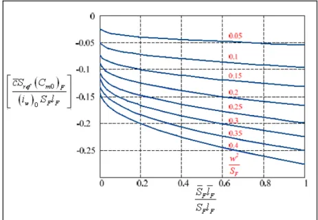
Figure 0.8 Fuselage effect on the zero lift pitching moment coefficient for the wing-body configuration (median position of the wing) ...28

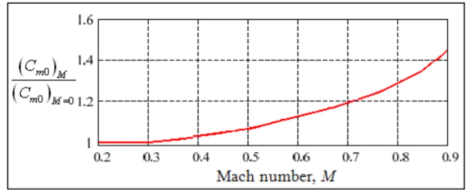
Figure 0.9 Effect of compressibility on the wing or wing-body zero lift pitching moment coefficient ...29

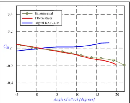
Figure 0.10 Pitching moment coefficient versus angle of attack estimated with FDerivatives and Digital DATCOM codes, compared with the experimental results provided by Thomas et al. (1957) ...33

Figure 0.11 Pitching moment coefficient versus angles of attack for WB and WBT configurations estimated with the FDerivatives code and compared with experimental results provided by Thomas et al. (1957) ...33

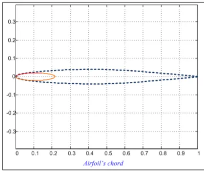
Figure 0.12 The ellipse that approximates the leading edge radius for the NACA 65A008 airfoil ...40

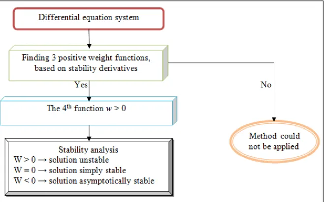
Figure 0.13 Logical diagram for the weight functions method ...44

Figure 0.14 Difference between Handling Qualities and Flying Qualities ...45

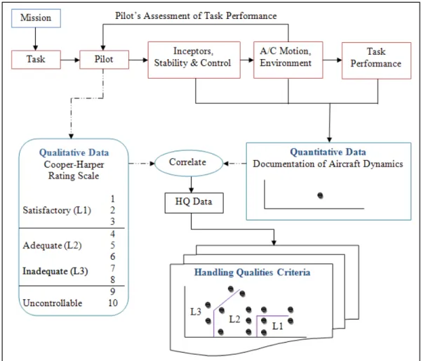
Figure 0.15 Diagram for developing Handling Qualities criteria ...46

Figure 0.16 Cooper-Harper rating scale ...49

Figure 0.17 Steps of the continuity algorithm ...52

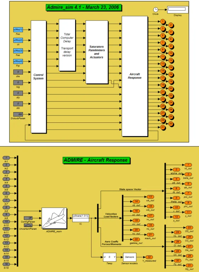
Figure 0.19 ADMIRE: Main graphical window simulation and the aircraft response ... 55

Figure 0.20 Angle of attack, elevon angle and thrust variation versus airspeed V, starting at the initial conditions presented in Table 5.4 for H = 20 m and M = 0.22 ... 64

Figure 0.21 Angle of attack, elevon angle and thrust variation versus airspeed V, starting at the initial conditions presented in Table 5.4 for H = 3000 m and M = 0.22 ... 66

Figure 0.22 Angle of attack, elevon angle and thrust variation versus airspeed V, starting at the initial conditions presented in Table 5.4 for H = 6000 m and M = 0.55 ... 68

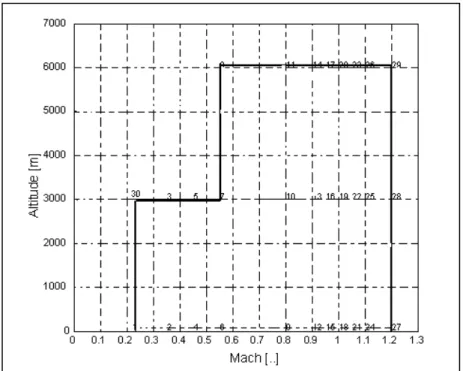
Figure 0.23 The flight envelope for HIRM aircraft stabilized with control laws ... 69

Figure 1.1 3D aircraft’s visualization in Digital DATCOM code ... 76

Figure 1.2 Drag coefficient due to elevator deflection results obtained with aircraft_name.xml command for A-380 aircraft, presented in the example given by Digital DATCOM code ... 76

Figure 1.3 Other modality to view the results for each coefficient in Digital DATCOM code ... 77

Figure 2.1 Three views of the Hawker 800XP aircraft ... 89

Figure 2.2 Logical scheme of FDerivatives code ... 91

Figure 2.3 Graphical interface of the FDerivatives code ... 93

Figure 2.4 Fuselage represented as a body of revolution ... 94

Figure 2.5 Lift coefficient distribution for the W configuration at Re = 3.49·106 ... 98

Figure 2.6 CL versus α (experimental versus calculated) for WB configuration... 99

Figure 2.7 Cm versus α (experimental and calculated), WB configuration ... 101

Figure 2.8 CLq and Cmq versus α, Hawker 800XP, WBT configuration ... 102

Figure 2.9 CDq versus α at the altitude H = 30 ft and q = 5 deg/s ... 102

Figure 2.10 versus α at the altitude H = 30 ft ... 103

Figure 2.11 versus α at the altitude H = 30 ft ... 104

lβ

C& yβ

Figure 2.12 versus α at the altitude H = 30 ft ...104

Figure 2.13 CL versus α at M = 0.4 ...105

Figure 2.14 CD versus α at M = 0.4 ...106

Figure 2.15 CL versus α at M = 0.5 ...106

Figure 2.16 CD versus α at M = 0.5 ...107

Figure 2.17 Cm versus α at Mach number = 0.3 ...108

Figure 2.18 Cyβ versus α at Mach number = 0.3 ...108

Figure 2.19 Clβ versus α at Mach number M = 0.3 ...109

Figure 2.20 Cnβ versus α at Mach number M = 0.3 ...109

Figure 2.21 Cyp versus α at Mach number M = 0.3 ...110

Figure 2.22 Cnp versus α at Mach number M = 0.3 ...110

Figure 2.23 Clp versus α at Mach number M = 0.3 ...111

Figure 2.24 Cnr versus α at Mach number M = 0.3 ...111

Figure 3.1 FDerivatives’ logical scheme ...118

Figure 3.2 Main window ...119

Figure 3.3 Wing and Canard parameters ...119

Figure 3.4 Fuselage parameters ...120

Figure 3.5 Vertical Tail parameters ...120

Figure 3.6 Wing geometry for X-31 model aircraft ...122

Figure 3.7 Twisted nonlinear wing for the X-31 aircraft ...123

Figure 3.8 Three-views of the X-31 model ...125

Figure 3.9 Lift coefficient variations with angle of attack ...127

Figure 3.10 Drag coefficient variations with angle of attack ...128

Figure 3.11 X–31 aircraft fuselage, modeled as a revolution body ...129

nβ

Figure 3.12 Pitching moment coefficient variations with angles of attack ... 130

Figure 3.13 Lift and pitch moment coefficients due to the pitch rate (CLq,Cmq ) versus the angle of attack ... 131

Figure 3.14 Yawing, side force and rolling moments due to the roll-rate derivatives’ variations with the angle of attack ... 132

Figure 3.15 Side force, yawing and rolling moments due to the sideslip angle derivatives’ variations with the angle of attack ... 133

Figure 3.16 Side force, rolling and yawing moment coefficients variation with angle of attack ... 135

Figure 3.17 Short-period response to phasor initial condition ... 138

Figure 3.18 Phugoid response to phasor initial condition ... 140

Figure 3.19 Short-period response to elevator step input ... 142

Figure 4.1 Coefficients ai and dj variation with the angle of attack ... 150

Figure 4.2 Weight functions chosen for longitudinal dynamics ... 151

Figure 4.3 Stability analyses with the weight functions method for different values of constant w4 as a function of angle of attack ... 152

Figure 4.4 The ci and bj coefficients’ variation with the angle of attack ... 154

Figure 4.5 Weight functions chosen for the lateral dynamics ... 155

Figure 4.6 Lateral-Directional stability analysis with the weight functions method for different values of constant w3 as a function of angle of attack ... 156

Figure 4.7 Root locus map longitudinal motion of the X-31 aircraft ... 158

Figure 4.8 Root locus map for lateral motion ... 159

Figure 5.1 The ai and dj coefficients’ variation with the angle of attack for Mach numbers M = 0.4 at altitude H = 3,000 m and M = 0.5 at H = 8,000 m ... 170

Figure 5.2 Weight functions w1long, w2long and w3long chosen for longitudinal dynamics at Mach numbers M = 0.4 and 0.5 corresponding to altitudes H = 3,000 and 8,000 m (left and right diagrams, respectively) ... 172

Figure 5.3 Stability analysis with the WFM for different values of constant w4long as a function of angle of attack for Mach number M = 0.4 ... 173

Figure 5.4 Stability analysis with the WFM for different values of constant w4long

as a function of angle of attack for Mach number M = 0.5 ...174 Figure 5.5 Weight functions variation with the angle of attack for lateral-directional

motion for M = 0.4 and H = 3,000 m (left) and M = 0.5 and H = 8,000 m (right) ...176 Figure 5.6 Lateral-directional stability analysis with the WFM for different values

of constant w4 as a function of the angle of attack for M = 0.4 ...177

Figure 5.7 Lateral-directional stability analysis with the WFM for different values of constant w4lat as a function of the angle of attack for M = 0.5 ...180

Figure 5.8 Root locus plot (Imaginary vs. Real eigenvalues) longitudinal motion

representation for M = 0.4 and 0.5 ...183 Figure 5.9 Root locus plot (Imaginary vs. Real eigenvalues) lateral directional

motion representation for M = 0.4 and 0.5 ...186 Figure 6.1 ADMIRE: Main graphical window simulation and Aircraft response ...194 Figure 6.2 Total weight function W for a complete range angle of attack/elevon

deflection, with a null canard deflection for longitudinal motion. ...202 Figure 6.3 Stability/instability fields for longitudinal motion using the Weight

Functions Method with w2 = 1 ...203

Figure 6.4 Equilibrium curves for elevon and canard deflection angles versus angle of attack ...204 Figure 6.5 Weight function W without/ with a control law at equilibrium for

longitudinal motion ...205 Figure 6.6 Total weight function W for a complete range of angle of attack/elevon

deflection, for lateral motion ...207 Figure 6.7 Equilibrium curves for elevon and rudder deflection angles versus

angle of attack ...208 Figure 6.8 Weight function W with and without a control law at equilibrium for

LIST OF ABREVIATIONS AND ACRRONYSMS

ADMIRE Aero-Data Model in Research Environment

AG Action Group

AOA Angle of attack

AVT Applied Vehicle Technology

CRIAQ Consortium for Research and Innovation in Aerospace in Quebec

DLR German Aerospace Center (Deutsches Zentrum fűr Luft-und Raumfahrt e.V.) DNW–NWB Low–Speed Wind Tunnel of the German–Dutch Wind Tunnels

GARTEUR Group for Aeronautical Research and Technology in EURope FM Flight Mechanics

FOI Swedish Defence Research Agency HIRM High Incidence Research Aircraft Model HQM Handling Qualities Method NATO North Atlantic Treaty Organization

LARCASE Laboratory of Research in Active Controls, Aeroservoelasticity and Avionics PIO Pilot-Involved (Pilot-Induced) ( Pilot-In-the-loop) Oscillations

RTO Research and Technology Organization SAAB Saab AB

LIST OF SYMBOLS

b Wing span

c MAC (Mean Aerodynamic Chord) CA Axial-force coefficient

CD Drag coefficient

CDα Drag due to the angle of attack derivative

CDq Drag due to the pitch rate derivative Dα

C _ Drag due to the angle of attack rate derivative

(CH)A Control-surface hinge moment derivative due to angle of attack (CH)D Control-surface hinge moment derivative due to control deflection cL Local airfoil section lift coefficient

CL Lift coefficient

(CLA)D Lift-curve slope of the deflected, translated surface cLmax Maximum airfoil section lift coefficient

CLmax Wing maximum lift–coefficient

CLα Lift due to the angle of attack derivative

CLq Lift due to the pitch rate derivative mα

C _& Lift due to the angle of attack rate derivative Cm Pitching moment coefficient

Cm0 Zero pitching moment coefficient

Cmα Static longitudinal stability moment with respect to the angle of attack

derivative

mα

C & Pitching moment due to the angle of attack rate derivative

CN Normal-force coefficient

Clp Rolling moment due to the roll rate derivative

Clr Rolling moment due to the yaw rate derivative

Clβ Rolling moment due to the sideslip angle derivative lβ

C_ Rolling moment due to the sideslip angle rate derivative Cnp Yawing moment due to the roll rate derivative

Cnr Yawing moment due to the yaw rate derivative

Cnβ Yawing moment due to the sideslip angle derivative nβ

C _ Yawing moment due to the sideslip angle rate derivative CT Tangential force coefficient

Cyp Side force due to the roll rate derivative

Cyr Side force due to the yaw rate derivative

Cyβ Side force due to the sideslip angle derivative yβ

C _ Side force due to the sideslip angle rate derivative DELTA Control-surface steamwise deflection angle

DELTAT Trimmed control-surface steamwise deflection angle D(CDI) Incremental induced-drag coefficient due to flap deflection

D(CD MIN) Incremental minimum drag coefficient due to control or flap deflection

D(CL) Incremental lift coefficient in the linear-lift angle of attack range due to deflection of control surface

D(CM) Incremental pitching moment coefficient due to control surface deflection valid in the linear lift angle of attack

fk Functions used for weight functions method

g Gravity acceleration constant H Altitude

Ix, Iy, Iz Moment of inertia about the X, Y and Z body axes, respectively

Ixz Product of inertia

Ixy x-y body axis product of inertia

lβ Rolling moment due to the sideslip angle derivative

lαβ Rolling moment due to the roll rate derivative and alpha derivative

lαδa Rolling moment due to the aileron derivative and alpha derivative

lδa Rolling moment due to the aileron derivative

lδr Rolling moment due to the rudder derivative

lr Rolling moment due to the yaw rate derivative

lp Rolling moment due to the roll rate derivative

Lp Rolling moment due to roll rate

Lr Rolling moment due to yaw rate

Lβ Rolling moment due to sideslip

Lδ Roll control derivative

m Aircraft mass

M Mach number

Mq Pitching moment due to pitch rate

Mα Pitching moment due to incidence α

M_ Pitching moment due to the rate of change of the incidence Mδ Pitching moment due to flaps deflection

nβ Yawing moment due to the sideslip angle derivative

nαp Yawing moment due to the roll rate derivative and alpha derivative

nαδa Yawing moment due to the aileron derivative and alpha derivative

nδa Yawing moment due to the aileron derivative

nδr Yawing moment due to the rudder derivative

nr Yawing moment due to the yaw rate derivative

np Yawing moment due to the roll rate derivative

Np Yawing moment due to roll rate

Nr Yawing moment due to yaw rate

Nβ Yawing moment due to sideslip

Nδ Yawing moment due to flap deflection

p Roll rate

p, q, r Angular rates about the X, Y and Z body axes, respectively

p, q, r   Time rate of change of p, q, r

q Pitch rate

q/q∞ Dynamic pressure ratio

q∞ Dynamic pressure

r Yaw rate

S Wing area

T Thrust Tp Phugoid mode period

u Forward velocity

u Time rate of change of u V Airspeed

wk Weight functions

W Total Weight functions

xCG Distance between the centre of gravity of the aircraft and the quarter–chord

point of wing MAC, parallel to MAC, positive for CG aft of MAC xeng x-position of the engine's center of gravity

xk Unknown of the system used for weight functions method

XCP Distance between the aircraft moment reference centre and the centre of pressure divided by the longitudinal reference length

Xu Drag increment with increased speed

Xα Drag due to incidence

Xδ Drag due to flap deflection

yβ Side force due to the sideslip angle derivative

yδa Side force due to the aileron derivative

yδr Side force due to the rudder derivative

yr Side force due to the yaw rate derivative

yp Side force due to the roll rate derivative

Yp Side force due to roll rate

Yr Side force due to yaw rate

Yδ Side force control derivative

Zq Lift due to pitch rate

Zu Lift increment due to speed increment

Zα Lift due to incidence α

Z_ Lift due to the rate of change of incidence Zδ Lift due to flap deflection

α Angle of attack

α,β,θ_   Time rate of change of α, β, θ

β Sideslip angle

δ Control deflection

δa Aileron deflection

δc Canard deflection

δe Elevator deflection

δLEi Wing, leading-edge inner flaps

δLEo Wing, leading-edge outer flaps

δTE Wing, trailing-edge flaps

δr Rudder deflection

ΛLE Quarter–chord sweep angle at Leading Edge

κLs Stall factor in the relation for maximum lift coefficient

κLΛ Sweep factor in the relation for maximum lift coefficient

κLθ Twist factor in the relation for maximum lift coefficient

λp Phugoid eigenvalues

ɸ Roll angle

Φ Bank angle

ωnsp Short-period modal damping

ωnp Phugoid modal damping

θ Total twist (geometrical and aerodynamic)

θ Pitch angle

ψ Heading angle

ζsp Short-period natural frequency

ζp Phugoid natural frequency

Index

B Body (Fuselage)

CG Centre of Gravity

LE Leading Edge

H Horizontal Tail

k Number of weight functions

p Phugoid

sp Short period

TE Trailing Edge

V Vertical Tail

WB Wing Body

WBH Wing Body Horizontal Tail

INTRODUCTION

For airplanes, one of the main concerns is that the vehicle is easily controllable and maneuverable. Two different aspects are important: controllability and stability, concepts which are not equivalent. A high number of airplanes considered excellent in terms of their characteristics (dimensions, weights and performances) show a slight lateral instability called divergence spiral. Instability is no longer a problem thanks to the fly–by–wire system which replaces the conventional manual flight control. The automatic signals sent by the aircraft's computers allows to perform functions without needing the pilot's input, as in systems that automatically help stabilize the aircraft.

Today, generation of mathematical models needed to represent the various dynamics phenomena are very important in the aerospace field. Such mathematical models are conceived in many disciplines related to aerospace engineering. Major aerospace companies have developed their own codes to estimate the aerodynamics characteristics and aircraft stability in conceptual phase.

In parallel, universities have developed various codes for educational and research purpose. At LARCASE laboratory, where the projects are focused mainly in aeronautical field, a code called FDerivatives was dedicated to the analytical and numerical calculations of the aerodynamics coefficients and their corresponding stability derivatives. This code is written in MATLAB and has a user friendly graphical interface. Strongly linked to the aircraft geometry and flight conditions, the aerodynamic derivatives are needed for its stability and control analysis. Given the complexity and the scope of this project, the research was performed on the aircraft flying in the subsonic regime. Presagis gave the « Best Simulation Award » to the LARCASE laboratory for FDerivatives and data FLSIM applications.

This code can be used as a design tool, and new methods for aircraft's analysis have been added, to be able to complete the aim of this thesis. The weight functions method was applied

to study the stability and a numerical application of the continuity algorithm is presented to improve the flight envelope for minimum airspeeds.

Figure 0.1 The main methods used for aircraft analysis

This research thesis is part of two projects. The first project was initiated by CAE Inc. and the Consortium for Research and Innovation in Aerospace in Quebec (CRIAQ) and the second project was funded by NATO in the frame of the NATO RTO AVT–161 program,

«Assessment of Stability and Control Prediction Methods for NATO Air and Sea Vehicles ». The latter project was awarded the « RTO Scientific Achievement Award 2012 », the most prestigious award that has been offered to the AVT-161 NATO research team.

Three aircraft models were analyzed in this paper:

• The Hawker 800XP, a midsize twin–engine corporate aircraft with low swept–back one–piece wing, a high tail plane and rear–mounted engines;

Aircraft's geometry

FDerivatives code: calculation of aerodynamic coefficients and their derivatives (Hawker 800XP and X-31)

Weight Functions Method: stability analysis • stable aircraft (Hawker 800XP and X-31) • unstable aircraft (HIRM) - added control law

Continuity algorithm: improve the flight envelope using a control law (HIRM)

• The X–31 aircraft, designed to break the « stall barrier », which allows it to fly at angles of attack that would typically cause an aircraft to stall resulting in loss of control; and

• The High Incidence Research Model (HIRM) of a generic fighter aircraft implemented in Aero-Data Model In Research Environment (ADMIRE) code, developed by the Swedish Defense Research Agency.

Four of the five journal papers presented in this thesis use the in-house results obtained with FDerivatives code. The first two papers were written in collaboration with my colleagues at the LARCASE laboratory. My contributions as main author, as well as the contributions of colleagues to each article, are specified in the Objectives and Originality section. As Ph.D. advisor, Dr. Botez is the co–author of these papers.

In the first paper, the aerodynamics and stability coefficients are estimated based for the Hawker 800XP, a mid-size corporate aircraft, using the new in-house FDerivatives code. These coefficients were further validated with the geometrical and experimental flight test data provided by CAE Inc.

The second paper was also realized by use of the same in-house code, but for a different aircraft configuration. The X–31 aircraft is a delta-wing configuration that was tested in the Low–Speed Wind Tunnel of the German–Dutch Wind Tunnels (DNW–NWB). By taking into account a minimum number of geometrical parameters delivered by German Aerospace Center (DLR), the remaining geometrical data were calculated to complete the database of the aircraft’s geometry. The aerodynamics and their stability coefficients, as well as the total side force, rolling and yawing moments’ coefficients were validated with wing tunnel test data. The longitudinal behavior of the aircraft about the pitch–axis reference frame was also analyzed.

We began with a code based on the geometrical parameters of an airplane, and built on that with a new method called the weight functions method. This method was applied for

longitudinal and lateral–directional dynamics studies in the last three papers. This method extends the FDerivatives code so that it can produce a complex analysis of aircraft stability, as a design tool, completed with the continuity algorithm used to estimate flight envelope minimum airspeeds.

The development of a new interface that can unify FDerivatives code with the weight functions method and a continuity algorithm could be a future project at LARCASE. Before embarking on this new project it will be necessary to validate how to choose the weight functions for similar aircraft configurations (classical configuration wing-body-tail, as in the Hawker 800XP, a wing-delta configuration, as in the X-31, and a wing-delta configuration equipped with thrust vectoring capability, as with the HIRM). Therefore, a minimum of three different aircraft will analyzed with the weight functions method.

The weight functions method presented here is similar to the Lyapunov method, except for how the weight functions are defined. In the Lyapunov method the functions are chosen simultaneously, while for the weight functions method each weight function is selected step by step. Numerical results are presented in the last three papers.

The continuity algorithm is described in this thesis as the last step in our analysis, and numerical results are presented for HIRM aircraft in order to estimate the minimum airspeeds of the flight envelope for the model stabilized by using the control law.

This thesis is organized as follows: A literature review is presented in Chapter 1 after a detailed Introduction. A introduction to the first paper and to the FDerivatives code is provided in Chapter 2, including the detailed results and description of the FDerivatives code for the Hawker 800 XP configuration. The second paper is fully presented in Chapter 3. The weight function and the handling qualities methods are introduced and presented in Chapter 4 (for the X-31 aircraft), Chapter 5 (for the Hawker 800 XP) and Chapter 6 (for HIRM model aircraft). General conclusions and further work recommendations complete this thesis.

The following sections explain the objectives and the originality of the proposed work and the applied theory is also summarized. A detailed introduction to the FDerivatives code, how it works and its structure is presented. Stability analysis is covered in Section 0.5, where the theory is developed for the weight functions method, the handling qualities method and the continuity algorithm, with numerical results applied to HIRM aircraft.

0.1 Objectives and originality

The main objective of this thesis is to perform a more complete analysis of an aircraft in subsonic regime as a design tool, based on geometrical parameters. Its originality lies in the methods chosen to analyze the stability of three real aircraft, sustained with numerical results. In order to accomplish this task, this research treats three categories:

• The new in–house FDerivatives code, developed at LARCASE laboratory, designed to calculate the aerodynamic coefficient values and their derivatives. The results have been validated numerically for two different aircraft configurations: the Hawker 800XP and X-31 aircraft.

• The Weight Functions Method (WFM) is used as a design tool to determine an aircraft’s stability. The method was applied on the Hawker 800XP, the X-31 and a High Incidence Research Aircraft Model (HIRM) aircraft.

• A continuity algorithm is used to estimate the minimum airspeeds for longitudinal dynamics of the HIRM aircraft, stabilized with the control law.

To achieve this goal, the flight test data provided by CAE Inc for the Hawker 800XP and the experimental results provided by the Low–Speed Wind Tunnel of the German–Dutch Wind Tunnels (DNW–NWB) for the X–31 model have been invaluable. With their data, along with the real airfoils’ coordinates, the FDerivatives code could be validated. The High Incidence Research Aircraft Model (HIRM) developed by the Swedish Defense Research Agency and implemented in Aero-Data Model In Research Environment (ADMIRE) code was used to validate the WFM and the continuity algorithm. The flight configurations were selected because they are among the flight conditions for Cat. II Pilot Induced Oscillation (PIO)

criteria validation, performed on the FOI aircraft model presented in the PIO Handbook by the Group for Aeronautical Research and Technology in Europe, Flight Mechanics/Action Group 12.

The first step was to help to define and complete the FDerivatives code, conceived and developed to calculate the aerodynamic coefficients and static/dynamic stability derivatives of an aircraft in subsonic regime, based on its geometrical data. FDerivatives is an implementation in MATLAB of the DATCOM method, improved for estimating the pitching moment coefficient, the lift curve slope, and for the calculus of the aerodynamic parameters for airfoils specified by NACA. This will be detailed in Section 0.4, with the code description and its improvements.

The first model implemented and tested in FDerivatives code was the geometry of a Hawker 800XP, thoroughly checked and verified for missing data (such as airfoils, fuselage coordinates, among others). Each function contained in the DATCOM method was then implemented in MATLAB with the relevant improvements. The task required teamwork, and a large part of the implementation of the methods in FDerivatives code was accomplished by Mr. Dumitru Popescu.

The checking and completing of the geometry in order to implement it in Digital DATCOM and validate its first phase with flight test data was part of my work. Once the geometry was validated I switched to the MATLAB code. I first verified all the functions written earlier by my team, and then I continued to implement the derivatives functions regarding the sideslip, the roll rate and the pitch moment coefficient.

While the FDerivatives code was being completed for a typical wing-body-tail configuration, the canard model was implemented. The graphical interface was radically changed; this change can be seen in the second journal publication. The results were validated using the X– 31 aircraft geometry and the wind tunnel experimental data for Mach number 0.18 at Sea

Level. This model was also tested in Digital DATCOM, where the wing was implemented as a horizontal tail and the canard as the wing parameters.

Once the code was completed and validated for two real aircraft, with different configurations, the second step was to choose and apply a new stability method called the Weight Functions Method. This new method replaces the classical Lyapunov stability criterion based on finding a Lyapunov function. Finding a Lyapunov function is not simple task and it is not always guaranteed. The Lyapunov method is very useful, however, when the linearization around the point of equilibrium leads to a matrix of evolution with eigenvalues having zero real parts.

The difference between these two methods is that the WFM finds one function at a time, with their number equal to the number of the first-order differential equations. The WFM’s basic principle is to find three positive weight functions for a system with four first-order differential equations, where the fourth weight function is a constant, imposed by the user. Aircraft stability is determined from the sign of the total weight function; this sign should be negative for a stable aircraft. The Root Locus method was used to validate this new method.

The first two aircraft models were stable, and so a third, nonlinear model was used. For HIRM aircraft the WFM was applied to the original aerodynamics model implemented in ADMIRE code, as well as for the model stabilized with control laws, defined for longitudinal and lateral motions. Starting with its flight envelope, which has a non-typical shape, the continuity algorithm was chosen to improve this envelope for a HIRM model stabilized with the control law.

0.2 Background theory on aircraft modelling

The theoretical concepts on which the subsequent chapters are based are next described. An aircraft is represented in Figure 0.2 in the body axis system, which is fixed in the aircraft’s

centre of gravity. The x– axis is positive forward through the nose, the y– axis is positive out through the right wing and the z– axis is positive upward.

Figure 0.2 Body axis system of the aircraft

Table 0.1 presents the applied forces and moments, as well as the angular velocities and positions found in the reference axis system.

Table 0.1 Notations for speeds, positions, moments of inertia, forces and moments in an aircraft’s reference axis

Axis Linear speed Angular speed Angular position Moment of inertia Moment applied Force applied x u p roll rate φ roll angle Ix roll inertia L X y v q pitch rate θ pitch angle Iy pitch inertia M Y z w r yaw rate ψ yaw angle Iz yaw inertia N Z

The six equations of forces and moments (Etkin et al., 1996) used to analyze the Hawker 800XP and X-31 aircrafts are given by eq.(0.1):

(

)

(

)

(

)

(

)

(

)

(

)

(

)

(

)

(

)

Three other equations are required to relate the angular rates p, q and r to the Euler angles: φ,

θ and ψ (see eq.(0.2)).

sin

cos cos sin

cos cos sin

p q r φ ψ θ θ φ ψ θ φ ψ φ θ θ φ = − = + = −    _   (0.2)

The Euler rates are defined in eq.(0.3)

(

)

sin tan cos tan

cos sin

sin cos sec

p q r q r q r φ φ θ φ θ θ φ φ ψ φ φ θ = + + = − = +    (0.3)

The model described by eqs (0.1), (0.2) and (0.3) was used to study the stability of two different aircraft configurations, for the Hawker 800XP and the X31.

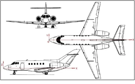
The first aircraft studied in this paper is the Hawker 800XP, a midsize twin–engine corporate aircraft with low swept–back one–piece wings, a high tailplane and rear–mounted engines, for which the maximum Mach number is equal to 0.9. This aircraft operates in the subsonic and transonic regimes. Three views of the Hawker 800XP aircraft are represented in the OXYZ reference system (Figure 0.3).

Figure 0.3 Three views of the Hawker 800XP aircraft

Table 0.2 Hawker 800XP wing characteristics

Airfoils Root section NACA 4420

Tip section NACA 4412

Taper ratio 2.5 Aspect ratio 10.05 Span 15 [ft] Area 22.39 [ft2] Root chord 2.143 [ft] MAC 1.592 [ft] Tip chord 0.8572 [ft] Geometrical twist –3.50 Aerodynamical twist –3.40 Sweepback angle of leading edge 120

Dihedral angle 20

Reynolds number 3490000

The study proposed in the present thesis is mainly based on the geometry of tested aircraft. Because the number of the parameters defining the inputs to estimate the aerodynamic and

stability coefficients in FDerivatives code is very large, it was sometimes necessary to estimate the missing geometrical data. These parameters are detailed in the next section.

The X–31 aircraft, the second aircraft analyzed, was designed to break the « stall barrier », allowing it to fly at angles of attack that would typically cause an aircraft to stall resulting in loss of control. The X–31 employs thrust vectoring paddles which are placed in the jet exhaust, allowing the aircraft’s aerodynamic surfaces to maintain their control at very high angles. For its control, the aircraft has a small canard, a single vertical tail with a conventional rudder, and wing leading–edge and trailing–edge flaps.

The X–31 aircraft also uses computer controlled canard wings to stabilize the aircraft at high angles of attack. The stall angle at low Mach numbers is α = 300. The X–31 model geometry (Henne et al., 2005) was given by the DLR, at the scale 1:5.6 (Table 0.3) at the AVT–161 meeting.

Table 0.3 Geometrical parameters

Fuselage length 1.725 m Wing span 1.0 m Wing Mean Aerodynamic Chord (MAC) 0.51818 m Wing reference area 0.3984 m2 Wing sweep angle, inboard 57 deg Wing sweep angle, outboard 45 deg Canard span 0.36342 m Canard reference area 0.04155 m2 Canard sweep angle 45 deg Vertical Tail reference area 0.0666 m2 Vertical Tail sweep angle 58 deg

The main part of the X–31 model is a wing–fuselage section with eight servo-motors for changing the angles of the canard (δc), the wing Leading–Edge inner/outer flaps (δLei / δLEo), wing Trailing–Edge flaps (δTE) and the rudder (δr) (Rein et al., 2008). The variation of these angles, for each control surface, is given as:

o Canard: –700 _{≤ δ}

c ≤ 200,

o Wing inner Leading-Edge flaps: –700 ≤ δLEi ≤ 00, o Wing outer Leading-Edge flaps: –400 ≤ δLEo ≤ 00, o Wing Trailing-Edge flaps: –300 ≤ δTE ≤ 300, o Rudder: –300 ≤ δr ≤ 300.

The wing parameters were introduced in Digital DATCOM for the horizontal tail and the canard as a wing.

The third model in this study is the HIRM (High Incidence Research Model) (Admirer4p1), (Lars et al., 2005), (Terlouw, 1996) of a generic fighter aircraft. This aircraft model has an envelope defined by a Mach number between 0.15 and 0.5 and altitude of between 100 and 20,000 ft for the following angles: the angle of attack α = [-10 to 30] degrees, sideslip angle β = [-10 to 10] degrees, elevon angle δe = [-30 to 30] degrees, canard angle δc = [-55 to 25] degrees, and rudder angle δr = [-30 to 30] degrees.

The aerodynamics coefficients were obtained based on wind tunnel and flight tests (Admirer4p1) for a model « ... originally designed to investigate flight at high angles of

attack ... but [that] does not include compressibility effects resulting from high subsonic speeds. » (Terlouw, 1996, p 21).

Figure 0.4 Body axes system of an HIRM aircraft

Table 0.4 Summary of the HIRM aircraft's geometrical data, along with aircraft mass and mass distribution data

Parameters Numerical values [Units]

Wing area S 45 m2

Wing span b 10 m

Wing Mean Aerodynamic Chord c 5.2 m

Mass m 9100 kg

x-body axis moment of inertia Ix 21000 kgm2

y-body axis moment of inertia Iy 81000 kgm2

z-body axis moment of inertia Iz 101000 kgm2

xz-body axis product of inertia Ixz 2500 kgm2

zeng -0.15 m

xcg 0.25c

The HIRM aircraft was evaluated (see Figure 0.4 and Table 0.4) based on the nonlinear system of equations given by eq.(0.4):

(

)

(

)

(

)

(

)

(

)

(

)

(

)

(

)

(

)

(

)

(

)

₍

₎

(

)

(

)

(

)

(

)

(

)

cos cos cos cos sin sin cos

cos sin cos sin sin

sin cos sin sin sin cos cos

sin sin cos cos sin

sin cos sin cos cos

r q r q r x u v w y u v w z u v w φ φ θ θ φ φ φ φ ψ θ ψ θ ψ θ φ ψ φ ψ θ φ ψ φ ψ θ ψ θ φ ψ φ ψ θ φ ψ φ θ θ φ θ φ        +  = − + = = + − + + + = + + + + − = − + +                         (0.4) 0.3 DATCOM method

The aircraft geometrical parameters are: wing span, Mean Aerodynamic Chord (MAC), sweep back angle of the leading edge, reference surface, weights, thrust, speeds (minimum control speed on the ground (VMC Ground), take–off safety speed (V2) and landing reference speed or threshold crossing speed (VREF), length, height, position of the gravitational centre, position and number of the engines, among numerous others.

The required inputs are estimated as a function of the airfoils’ coordinates, while the aircraft geometrical data is given in 3D coordinates.

A. Digital DATCOM limitations (Finck et al., 1978)

An aircraft’s stability is measured in terms of its derivatives - the rate of change of one variable with respect to another variable. The DATCOM method, implemented in FORTRAN and called the Digital DATCOM code presents several operational limitations (Finck et al., 1978), (Williams et al., 1979a) (see Table 0.5).

• « The forward lifting surface is always input as the wing and the aft lifting surface as the horizontal tail. This convention is used regardless of the nature of the configuration.

• Twin vertical tail methods are only applicable to lateral stability parameters at subsonic speeds.

• Airfoil section characteristics are assumed to be constant across the airfoil span, or as an average for the panel. Inboard and outboard panels of a cranked or double–delta planform can have their individual panel leading edge radii and maximum thickness ratios specified separately.

• If airfoil sections are simultaneously specified for the same aerodynamic surface by an NACA designation and by coordinates, the coordinate information will take precedence.

• Jet and propeller power effects are only applied to the longitudinal stability parameters at subsonic speeds. Jet and propeller power effects cannot be applied simultaneously.

• Ground effect methods are only applicable to longitudinal stability parameters at subsonic speeds. • Only one high lift or control device can be analyzed at a

time. The effect of high lift and control devices on downwash is not calculated. The effects of multiple devices can be calculated by using the experimental data input option to supply the effects of one device and allowing Digital DATCOM to calculate the incremental effects of the second device.

• Jet flaps are considered to be symmetrical high lift and control devices. The methods are only applicable to the longitudinal stability parameters at subsonic speeds. • The program uses the input namelist names to define

the configuration components to be synthesized. For example, the presence of namelist HTPLNF causes

Digital DATCOM to assume that the configuration has a horizontal tail. » (Finck et al., 1978, p 17)

Table 0.5 DATCOM method limitations Source: Finck et al. (1978, p 6)

B. Classical aircraft configurations Wing – Body – Tail and Canard

This DATCOM reference treats the classical body–wing–tail stability and geometry including control effectiveness for a variety of high–lift/control devices. The outputs for the high–lift/control devices are usually expressed in terms of incremental effects due to control surface deflections.

Digital DATCOM code is applied to the classical aircraft, including canard configurations, in order to estimate the following characteristics:

 Static stability characteristics. In Digital DATCOM, where the semi–empirical DATCOM methods are computed, the longitudinal and the lateral–directional stability derivatives have been calculated in the stability axis system. The outputs are: the normal force CN and the axial force CA coefficients, the lift, drag and moment coefficients CL,

CD, and Cm ,as well as their corresponding longitudinal derivatives CLα, Cmα, Cyβ, Cnβ and

Clβ.

 Dynamic stability lift, pitch, roll and yaw derivatives CLq, Cmq, Clp, Cnp, Clr, Cnr, , and .

 High–lift and control characteristics including jet flaps, split, plain, single slotted, double slotted, fowler and leading edge flaps and slats, trailing edge flap controls and spoilers.

 Trim data, which can be calculated only for subsonic speeds, where Cm = 0. The trim option is available for the first mode configurations, as they have a trim control device on the wing or horizontal tail, and for the second mode configurations, where the horizontal tail is all–movable.

0.4 FDerivatives code: Description and improvements

With its projects focused mainly in the aerospace field, LARCASE identified the need to develop a new code for educational and research purposes. This new code, called FDerivatives, is dedicated to the analytical and numerical calculation of the aerodynamics

coefficients and their corresponding stability derivatives. FDerivatives is written in MATLAB and has a user-friendly graphical interface. Strongly linked to aircraft geometry and flight conditions, the aerodynamic coefficients and derivatives are needed for aircraft stability and control analysis. Given the complexity and scope of this project, the research was limited to aircraft flying in the subsonic regime.

C. Description of the FDerivatives code

The model implemented in the new FDerivatives code is based on the methodology used in the DATCOM procedure (Williams et al., 1979a) for calculating the aerodynamic coefficients and their stability derivatives for an aircraft. The main advantage of this new code is the estimation of the lift, drag and moment coefficients and their corresponding stability derivatives by use of relatively few aircraft geometrical data: area, aspect ratio, taper ratio and sweepback angle for the wing and for the horizontal and vertical tails.In addition, the airfoils for the wing, the horizontal and vertical tails, as well as the fuselage and nacelle parameters, are designed in a three–dimensional plane.

A logical block diagram is presented in Figure 0.5, which shows how the code works, as a function of the chosen configuration. The methods presented as a function of Mach number for a WBT configuration are also given for the other two configurations WB and W in the same four regimes: low-speed, subsonic, transonic and supersonic. The graphical interface is designed to allow the user to select the desired configuration for the calculation of the aerodynamic coefficients and stability derivatives.

Figure 0.5 Logical diagram of the new FDerivatives code

In the FDerivatives code, the Reynolds number and the airflow speed over the aircraft are calculated by considering a theoretical atmospheric model such as the model defined by the International Civil Aviation Organization (ICAO). This model is an ideal one, in which the atmosphere is divided into seven different layers, with a linear distribution of temperature.

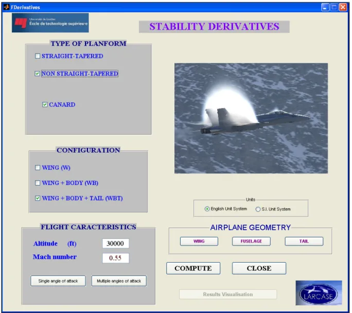
The main window of the graphical interface is presented in Figure 0.6. The flight characteristics (altitude, Mach number and angle of attack), the type of the planform (straight–tapered or non-straight–tapered wing or canard) and the configuration, ,Wing, Wing–Body or Wing–Body–Tail must be defined before the outputs can be calculated.

Figure 0.6 Main window of the graphical interface for the FDerivatives code

Two types of input data are needed for the program. The first set are the geometrical parameters defining the various components of an aircraft’s wing, fuselage and nacelles, horizontal and vertical tails. The number of parameters is dictated by the geometry of each element, and the input done manually, through the « Airplane Geometry » graphic of the Stability Derivatives’ main window software. The second set of data is composed of the coordinates of contour points, taken at representative locations on the surfaces, as well as contact points of the contour of the fuselage and nacelles. A function is responsible for their automatic import from Excel spreadsheets. The input parameters needed to calculate the aerodynamic coefficients and their stability derivatives are described in Tables 0.6 and 0.7.

The input data for the fuselage and nacelles are coordinates taken as contour points in two perpendicular planes: the horizontal plane parallel to the axis of reference of the aircraft and the vertical plane containing the axis of symmetry. These data are used for calculating the geometrical parameters required for asymmetric fuselage modeling.

Table 0.6 Inputs for Wing/Canard and Horizontal/Vertical Tail’s geometry Aspect ratio – AW = b2 /SW

Taper ratio – λW

Reference area [ft2] – SW

Quarter chord sweep angle [0] – (Λc/4)W Dihedral angle [0] - ΓW

Airfoils given for Root, MAC and Tip section in 3D coordinates

Parameters to estimate the Wing/Canard and Horizontal/Vertical Tail’s geometry Span [ft] – bW

Root chord [ft] – crW Tip chord [ft] – ctW

Mean Aerodynamic Chord [ft] – c

Lateral position of the MAC [ft]

Sweepback angle at leading edge [0] – ΛLE Sweepback angle at 25% chord line [0] – Λc/4 Sweepback angle at 50% chord line [0] – Λc/2 Sweepback angle at trailing edge [0] – ΛTE

Twist of tip respect to root, negative for washout [0] – θ Span of the exposed surface [ft] – beW

Root chord of exposed surface [ft] – cRe Tip chord of exposed surface [ft] – cTe Area of exposed surface [ft2] – (Se)W

Sweepback angle of the exposed surface [0] – Λ(LE)We Aspect ratio of exposed surface – AWe

Mean Aerodynamic Chord of the exposed surface [ft] – c _We

Lateral position of the MAC for exposed surface [ft] Twist of tip respect to root, for exposed surface [0] – θWe

Sweepback angle at leading edge for exposed surface [0] – Λ(LE)We Sweepback angle at 25% chord line for exposed surface [0] – Λ(c/4)We Sweepback angle at 50% chord line for exposed surface [0] – Λ(c/2)We Sweepback angle at trailing edge for exposed surface [0] – Λ(TE)We

Table 0.7 Inputs for fuselage parameters Body section – circular or elliptical

Nose type – cone or ogive

Forebody – conical or parabolic profile After body – conical or parabolic profile Body length [ft]

Position of the gravity centre on x-axis [ft] Position of the gravity centre on z-axis [ft] Body coordinates in XOY plane and XOZ plane Number of nacelles

Position Xo of the nacelle on x-axis [ft] Nacelle length [ft] -

Nacelle coordinates in XOY plane and XOZ plane

Other usefully dimensions

Exposed wetted area of body (isolated body minus surface area covered by the wing at wing-body junction) [ft2] – (Ss)e

Maximum fuselage diameter [ft] – d Maximum cross-section area – SB Lateral fuselage area – SSe

Body base area – Sbase Body side area – SbS

Total body volume – VB

Wetted or surface body area excluding base area of wing at root – Ss

The new code is organized into several sub-directories, all grouped in a root directory called FDerivatives_Matlab. Figure 0.7 shows the subdirectories and part of the contents of the root directory of the code. Apart from sub-directories, this directory contains all the main MATLAB functions: the FDerivatives.m function which manages the main graphics window and the rest of the functions for calculating the aerodynamic coefficients and their stability derivatives.

Figure 0.7 Root directory of the FDerivatives code The subdirectories and their destinations are described below:

• Database folder contains all the text files containing the data obtained from the chart scanning;

• Geometry folder keeps all the functions, is of secondary in importance in the algorithm’s operation;

• Input_Data folder is reserved for the parameters from the Excel data files required for the derivative calculation;

• Output folder represents the destination of the results at the end of program; and • Photos folder stores the pictures, logos and designs used by the graphical interface.

In addition to the inputs of the Digital DATCOM code, FDerivatives code takes into account the aerodynamic contributions of nacelles, without any restrictions on their position relative to the fuselage or wing. However, for a given aircraft, the code considers only an even number of nacelles, attached either to the fuselage or to the wings, with no possibility of a combined arrangement (as in the Lockheed L1011 aircraft, for example, where the contribution of the third engine’s nacelle, located on the dorsal part of the fuselage, is neglected).

For canard configuration, the wing is treated as the horizontal tail, while the canard is treated as the main wing. Neither the FDerivatives nor the Digital DATCOM code treat aircraft with three lifting surfaces, as DATCOM’s methods lack that capability. By three lifting surfaces, we refer here to airplanes equipped with two main wings, one above the other (the biplane model), and aircraft with a main conventional wing, horizontal tail located at the rear and a canard in addition. The codes do not treat the winglets or vertical stabilizers with more than two lifting surfaces.

D. Improvements of the FDerivatives code to Digital DATCOM

From a methodological point of view, the new methods implemented in FDerivatives code and presented in this thesis discus a qualitative approach. These methods promote the

approaches that we have used to produce a modern, user-friendly tool for calculating aerodynamic coefficients and stability derivatives.

For the main functions, a general model to implement all the calculation methods was developed and used in the new code. This model allows for easy replacement of the methodologies implemented, including adding new methods, and simplifies the debugging process.

Compared to Digital DATCOM’s applicability limits, the FDerivatives code adds several enhancements. The possibilities of calculating have been extended to wings with variable airfoils along the span and negative sweepback. Different approaches to calculate the drag and pitching moment of the aircraft allow the results for the drag coefficient to be refined, and significantly improve the coefficient of pitching moment results. The improvements added to FDerivatives code versus Digital DATCOM code are detailed in the paragraphs that follow.

D.1. Pitching moment estimation for Wing-Body configuration in Digital DATCOM code

The solution presented and used in Digital DATCOM code for the calculus of the pitching moment estimated as a function of the angle of attack for the WB configuration is presented in this section. The equation implemented in the code is:

( )

( ) ( )

m m _WB m _L m _D

C ₌ C ₊ C ₊ C (0.5)

where

(Cm0)WB is the zero lift pitching moment coefficient for the WB configuration

(Cm)L is the moment coefficient given by the lift force as a function of the angle of attack

(Cm)D is the moment coefficient given by the drag force as a function of the angle of attack