Application of the Proper Generalized Decomposition to Solve MagnetoElectric Problem
Texte intégral
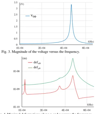
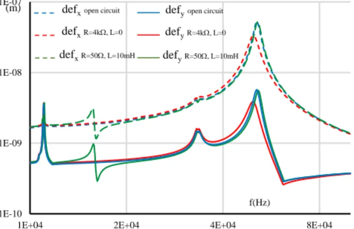
Figure
Documents relatifs
Dans le cadre du présent rapport, cinq sites universitaires ont été retenus comme études de cas : l’université de Bourgogne Dijon-Montmuzard, l’université de Lyon II « Berges
Parmi les théories que Ross considère utiliser le concept de validité dans ce second sens figure la Théorie pure du droit, dans la mesure où la validité de l’ordre juridique y
from Africa (Cameroon, Central African Republic, Ethiopia, Mauritania, Sudan and Togo), 361 from Central and South America (Mexico, Honduras, Venezuela, Peru and French Gui- ana),
Tectonic expression of an active slab tear from high-resolution seismic and bathymetric data offshore Sicily (Ionian Sea). Intra-Messinian truncation surface in the Levant
En revanche, le code de calcul numérique TEHD, lorsque la garniture mécanique est alimentée en eau et qu’il se produit du changement de phase dans l’interface, prédit
L’archive ouverte pluridisciplinaire HAL, est destinée au dépôt et à la diffusion de documents scientifiques de niveau recherche, publiés ou non, émanant des
یئاطع ءهدنشخب هک یمیرک یا یئاطخ ءهدنشوپ هک یمیکح یا و یئادج قلخ کاردا زا هک یدمص یا و یئاتمه یب تافص و تاذ رد هک یدحا یا و یئامنهار هک یقلاخ یا و یئازس ار ییادخ هک
7.1.6. Cauchy surface two-point functions.. Reduction to the model case. We use the notation in Subsect. Without loss of generality we may assume that χ = Id.. The proof is
