A Simple Model for Hardness and Residual Stress Profiles Prediction for Low-Alloy Nitrided Steel, Based on Nitriding-Induced Tempering Effects

A simple model for hardness and residual stress

profiles prediction for low-alloy nitrided steel,

based on nitriding-induced tempering effects

Grégory MICHEL 3

1 _{Safran Tech, Magny les Hameaux – France, simon.thibault@safrangroup.com} 2 NTN-SNR, Annecy – France, christine.sidoroff@ntn-snr.com

3 _{IRT-M2P, Metz – France, gregory.michel@irt-m2p.fr}

4 _{MSMP Laboratory, Arts et Métiers ParisTech, Aix-en-Provence – France, sebastien.jegou@ensam.eu} Abstract

Nitriding of low-alloy steels is widely used for gears and bearings in aerospace industry. Some highly stressed surfaces require high nitrided depth, which involves long time/high temperature nitriding treatment. This study focused on identifying process parameter effects on hardness and residual stress profiles in a large range of nitriding time and temperature. We demonstrate that core and case can be considered as two materials, softening of which can be predicted by two tempering laws. In addition, a basic relationship was derived from the nitriding depth and a pseudo-diffusion coefficient, allowing prediction of the hardness profile. Residual stress results show that the diffusion controlled effect can also be used to predict residual stress profile affected depth. Likewise, the tempering controlled effect can be used to predict surface and maximum values of the residual stress profile.

Keywords

Nitriding, modelling, hardening, tempering, residual stress

1 Introduction

The aerospace industry is continuously looking for weight reduction. Thus, reducing design margins between applied stress and materials strength becomes necessary. In the case of gears and bearings, this can be achieved by mastering surface engineering, especially through thermochemical heat treatments. Recent developments of mechanical design methods at a mesoscopic scale, allow to check if the local mechanical properties are able to undergo a given applied stress field ([Walvekar, 2017], [Savaria, 2015], [Weil, 2018], [Ghribi, 2016], [Hassani-Gangaraj, 2014]). These methods, generally based on the concept of local mechanical limit [Spies, 1993], use hardness profile as strength indicator and residual stress profile as a part of the global stress field. On this basis, a process modelling able to provide both profiles for given process parameters, can be of interest. It can be used to specify process parameters for a given part, or to identify the influence of desired or undesired process parameter changes on mechanical performance.

In the specific case of low-alloy steel nitriding, such models are reported in literature. They are based on combined diffusion and precipitation complex calculations ([Jung, 2015], [Barrallier, 1992], [Jegou, 2016]). Micro-macro mechanical models are then employed to compute residual stress resulting from local differential density of the metallurgical phases formed during nitriding. Nitrogen profile calculations are also used for hardness prediction. Empirical formulations can be found between hardness and nitrogen concentration [Hiraoka, 2016]. They are not suitable for long time or high temperature nitriding required by some highly stressed parts. In fact, they do not take into account decrease of core and case hardness and the important

profile shape change induced by such treatments. More recently, a similar model was proposed to take into account the temperature effect on type and morphology of nitrides, which affect differently local hardness [Weil, 2018]. Finally, we can mention a method linking residual stress profiles to hardness profile [Leskovsek, 2008]. It obviously requires experiments to get the hardness profiles.

The aim of the present work is to propose a tool for engineer for an easy estimation of hardness and residual stress profiles from process parameters, without complex thermodynamics and mechanical calculation steps.

2 Experimental procedure

Coupons of 45 mm in diameter and 12 mm height were cut from a 80 mm diameter bar of normalized and annealed E33CrMoV12-9 steel grade. Then, the samples were quenched (austenitized at 920 °C, quenched in oil at 50 °C) and air tempered (2 hours at 615 °C) to achieve an ultimate tensile stress of around 1300 MPa and 410 HV10 hardness. Surfaces were then ground for a surface finish of 0,4 µm arithmetic roughness.

Nitriding treatments were performed in an ALD industrial nitriding furnace with a large range of nitriding times and temperatures (from 4 to 200 hours and from 480 to 590 °C). The atmosphere control during nitriding was ensured by a H2SMART™ system (UPC). Regulation of the

nitriding potential KN was made by adjusting ammoniac (NH3) and dissociated ammoniac (N2 +

H2) flow rates. All nitriding experiments were done with a KN leading to a continuous compound

layer formation in the temperature range explored (i.e. KN > 0.5 atm-0,5). Thus, the chemical

boundary condition for the diffusion layer is controlled by the maximal nitrogen weight fractioncontent one can introduce in the steel (sum of nitrogen fractioncontent in solid solution, alloying element nitrides and excess nitrogen [Somers, 1989]) which only depends on steel composition and temperature.

Microstructure in cross section was observed by optical microscopy after Nital and Murakami etching. Cross section hardness profiles were obtained with a Qness Q60+ micro hardness testing machine using Vickers indentor and a 0.5 kgf force. For each sample, three hardness profiles were measured. A mean hardness profile was then calculated. Residual stress profile assessment was carried out by X-ray diffraction with a Elphyse SetX device using Cr-Kα radiation on the {211} diffracting plane of α-Fe. The sin2_{ψ method was used to determine the mean residual}

stresses in α-Fe ( S1{211}=−1.25 . 10−6 MPa-1,

1 2S2

{211 }

=5.85 .10−6 MPa-1_{) along the}

nitriding depth. Electro-chemical surface layer removal was performed for in-depth profiling. Nitrogen and carbon weight fractioncontent profiles were obtained thanks to Wavelength Dispersion Spectroscopy (WDS) using Cameca SX100 electron probe micro analyser. As for hardness profiles, three measurements were performed and a mean curve was calculated.

3 Results

Typical results are given in Figure 2 and Figure 3 for a nitriding treatment of 120 hours at 550°C. Optical microscopy observations for both etching are presented in Figure 1. The Nital etching reveals a fine tempered martensitic structure and a homogeneous compound layer (ε + ’). The Murakami etching reveals intergranular cementite precipitation, also called “seagulls”. This is due to carbon migration which results from substitution of originals carbides to globular nitrides.

Figure 1: Typical microstructure of nitrided E33CrMoV12-9 after Murakami (left) and Nital (right) etching.

WDS measurements shows that nitrogen is present in the first 0,8 mm. The sharp gradient from 0,6 to 0,8 mm is due to the precipitation front of MN, where M can be Cr, Mo or V (mainly Cr) [Ginter, 2006]. The carbon fraction content baseline modification (%wt C = 0.32 initially) can be linked with two phenomena: decarburizing during the first steps of nitriding, and substitution of carbides by nitrides [Jegou, 2018]. For this nitriding treatment, surface hardness is 740 HV. Core hardness suffered a slight softening to reach 370 HV. The residual stress profile shows the typical form reported in literature, with a an affected depth higher than the hardness one, and a maximum compressive stress of -400 MPa in the diffusion layer.

Figure 2: WDS nitrogen and carbon weight fractioncontent profile for the 120 hours – 550 °C nitriding experiment

Figure 3: Hardness (left) and residual stress (right) profiles for the 120 hours – 550 °C nitriding experiment and relevant indicators

Values of interest, displayed on Figure 3, were collected for all nitriding experiments. These indicators will be designated in the following sections as detailed in Table 1.

Hardnes s indicator Definition ↗ T° ↗ t Residual stress indicator Definition ↗ T ↗ t

peak(extremum)

HVS _{Surface hardness}1 _{↘↘ ↘ }S _{Surface residual stress} ↘

↘ ↘

NHD* Modified nitriding hardness depth

(HV Core + 20) ↗ ↗↗ z(

P₎ Maximum residual

stress depth ↗ ↗↗

NHD Nitriding hardness depth

(HV Core + 100) ↗ ↗↗ z( -100₎ Residual stress affected depth (Depth at which residual stresses decrease back to-100

MPa)

↗ ↗↗

1

Note that “surface hardness” does not strictly result from a surface measurement but refers to the first cross-section reading of microhardness

Table 1: Indicator definition and their evolution for an increase in nitriding time or temperature. (↗ means

moderate increase - ↘ means moderate decrease - ↘↘ or ↗↗ mean important decrease or increase - =

means no change - parenthesis indicate change occurring for particularly high nitriding duration or time) Since they follow the classical and widely reported trends ([Spies, 2014][ASM, 1991][Ginter, 2006]), the effect of nitriding time and temperature on hardness, residual stress and case depth are given in a simple way in Table 1 but not detailed. Increasing temperature or time resulted in an increase of case depth and in a decrease of case hardness and compressive residual stress. Long time and high temperature treatments can result in a decrease of core hardness [Hoja, 2015].

As Ginter [Ginter, 2006] did in previous works, local hardness was plotted as a function of nitrogen content for various nitriding experiments, leading to different hardening laws. Two representations are proposed in Figure 4. The first one shows hardening laws at the surface for different nitriding durations at 550 °C. The second one shows hardening laws for 120 hours nitriding at different temperatures. One can see that neither temperature nor duration of nitriding treatment is sufficient to describe a hardening law, which seems to obey to a combined time-temperature effect.

Figure 4: Surface hardening laws for nitriding performed at same temperature but different time (left) and for nitriding performed at different temperature but for a given time (right)

4 Model formulation

To depict the combined time/temperature effect mentioned above, and as did Hoja [Hoja, 2015] for core hardness, we propose to link case and core hardness but also residual stress to the well-known Hollomon-Jaffe [Hollomon, 1945] tempering parameter, which allows time/temperature equivalences. Since this parameter was initially used for tempering treatment, we will call it

HPNIT to explicit that, in our case, it represents the intensity of nitriding-induced tempering. As in

the original formulation, HPNIT is calculated thanks to Eq. [1].

HP_NIT=(T + 273.15)(C+ log10(t ))

1000 [1]

Where T is the nitriding temperature in Celsius degrees, t is the nitriding time in hours, and C is a material parameter, generally set to 20 for martensitic steels.

As for martensitic steel tempering, the higher the HP, the lower the hardness. Final surface hardness and residual stresses after nitriding can be considered as the consequence of tempering of freshly nitrogen saturated steel. We assume that, once surface composition is stabilized (few hours [Fallot, 2015][Jegou, 2018]), nitriding acts as a simple tempering treatment on the diffusion layer, leading to phase transformations in terms of size and volume of nitrides and grain boundaries carbides (cementite) [Locquet, 1997],[Barrallier, 2014].

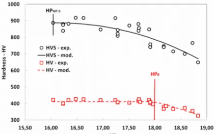
Four points of interest are needed to draw the calculated hardness profile. The first ones are the surface and core hardness values, respectively named HVS _{and HV. Figure 5 represents}

experimental values of HVS _{and HV versus HP}

NIT. A good correlation can be found between

surface hardness decrease and HPNIT, whatever the nitriding temperatures and times considered.

For core hardness, a transition is observed when HPNIT reaches the critical HP value

corresponding to the initial tempering treatment. We call this parameter, the Hollomon-Jaffe reference parameter for core steel, HP0 (in our case, HP0 = 18). If HPNIT exceeds HP0, core

Figure 5: Surface hardness HVS _{and core hardness HV as a function of HP}

NIT parameter

Thus, the following functions (equations [2, 3]) can be used to predict HVS _{and HV as a function}

of HPNIT:

HV =H V₀−¿HP_NIT−H P₀>[2]

HVS

=HV₀S−❑S

₍

₎

Where HV0 is the core hardness before nitriding. HVS0 is the reference surface hardness

corresponding to the surface hardness reached for the lowest value of HPNIT nitriding experiment,

called HPNIT0. , S and n are dimensionless model parameters. < > are the Mac Cauley brackets.

Nitriding hardness depth NHD, in mm, can be related to nitriding time t and temperature T through a simplified diffusion calculation described in Eq. [4].

NHD=1000

√

ED

8.314 (T+273.15)_{.3600 .t [4 ]}

Where D0 is a pseudo-diffusion coefficient in µm2s-1 and ED is the activation energy in J.mol-1.

Comparison between experimental data and calculation of NHD is given in Figure 6.

To complete the hardness profile, a modified NHD, called NHD* was defined (see Figure 3). Figure 7 shows that this indicator can be directly linked to NHD with a linear relation defined in Eq. [5].

NHD¿

Figure 6 : Nitriding hardness depth NHD as a function of nitriding time t for three nitriding

temperature T

Figure 7: Modified nitriding hardness depth NHD* as a function of NHD

HPNIT was also successfully used to describe the evolution of residual stress values at the surface

(S) and at the peak (P_{) as a function of nitriding parameters (see Figure 8). Both values can be}

calculated with the type of function previously used for hardness (Eq. [6, 7]).

❑S=−❑₀S+❑S

₍

₎

❑P=−❑₀S+❑P

₍

₎

Where S

0 is the reference surface residual stress corresponding to the surface residual stress

reached for the lowest value of HPNIT nitriding experiments called HPNIT0. S, P and m are

dimensionless model parameters.

Finally, maximum residual stress depth (z(P₎) and residual stress affected depth (_z(-100₎) are

derived from NHD calculated values with linear relations given in Eq. [8, 9] (see Figure 8 and Figure 9).

z (❑P)=. NHD [8] z (❑−100)=. z (❑P)[9 ]

Figure 8: Surface S _{and peak }S _{residual stress}

versus nitriding parameter HPNIT

All parameters needed for the model, their way of identification and the mean deviation between calculated and experimental values for all nitriding experiments are summarized in Table 2.

Paramete

r Identification

Mean

deviation Parameter Identification Mean deviation

C [Hollomon, 1945] - D0 NHD = f(t,T) best fit 9 % (0,02 mm) HP0 Tempering steel conditions (T, t) -ED HV0  NHD*=f(NHD) best fit 13 % (0,05 mm) HPNIT0 Lowest HPNIT experiment -m S _{and }P _{= f(HP} NIT) best fit 18 and 5 % (45 and 24 MPa) HV0S S 0S P S HVS _{= f(HP} NIT) best fit 4 % (32 HV)  z(P) = f(NHD) best fit 38 % /(1)_{11 %} (0,049 /(1)_{0,04 mm)}

n (1) calculated deviation without nitriding experimentsperformed at 480 °C, for which peak stress position is difficult to identify experimentally

 HV = f(HPNIT)

best fit 2 % (10 HV)  z(

-100_{) = f(z(}P_{)) best fit 13 % (0,1 mm)}

Table 2: Model parameters, their way of identification, and mean deviation between calculated and experimental value for the whole nitriding experiments

Parameters values leading to best fits were obtained by minimizing the error function defined in [10] with the Excel® solver.

error function=

_∑

(I_exp−I_mod)2[10]

Where x is the number of experiments performed, Iexp and Imod are respectively the experimental

and modelled indicator values.

Figure 10 gives a comparison between experimental and calculated profiles for three nitriding conditions, covering a large range of HPNIT values, 16.04, 17.51 and 18.83 (respectively

480°C/20 h, 550°C/120 h and 580°C/120 h). It is important to remember that shape of hardness profile between surface hardness and NHD is not described since the assumption of the model is only suitable for surface and core.

Figure 10: Model versus experiment for three nitriding conditions: hardness profile (left) and residual stress profile (right)

These experiments correspond to three tempering regimes (see Figure 5). For the lowest value of

HPNIT, case and core hardness are maximum and not yet affected by tempering effect. For the

intermediate one, surface softening has begun whereas core hardness is not affected. For the higher one, both surface and core are softened because of nitriding-induced tempering. These different regimes are well described by our model. Residual stress profiles prediction is also convenient.

5 Model validation

In order to validate the proposed model, three new nitriding experiments, detailed in Table 3, were done with the same HPNIT values but different values of t and T. First of all, it can be seen

in Figure 11 that nitriding treatments performed with the same HPNIT parameter lead to almost

the same hardening laws. Previous nitriding results with close HPNIT value are also plotted to

confirm our fundamental model assumption.

Experiment t (h) T (°C) HPNIT

#1 200 520 17,69

#2 106 530 17,69

#3 58 540 17,69

Figure 11: Hardening laws for nitriding experiments with close HPNIT values

A comparison is given in Figure 12 between experimental and calculated profiles for the three iso-HPNIT treatments.

Figure 12: Model versus experiment for the three validation nitriding experiments. Hardness profiles (left) and residual stress profiles (right)

These results confirm globally the fact that a given HPNIT induces given surface and core

hardness but also surface and maximum residual stress. A quite good estimation of both profiles is obtained with the model.

6 Conclusion

By scanning a large range of nitriding time and temperature, we demonstrated that hardness and residual stress profiles can be easily estimated by considering nitriding-induced tempering effects and basic diffusion calculation. This calculation can be performed thanks to a simple engineering parameter, HPNIT. This parameter combines nitriding temperature and time effects on hardness

and residual stress values. The relevance of this process parameter was demonstrated experimentally thanks to iso-HPNIT nitriding experiments. The model is presented in Figure 13 in

an abacus shape. Nitriding conditions can be quickly identified from specified NHD, hardness and residual stress values.

Figure 13: Abacus for NHD (isothermal and isochronous black curves), HVS_{, HV (red curves), -}P _and

z(P_{) (green curves) estimation from nitriding time and temperature traduced in terms of HP}

NIT for

E33CrMov12-9 steel. An example of solutions complying requirements is given in blue.

Even though there is a unique nitriding solution for a determined specification, various nitriding solutions can be found for a range of targeted values. An example is given in Figure 13. The given specification (see top of Figure 13) can be achieved with a large range of nitriding duration (from about 60 h to 140 h). In this case, nitriding temperature limitation comes from the core requirement. The resulting residual stress peak should vary between roughly -450 and -500 MPa. Theoretically, the model parameters can be identified for another low-alloy nitriding steel or other pre-treatment, with only three experiments (including nitriding, hardness testing and residual stress measurement). Nevertheless, five experiments, uniformly distributed in the 16-19

HPNIT range are recommended.

Acknowledgements

This work was supported by the French government PIA (Programme d’Investissements d’Avenir) through the IRT-M2P “NITRU” project. The authors deeply thank the other industrial partners (mentioned in alphabetic order):

Airbus Group, Air-Liquide, ALD, Naval Group, Sofiplast, UTC Ratier-Figeac. The authors also thank Q. MILLEE (IRT-M2P) for nitriding treatments and characterizations.

References

ASM Hanbook, Gas nitriding of steel, in Heat Treating, ASM International, vol. 4, 1991

L. Barrallier, Genèse des contraintes résiduelles de nitruration – Etude expérimentale et modélisation. PhD thesis, ENSAM, Aix-en-Provence,1992

L. Barrallier, Classical nitriding of heat treatable steel, Thermochemical Surface Engineering of Steels. Woodhead Publishing. 2014, 392-411

G. Fallot, Rôle du carbone lors de la nitruration d’aciers de construction et influence sur les propriétés mécaniques. PhD thesis, ENSAM, Aix-en-Provence, 2015

D. Ghribi, M. Octrue, P. Sainsot. Etude des ruptures internes des flancs des dentures, tooth flank fracture, Journées Transmissions Mécaniques, Lyon, 2016

C. Ginter, Influence des éléments d’addition sur l’enrichissement d’azote et le durcissement d’aciers nitrurés. PhD thesis, Université de Nancy, 2006

S.M. Hassani-Gangaraj, Moridi et al., The effect of nitriding, severe shot peening and their combination on the fatigue behavior and micro-structure of a low-alloy steel, International Journal of Fatigue 62, 2014, 67–76

Y. Hiraoka,Y. Watanabe, O. Umezawa, Practical model to predict diffusion layer’s hardness profile in gas nitrided low alloy steel containing chromium. J.Japan Inst. Met.Mater.,vol. 80, 2016, 259–267

S. Hoja, Hoffman et al., Design of deep nitriding treatment for gears, Journal of Heat Treatment of materials, vol. 70, 2015

Hollomon, Jaffe, Time-temperature relations in tempering steel, Trans. AIME, 1945

S. Jégou, L. Barrallier, G. Fallot, Optimization of gaseous nitriding of steels by multi-physics modelling. 23rd International Federation of Heat Treatment and Surface Engineering Congress 2016, 63–70, 2016

S. Jégou, L. Barrallier, G. Fallot, Gaseous nitriding behavior of 33CrMoV12-9 steel: Evolution of the grain boundaries precipitation and influence on residual stress development, Surface &Coating Technology 339 (2018) 78-90

M. Jung, Meka, et al., Coupling Inward Diffusion and Precipitation Kinetics; the Case of Nitriding Iron-Based Alloys, Metallurgical and Material Transactions A, vol. 47A, 2016

V. Leskovšeka, B. Podgornikb, D. Nolanc, Modelling of residual stress profiles in plasma nitride tool steel. Material Characterization, vol. 59, 2008, 454-461

J.N. Locquet, Caractérisations métallurgiques et mécaniques de couches nitrurées, relation microstructure comportement. PhD thesis, ENSAMd’Aix-en-Provence,1998

V. Savaria, F. Bridier, P. Bocher, Predicting the effects of material properties gradient and residual stresses on the bending fatigue strength of induction hardened aeronautical gears, International Journal of Fatigue, vol. 85, 2016, 70-84

M.A.J. Somers, R.M. Lankreijer, E.J. Mittemeijer, Excess nitrogen in ferrite matrix of nitrided binary iron-bases alloys. Philosophical Magazine A, vol. 59, 1989, 353-378

H.J. Spies, Fatigue behaviour of nitrided steels, Steel Research, 1993

H.J. Spies, Case Structure and Properties of Nitrided Steels, Comprehensive Materials Processing, vol. 12, Elsevier, 2014

A.A. Walvekar, F. Sadeghi, Rolling Contact Fatigue of Case Carburized Steels, International Journal of Fatigue, vol. 95, 2017, 264-281

H. Weil, L. Barrallier, S. Jegou, N. Caldeira-Meulnotte, G. Beck, Optimization of gaseous nitriding of carbon iron-based alloy iron-based on fatigue resistance modelling, International Journal of Fatigue, vol. 110, 2018, 238–245