UNIVERSITÉ DE MONTRÉAL
MODEL PREDICTIVE CONTROL OF BUILDING SYSTEMS FOR ENERGY FLEXIBILITY
KUN ZHANG
DÉPARTEMENT DE GÉNIE MÉCANIQUE ÉCOLE POLYTECHNIQUE DE MONTRÉAL
THÈSE PRÉSENTÉE EN VUE DE L’OBTENTION DU DIPLÔME DE PHILOSOPHIAE DOCTOR (Ph. D.)
(GÉNIE MÉCANIQUE) OCTOBRE 2018
UNIVERSITÉ DE MONTRÉAL
ÉCOLE POLYTECHNIQUE DE MONTRÉAL
Cette thèse intitulée :
MODEL PREDICTIVE CONTROL OF BUILDING SYSTEMS FOR ENERGY FLEXIBILITY
présentée par : ZHANG Kun
en vue de l’obtention du diplôme de : Philosophiae Doctor a été dûment acceptée par le jury d’examen constitué de :
M. CIMMINO Massimo, Ph. D., président
M. KUMMERT Michaël, Ph. D., membre et directeur de recherche M. ANJOS Miguel F., Ph. D., membre
ACKNOWLEDGEMENTS
My greatest thanks go to my supervisor Prof. Michaël Kummert. I am really grateful for your guidance, support, suggestions and invaluable time throughout the different projects in my graduate studies. Thank you for your confidence to let me work within the IEA Annex 67 project and present my work at different conferences and meetings across the world. Those opportunities have broadened my horizons in the research field. Your encouragement, positive feedback and kind personality have made this journey enjoyable.
I wish to extend my gratitude to Prof. Michel Bernier. Thank you for your valuable advice on my work and for giving me the opportunities to work as your teaching assistant through those years. I am also appreciative to Dr. Massimo Cimmino for his recommendation for my future career. The casual talks we had in and outside the office were delightful.
I would like to thank the past and present members of the Bee(r) Lab: Katherine D'Avignon, Benoit Delcroix, Humberto Quintana, Samuel Letellier-Duchesne, Behzad B. Bafrouei, Camille Beurcq, Alex Laferrière, Louis Leroy, Walid Lallam, Adam Neale, Houaida Saidi. Thank you for your help on the technical and nontechnical issues I have encountered. You made the lab life and the time away from home more pleasant.
I also acknowledge the following entities for their funding support: NSERC, SNEBRN, Sumaran, and Stelpro. I could not carry out this research without their generous contributions.
At last, a special thank you to my family and friends for your love and always being there, actually or virtually.
RÉSUMÉ
Les besoins énergétiques des bâtiments contribuent de manière significative à la demande de pointe du réseau électrique. Cependant, les bâtiments, par leur capacité de stockage de l’énergie, peuvent fournir des services de flexibilité énergétique au réseau. La Gestion de la Demande de Puissance (GDP) du bâtiment est considérée comme une solution pratique pour réduire les demandes de pointe du réseau. Cette approche est moins coûteuse et plus écologique que d’utiliser la réserve de puissance ou que d'investir dans de nouvelles infrastructures. La GDP peut également jouer un rôle plus important au niveau de l’équilibrage de charge, lorsque le réseau intègre des sources d’énergie renouvelables, qui sont intermittentes et variables.
Cette thèse étudie le potentiel de flexibilité énergétique des bâtiments vis-à-vis du réseau électrique par le biais de la simulation. Une méthodologie générale pour caractériser la flexibilité énergétique des bâtiments, ainsi qu’un ensemble d’indicateurs sont proposés. La méthodologie est testée sur un modèle détaillé de maison canadienne type, calibré avec des données mensuelles et horaires mesurées. La calibration permet de représenter fidèlement la consommation d'énergie selon les critères de la directive 14 de l’ASHRAE, ainsi que les variations dynamiques des conditions thermiques intérieures, ce qui est nécessaire pour l'étude des stratégies de commande. Les résultats des simulations, basés sur ce modèle calibré, montrent que la flexibilité énergétique fournie par la masse thermique du bâtiment est importante, même pour les bâtiments résidentiels à faible masse thermique. La quantité d'énergie flexible dépend cependant des conditions météorologiques, de l'heure du jour, de la durée de la GDP et de l'occupation du bâtiment.
La flexibilité énergétique est également fortement liée à la stratégie de commande du système de chauffage et climatisation. Une méthode de contrôle avancée est étudiée : la Commande Prédictive basée sur un Modèle (CPM). Avant d’appliquer cette méthode à la flexibilité énergétique, un cadre général de CPM est proposé. Les erreurs de modélisation, l’estimation de l’état et l’identification des paramètres y sont discutées en détail. Ce cadre est ensuite appliqué à deux types de modèles de contrôleurs différents : un modèle détaillé et un modèle simplifié du bâtiment étudié.
Les résultats montrent que la CPM peut améliorer la flexibilité énergétique par rapport à une stratégie de Commande Basée sur les Règles (CBR). La flexibilité énergétique obtenue par une
CPM avec modèle détaillé est la plus élevée. Cette énergie est deux à trois fois supérieure à celle obtenue par une stratégie CBR, selon l'heure de l'évènement de la GDP. L'énergie flexible obtenue par une MPC avec modèle simplifié est moindre que celle avec modèle détaillé. Mais son coût de calcul est beaucoup moins cher. Il est similaire à celui de la méthode CBR : de l’ordre de quelques secondes. D’autre part, l'effet de rebond des méthodes CPM est plus prononcé, ce qui génère une efficacité flexible inférieure à celle de la stratégie CBR.
ABSTRACT
Energy needs from buildings contribute a large share to the peak demand of the electric grid. Meanwhile, buildings can also provide energy flexibility services to the grid with their related assets, e.g. energy storage. Demand Response (DR) of building systems has been considered a feasible solution to shift loads, or to reduce the peak demands. This approach is less costly and more environmentally-friendly than operating reserve power, or investing in extra power plants. DR can play a more important role for load balancing when the grid integrates with renewable energy sources, which are intermittent and variable.
This thesis investigates the energy flexibility potential in buildings for the grid through simulation studies. A general methodology to characterize the building energy flexibility is proposed along with a set of indicators. The methodology is applied to a detailed building model of a typical Canadian home, which is calibrated with monthly and hourly measured data. The calibration evaluates not only the energy use required by the ASHRAE guideline 14, but also the dynamic indoor conditions, which is important to study control strategies.
Simulation results, based on the calibrated model, show that the energy flexibility provided by the building thermal mass is significant, even for typical Canadian residential buildings with a low thermal mass. The amount of flexible energy however depends on the weather condition, time of day, duration of the DR event and occupancy scenario of the building.
The control strategy of the space conditioning system has also a high impact on the energy flexibility. An advanced control method called Model Predictive Control (MPC) is investigated. Prior to applying the MPC method on energy flexibility study, a general supervisory MPC framework is presented. Common issues associated with modelling errors, state estimation, and parameter identification are discussed in detail. The framework is then applied to two different types of controller models: a detailed model and a simplified model of the studied building respectively.
The MPC method is shown to be able to increase the building flexibility as compared to the Rule-Based Control (RBC) strategy. MPC with the detailed model delivers the highest flexible energy, twice or three times of the RBC method depending on the time of the DR event. MPC with the simplified model presents less flexible energy than that with the detailed model, but its
computation cost is also less expensive, in the same magnitude as the RBC method in seconds. On the other hand, the rebound effect of the MPC methods is more pronounced, resulting in lower flexible efficiency than RBC.
TABLE OF CONTENTS
ACKNOWLEDGEMENTS ... III RÉSUMÉ ... IV ABSTRACT ... VI TABLE OF CONTENTS ... VIII LIST OF TABLES ... XI LIST OF FIGURES ... XII LIST OF SYMBOLS AND ABBREVIATIONS... XV LIST OF APPENDICES ... XX CHAPTER 1 INTRODUCTION ... 1 1.1 Context ... 1 1.2 Objectives ... 4 1.3 Structure ... 5 1.4 Contributions ... 6
CHAPTER 2 DETAILED BUILDING MODEL... 8
2.1 Introduction ... 8
2.2 Methodology ... 15
2.3 Detailed modelling in TRNSYS ... 17
2.4 Calibration results ... 23
2.5 Discussions ... 36
CHAPTER 3 ENERGY FLEXIBILITY CHARACTERIZATION ... 38
3.1 Introduction ... 38
3.2 Methodology ... 40
3.4 Sensitivity analysis ... 45
3.5 Discussions ... 54
CHAPTER 4 MODEL PREDICTIVE CONTROL FRAMEWORK ... 56
4.1 Introduction ... 56
4.2 Methodology ... 60
4.3 MPC without model mismatch ... 63
4.4 MPC with online parameter identification ... 69
4.5 MPC with state estimation ... 73
4.6 Discussions ... 75
CHAPTER 5 MODEL PREDICTIVE CONTROL WITH DETAILED MODEL ... 77
5.1 Introduction ... 77
5.2 Methodology ... 79
5.3 Results of a single DR event ... 82
5.4 Results with occupancy constraint ... 84
5.5 Discussions ... 95
CHAPTER 6 MODEL PREDICTIVE CONTROL WITH SIMPLIFIED MODEL ... 96
6.1 Introduction ... 96
6.2 Methodology ... 100
6.3 MPC results ... 104
6.4 Sensitivity analysis ... 106
6.5 Comparison between MPC and RBC ... 108
6.6 Discussions ... 109
CHAPTER 7 CONCLUSION AND RECOMMENDATIONS ... 111
7.2 Conclusions ... 112
7.3 Further studies ... 113
BIBLIOGRAPHY ... 114
LIST OF TABLES
Table 2.1: Brief characteristics of CCHT houses ... 11
Table 2.2: Summary of available measurements ... 12
Table 2.3: Criteria of calibrated building energy models ... 16
Table 2.4: Type 1244 (3D ground coupling) parameters ... 20
Table 2.5: Annual energy use, measured and simulated ... 24
Table 2.6: ASHRAE goodness-of-fit indicators for daily energy use ... 28
Table 2.7: ASHRAE goodness-of-fit indicators for hourly energy use ... 29
Table 2.8: Model sensitivity to key parameters ... 34
Table 3.1: Reference setpoint scenario ... 43
Table 3.2: Reference setback profile ... 53
Table 5.1: Flexibility results of MPC for a single DR event (downward flexibility) ... 83
Table 5.2: Flexibility results of MPC for two consecutive DR events ... 86
Table 5.3: Power demand reduction and computation time ... 92
Table 5.4: Summary of flexible results of MPC and heuristic approaches (morning peak) ... 93
Table 5.5: Summary of flexible results of MPC and heuristic approaches (afternoon peak) ... 93
LIST OF FIGURES
Figure 1.1: IESO daily power demand ... 1
Figure 1.2: Hydro-Quebec seasonal critical peak demand ... 2
Figure 1.3: Structure of the thesis ... 5
Figure 2.1: Canadian Centre for Housing Technology (CCHT) twin houses ... 11
Figure 2.2: Daily average ambient temperature - weather data file vs. measured values ... 13
Figure 2.3: Global horizontal solar radiation - weather data file vs. measured values ... 13
Figure 2.4: Global horizontal solar radiation - weather data file vs. measured values (August) ... 14
Figure 2.5: Global horizontal solar radiation - weather data file vs. measured values (March) .... 15
Figure 2.6: Floor plans of the CCHT houses ... 18
Figure 2.7: The first layer of the 3D ground model input file ... 19
Figure 2.8: Diagram of a forced air system with HRV ... 21
Figure 2.9: Monthly furnace gas and air-conditioner electricity use ... 25
Figure 2.10: Daily furnace gas and air-conditioner electricity use ... 27
Figure 2.11: Daily error on furnace gas and air-conditioner electricity use ... 27
Figure 2.12: Room temperatures - hourly measured and simulated values ... 28
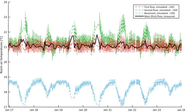
Figure 2.13: Hourly measured main floor temperature and simulated 5-min values – winter ... 30
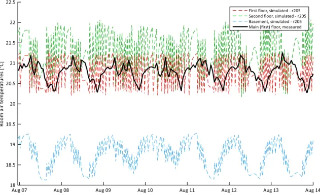
Figure 2.14: Hourly measured main floor temperature and simulated 5-min values – summer .... 31
Figure 2.15: Furnace gas input and main floor temperature Jan 21 and 22 ... 32
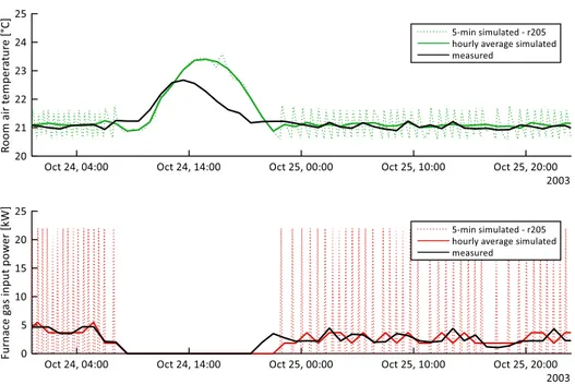
Figure 2.16: Furnace gas input and main floor temperature for October 24 and 25 ... 32
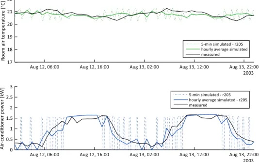
Figure 2.17: Air-conditioner power use - August 12 and 13 ... 33
Figure 2.18: Air-conditioner power use - October 8 and 9 ... 33
Figure 3.1: Flexible energy demand of buildings (downward flexibility) ... 41
Figure 3.3: Downward flexible energy of the heating season ... 47
Figure 3.4: Upward flexible energy of the heating season ... 47
Figure 3.5: Downward flexible efficiency of the heating season ... 48
Figure 3.6: Upward flexible efficiency of the heating season ... 48
Figure 3.7: Flexible energy as a function of DR duration ... 49
Figure 3.8: Rebound energy as a function of DR duration ... 50
Figure 3.9: Median flexible efficiency as a function of DR duration ... 50
Figure 3.10: Maximum flexible power vs. DR duration ... 51
Figure 3.11: Setpoint temperature change ... 52
Figure 3.12: Setback setpoint scenario ... 53
Figure 4.1: MPC scheme for supervisory control ... 61
Figure 4.2: Sketch of an example 2-zone building ... 62
Figure 4.3: RC network of the lumped-capacitance model ... 64
Figure 4.4: Validation of the controller model in Matlab ... 65
Figure 4.5: MPC results without model mismatch ... 68
Figure 4.6: The predictive temperature at each time step (15 min) ... 69
Figure 4.7: MPC results with parameter estimation (Zone 1) ... 71
Figure 4.8: MPC results with parameter estimation (Zone 2) ... 72
Figure 4.9: MPC results with state estimation (Zone 1) ... 74
Figure 4.10: MPC results with state estimation (Zone 2) ... 75
Figure 5.1: Flexible energy demand of buildings with MPC (downward flexibility)... 79
Figure 5.2: MPC scheme with TRNSYS and GenOpt (Quintana & Kummert, 2015) ... 81
Figure 5.3: MPC results for a downward flexibility event ... 83
Figure 5.5: Heuristic MPC with an optimal Jump setpoint profile ... 88
Figure 5.6: Heuristic MPC with an optimal Linear setpoint profile ... 89
Figure 5.7: Heuristic MPC with an optimal Exponential setpoint profile ... 89
Figure 5.8: Heuristic MPC with Minimum Power at peak time ... 90
Figure 5.9: Night setback profile... 91
Figure 5.10: Brute-force MPC with poor initial values ... 94
Figure 6.1: RC network representation of a building wall using different nodes ... 96
Figure 6.2: Co-simulation in BCVTB with Matlab and EnergyPlus (Ma. et al., 2012) ... 99
Figure 6.3: RC model schematic ... 100
Figure 6.4: Validation results of the RC model ... 103
Figure 6.5: MPC with RC network model ... 105
Figure 6.6: MPC results with state-space model ... 107
LIST OF SYMBOLS AND ABBREVIATIONS
Symbols
𝐴, 𝐵, 𝐶, 𝐷, 𝐾 State-space representation matrices [-] 𝐶 Thermal capacitance [J/kg-K]
𝑒 Error [-]
𝐸 Energy [kWh]
𝑓 Coefficient factor [-] 𝐽 Objective function value 𝑘 Thermal conductivity [W/m-K]
𝑚 Flowrate [kg/h]
𝑁 Number of measurements [-]
𝑃 Power [kW]
𝑄 Heat flow rate [W]
𝑅 Thermal resistance [m2K/W]
𝑡 Time [s]
𝑇 Temperature [°C]
𝑈 Controlled input
𝑈𝑝 Thermal conductance [W/K] 𝑈𝐴 Heat transfer coefficient [W/K]
𝑊 Uncontrolled inputs
𝑥, 𝑋 Inputs
𝑦 Values (simulated or measured)
𝑌 Outputs
Greek symbols
𝛼 Coefficient of solar radiation [-]
𝜌 Density [kg/m3]
𝜀 Effectiveness of heat recovery ventilation system [-] 𝜂 Flexible energy efficiency [-]
Subscripts 𝑎, 𝑎𝑚𝑏 Ambient 𝑏 Basement 𝑐 Continuous 𝑑 Discrete 𝑑𝑟 Demand response 𝑓 Flexible 𝑔 Ground 𝑖𝑔 Internal gains 𝑖𝑛𝑒𝑞 Inequality 𝑖𝑛𝑓 Infiltration ℎ Heating 𝑙 Living room 𝑚 Measurement 𝑚𝑖𝑛 Minimum
𝑚𝑎𝑥 Maximum 𝑝 Prediction 𝑟𝑏 Rebound 𝑟𝑒𝑓 Reference 𝑠 Sleeping room 𝑠𝑎 Supply air 𝑠𝑔 Solar gains Abbreviations ACH AIM ANN ARMA ARMAX ARX ASHRAE BCVTB BPS CBR CCHT COP CPM CVRMSE
Air Changes per Hour Alberta infiltration model Artificial Neural Network Autoregressive Moving Average ARMA with exogenous terms
Autoregressive with Exogenous terms
American Society of Heating, Refrigeration and Air-conditioning Engineers Building Controls Virtual Test Bed
Building Performance Simulation Commande Basée sur les Règles
Canadian Centre for Housing Technology Coefficient of Performance
Commande Prédictive basée sur un Modèle
CWEC DR DHW DSM EBC ECM EPBD FEMP GDP GPS HRV HVAC IEA IESO IoT IPMVP ISO KPI LEED LTE MBE MPC M&V NMBE
Canadian Weather for Energy Calculation Demand Response
Domestic Hot Water Demand Side Management
Energy in Buildings and Communities Energy Conservation Measures
Energy Performance of Building Directive Federal Energy Management Program Gestion de la Demande de Puissance Generalized Pattern Search algorithm Heat Recovery Ventilator
Heating, Ventilation and Air Conditioning International Energy Agency
Independent Electricity System Operator Internet of Things
International Performance Measurement and Verification Protocol Independent System Operator
Key Performance Indicators
Leadership in Energy and Environmental Design Laboratoire des technologies de l’énergie
Mean Bias Error
Model Predictive Control Monitoring and Verification Normalized Mean Bias Error
PID PSO PV RMSE RBC RC RES RR SRI TOU USGBC VAV Proportional-Integral-Derivative Particle Swarm Optimization Photovoltaic
Root Mean Squared Error Rule-Based Control
Resistance and Capacitance Renewable Energy Sources Reset Ratio
Smart Readiness Indicator Time of Use
United States Green Building Council Variable Air Volume
LIST OF APPENDICES
Appendix A ... 125
A.1 State equation solutions ... 125
A.2 Predictive output formulation ... 125
CHAPTER 1
INTRODUCTION
1.1 Context
The electric grid generally experiences on-peak and off-peak times on a daily basis, which are highly correlated with human activities. The blue curve in Figure 1.1 shows the power demand of Ontario’s utility Independent Electricity System Operator (IESO) in four consecutive days from December 27 to December 30, 2017, where two peaks can be observed each day in this winter month (IESO, 2016). This shape of daily demand profile with a morning peak, an afternoon dip, and another evening peak is very typical. When a large amount of generation from photovoltaic (PV) panels adds to the grid on a sunny day, the system curve displays an even more obvious “belly” appearance in the midday and a steep rise after the sunset, portraying the silhouette of a duck. This phenomenon of grid demand profile is also known as “duck curve” (Denholm, O’Connell, Brinkman, & Jorgenson, 2015).
Figure 1.1: IESO daily power demand
The grid also experiences seasonal critical peak periods, i.e. the annual highest peak demand hours. For instance, the critical peak hours for IESO annually occur in summer due to air conditioning loads; while for Hydro-Quebec, the utility company in Quebec, the critical peak hours happen in winter because of space heating demands. Figure 1.2 shows the annual critical
peak durations on January 17 in the year of 2009 for Hydro-Quebec. It can be seen that the highest peak demand occurred in the morning at around 7 AM.
Figure 1.2: Hydro-Quebec seasonal critical peak demand
The grid has traditionally been regulated to control the supply to meet demand variations, where grid reliability or resilience requires balancing demand and supply. Historically, the balancing has been technically achieved from the supply side: operating reserve generators when there is supply shortage; or curtailing generation during oversupply. The last issue has been a growing occurrence for grids integrated with Renewable Energy Sources (RES), for example, for the Californian utility California Independent System Operator (California ISO, 2017) and also for the German grid (Schwarz & Cai, 2017).
Another approach for flattening the demand curve is through Demand Response (DR), where consumers adjust their electricity usage during a certain amount of time in response to grid signals. The signals can be time-based rates, penalties, contracts or other forms of financial tools. Considering the electricity as a commodity, it can be bought and sold like stocks in spot markets. Energy policy researchers have been studying this topic, which is outside of the scope of this work.
DR has been proven less costly and more environment-friendly than operating reserve power or investing in extra plants when the capacity is insufficient for the peak demand (Davito, Tai, & Uhlaner, 2010). It can play a more significant role for the load balancing when the RES are
integrated to the grid, where the variable generation power and dependence on climate conditions of the renewables add more challenges to the grid balance.
On the consumption side, the power demand of Heating, Ventilation, and Air Conditioning (HVAC) systems in buildings contributes significantly to the grid peak power demand. In Ontario, the summer peak demand is dominated by residential air conditioning with almost 22% of the peak demand (Hydro One, 2003). In Quebec, it is estimated that residential electric heating accounts for 30% of the winter peak, with a market share of 70% (Kummert, Leduc, & Moreau, 2011). Buildings can, therefore, play an important role in DR. The magnitude and flexibility of buildings’ energy demand can actually become a key asset for DR if well managed (Li, Dane, Finck, & Zeiler, 2017).
DR programs have been successfully implemented in practice to shift the peak power demand of buildings from critical periods to off-peak time (Palensky & Dietrich, 2011). For instance, the utility could turn off heat pumps or electric water heating systems in buildings during peak time through direct load control. In Ontario, a DR program in residential HVAC systems has been promoted through voluntary participation. The device installed in homes receives signals from the grid to cycle down the air conditioner during peak hours. The participants benefit by paying less for on-peak electricity. Hydro-Quebec also tested several experimental DR programs with its employees’ homes (Fournier, Leduc, & Sansregret, 2018; Laurencelle & Moreau, 2018).
Besides the “direct control” program discussed above, another “indirect control” approach may be more practical, where buildings can actively respond to grid signals rather than being passively controlled by the grid directly.
With the effort of grid modernization or “smart grid”, demand-response buildings can help facilitate and optimize grid operations, resources, and infrastructure. This possibility of demand response of buildings is provided by the temporal elasticity of building energy demand, or more concretely, the energy flexibility of buildings.
The energy flexibility of a building is defined broadly as “the ability to manage its demand and (energy) generation according to its local climate conditions, user needs and energy network requirements” by the Annex 67 of the International Energy Agency (IEA) Energy in Buildings and Communities Programme (EBC) (Jensen, Marszal-Pomianowska, et al., 2017).
The flexibility of buildings is largely contributed by energy storage systems (e.g. thermal mass, hot water tanks, ice storage, phase change materials, battery) or energy generation systems (e.g. photovoltaic panels, solar thermal collectors, wind turbines) in or around buildings, or fuel switch if more than one type of fuel is available to supply the building energy needs.
This new terminology is closely related to more established terms like load shifting or load shedding, but it is a more general concept and can be applied to broader circumstances, especially for future smart grid and intelligent buildings, where two-way communications between the grid and buildings would become a common practice. It can act as a label for buildings similar to the energy performance certificate practice carried out in many countries. A position paper published by the Annex 67 more thoroughly explained the context and functionality of energy flexible buildings (Jensen, Henrik, et al., 2017).
A closely related project called “Smart Readiness Indicator (SRI)” for buildings has been launched by the European Energy Performance of Building Directive (EPBD) since 2017, where flexibility is one of the impact criteria for the smartness of buildings. Based on eight different criteria, a single score is given to the assessed building classifying its smart readiness (Vito NV, 2018). The United States Green Building Council (USGBC) and New Building Institute have also initiated a project called GridOptimal in mid-2018. The two institutes aim at creating a rating system with standardized metrics and guidance for building-grid interactions, somewhat similar to the well-established Leadership in Energy and Environmental Design (LEED) program of USGBC (New Buildings Institute, 2018).
In summary, the new operating conditions (e.g. RES integration, oversupply risk) of the electric grid require novel concepts and methodologies to tackle the associated problems. With the advancement of internet and communication technologies, buildings, with its embedded energy flexibility, can contribute significantly to the process of grid modernization, as well as the indispensable part of the smart grid.
1.2 Objectives
The overall goal of the dissertation is to study the potential of building energy flexibility for the grid through simulation studies. It aims at investigating how the advanced control strategy Model Predictive Control (MPC) can contribute to the flexibility potential which is highly impacted by
the HVAC control method. The thesis further aims at proposing a general methodology with simple indicators to quantify the amount of energy flexibility.
More specifically, the objectives of the work can be summarized into the following items:
• Constructing reliable models of the studied building system in order to apply MPC strategy as modelling is the first part of the proposed control approach;
• Proposing a general MPC framework which works for different purposes including energy flexibility;
• Investigating a general method with universal Key Performance Indicators (KPIs) to quantify the energy flexibility including using different control strategies;
• Applying the defined MPC framework for energy flexibility simulation and quantifying the flexibility potential according to the investigated KPIs.
1.3 Structure
Based on the aforementioned objectives, the structure of the thesis is illustrated in the following diagram.
Figure 1.3: Structure of the thesis
Chapter 1 is an overview of the thesis which illustrates the background and objective of the study.
Chapter 2 presents the construction and calibration process for a detailed building model. This simulated building is the basis of the thesis; therefore this chapter is devoted to detailing the modelling and calibrating results. The calibrated model is further used to investigate the general methodology to quantify building energy flexibility and to test the proposed KPIs in Chapter 3. The detailed building model is also employed to identify simplified models in Chapter 5 and used
as the model for MPC in Chapter 6. The arrows in Figure 1.3 visualizes the connections among the chapters.
Based on the calibrated model of Chapter 2, Chapter 3 illustrates a methodology with KPIs to quantify the energy flexibility of building thermal mass. A brief sensitivity analysis is conducted for the methodology.
Chapter 4 introduces a general supervisory MPC framework which can be regarded as a tutorial for building energy modellers to try MPC strategy on their own modelled system.
Chapter 5 and 6 test two different MPC implementation methods: one uses a simplified building model while the other the calibrated detailed model. The energy flexibility results are reported and analyzed based on these two MPC methods.
Chapter 7 concludes the thesis and provides recommendations for future work.
References and Appendices follow Chapter 7.
1.4 Contributions
The original contributions of this thesis include the following:
• A detailed building model based on measured data has been calibrated, where both yearly results and dynamic characteristics have been analyzed. The calibration method with associated sensitivity analysis could be referenced by other researchers to calibrate their own models.
• A general model predictive control framework applied to buildings has been proposed with detailed and step-by-step guidance. The mathematics and jargons from control theory have been kept to a minimum with examples only for buildings. It is especially beneficial for building mechanical engineers who are not familiar with but intend to understand control theory and applications on building systems. Although this framework has only been applied to a single building in this thesis, it can be extended to more complex building systems such as high-rise buildings or district thermal networks.
• A general method to quantify energy flexibility potential of buildings has been verified and modified metrics have been tested based on a case study. The method and metrics have also been proved to be applicable to MPC strategy.
• A comparative study of two different MPC implementation methods has been conducted. The potential of MPC to facilitate building energy flexibility has been presented and compared with the rule-based control strategy. This simulation study has laid a theoretical foundation for further real-life experiments.
CHAPTER 2
DETAILED BUILDING MODEL
This chapter describes a detailed building model calibrated based on measurements. To apply model predictive control, we first need a mathematical model of the controlled system. Buildings, in our case, can be modelled in different approaches as well as using various software programs. This calibrated model is further used to test the energy flexibility of the case building, as well as to identify simplified building models and apply MPC.
2.1 Introduction
2.1.1 A literature review of calibrated building simulation
Calibrating building models using real-world data such as utility bills has been a practice since the 1980s (Reddy, 2006). The initiation of Demand Side Management (DSM) to reduce the energy consumption of buildings led to utility bill analysis and identification of Energy Conservation Measures (ECMs) for building retrofits. The calibrated simulation was thus adopted as a useful technique for the ECM identification as well as for Monitoring and Verification (M&V).
Calibrated simulation can also be utilized for other purposes, where a review paper summarized six different applications of the approach, including fault detection and diagnosis, load control measures and supervisory control from over 30 papers (Reddy, 2006). The paper discussed the problems of the calibrated simulation, for example, the lack of a generic methodology or procedure for the calibration practice. This review paper is part of the results of the American Society of Heating, Refrigeration and Air-conditioning Engineers (ASHRAE) Research Project 1051 “Procedures for Reconciling Computer-Calculated Results with Measured Energy Data”. Besides the literature review, the research project also proposed a methodology which can be divided into four main steps: gathering data, blind coarse bounded grid search, guided refined search and uncertainty analysis. For the statistical criteria, the research team proposed a goodness-of-fit index based on ASHRAE guideline 14, which was often referenced in the literature for the calibration criteria of results (ASHRAE, 2014). It also discussed in detail about the sensitivity analysis to identify strong and weak parameters based on the Chi-square test (Reddy, Maor, & Panjapornpon, 2007a). After presenting their calibration method, they applied
the method to three case study office buildings: two synthetic and one actual and summarized the lessons learned on how to implement the proposed calibration method (Reddy, Maor, & Panjapornpon, 2007b). A fourth paper from the same project presented the calibration using an analytic optimization approach (Sun & Reddy, 2006).
Following the same idea, a thesis calibrated a mixed-use university building. The principal difference was that the thesis adopted a stochastic Latin Hypercube Sampling method instead of mid-point Latin Hypercube Monte Carlo method proposed in the ASHRAE project (Johnson, 2017).
Another important review paper on calibration was written by Coakley, Raftery, & Keane (2014). They presented a thorough review of approaches used to model development and calibration and commented on the problems and advantages of different methods. Furthermore, they assessed various analytical and statistical tools utilized by practitioners. A similar review paper also presented common calibration methodologies (Fabrizio & Monetti, 2015).
It should be noted that the aforementioned studies discussed building model calibration solely from the perspective of energy use. In other words, only monthly energy use from utility bills or hourly energy data from metering or auditing were used for calibration, without considering the indoor conditions calibration. This approach is in accordance with the purpose of ASHRAE guideline 14, where the calibrated simulation is just one approach to quantify energy and demand savings of buildings. Similarly, most case studies in the literature calibrated only the energy consumption predicted by the building energy models.
Outside of the calibration purpose for energy and demand savings, early studies in the PASSYS project had reported calibration practice with a focus on indoor temperature prediction (Clarke, Strachan, & Pernot, 1993). The pioneered project was intended to show the replicated potential of passive solar techniques based on the calibrated model. Another paper from the project also proposed a method to compare simulation results with measurements using residual analysis (Palomo, Marco, & Madsem, 1997), which were not adopted by the ASHRAE guideline.
A recent study presented both energy and space temperature calibration (Royapoor & Roskilly, 2015). However, only the monthly average temperature calculated from hourly values were compared and the transient phenomenon of temperature variation in a certain zone was not
discussed between the simulation and measurements. Another study also only reported monthly zone temperature error in their calibration study (Coakley, Raftery, & Molloy, 2012).
An evidence-based methodology was proposed for the calibrating process, which recommended that available evidence under clearly defined priorities should be used as the model inputs (Raftery, Keane, & O’Donnell, 2011). To achieve this, a version control programme could be utilized to facilitate and document the iterative process. The method adopted in our study is based on existing evidence and documents for model inputs selections, which is close to the approach in that study, although not quite the same.
With widespread building management systems, communicative devices such as meters and sensors installed, and the increasing popularity of smart buildings and Internet of Things (IoT), buildings are experiencing an explosion of operation data. The availability of building operation data will only become helpful for the calibration studies as well as to extend the current practice and research to a new level.
2.1.2 Objective
The purpose of this chapter is to calibrate a whole building performance model using measured data. The calibrated model should satisfy the calibration criteria in terms of energy use as well as for indoor conditions. The model should be able to capture the dynamic behaviour of space temperature variations in the building zones, which is especially important to investigate control strategies for the energy flexibility.
2.1.3 Case study building
This dissertation selects the Canadian Centre for Housing Technology (CCHT) houses as an example for discussion and illustration. They are among the several houses that have been studied in the course of this research project.
The CCHT houses are twin houses, composed of a test house and a reference house (see Figure 2.1). They were built in 1998 in Ottawa as an experimental platform to assess the energy performance of new technologies related to building envelope and HVAC devices (Swinton, Moussa, & Marchand, 2001).
Figure 2.1: Canadian Centre for Housing Technology (CCHT) twin houses
The houses are common North-American wood-frame buildings with brick facing, constructed according to the Canadian standard R-2000 (Natural Resources Canada, 2012). The houses have two floors above ground, a basement, an unfinished attic, and an attached garage. The liveable area is approximately 210 m2 excluding the basement. Table 2.1 summarizes the brief characteristics of the houses with key parameter values from a CCHT research publication (Manning, Swinton, Szadkowski, Gusdorf, & Ruest, 2007).
Table 2.1: Brief characteristics of CCHT houses
Feature Details
Liveable area 210 m2 (2 storeys)
Insulation Walls: R=3.5 m2K/W;
Rim joists: R=3.5 m2K/W; Attic: R=8.6 m2K/W
Basement Poured concrete, full basement
Floor: concrete slab, no insulation Walls: R=3.5 m2K/W in a framed wall
Windows Low-e coated, argon filled windows
Area: 35 m2 total, 16.2 m2 south facing
Exposed floor over garage R=4.4 m2K/W with heated/cooled plenum air space between insulation and sub-floor
Airtightness 1.5 h-1 @ 50 Pa
In the houses, home automation systems are installed to simulate occupant behaviour by activating appliances, lights and water valves etc. according to predefined schedules.
Incandescent bulbs are installed and controlled to account for sensible internal gains due to occupants. Both houses are fully instrumented and a data acquisition system tracks more than 20 meters and 250 sensors.
2.1.4 Available measurement data
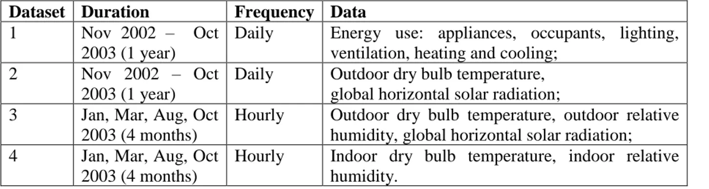
The validation datasets were historic data recorded for the reference house for the year 2002 – 2003. Table 2.2 summarizes the duration and frequency of the available data. They were provided by National Research Council Canada responsible for operating the facility. The measurement accuracy, however, is unclear due to the replacement of measuring devices and staff in charge. Therefore, the measurement error is not further discussed in this work.
Table 2.2: Summary of available measurements Dataset Duration Frequency Data 1 Nov 2002 – Oct
2003 (1 year)
Daily Energy use: appliances, occupants, lighting, ventilation, heating and cooling;
2 Nov 2002 – Oct 2003 (1 year)
Daily Outdoor dry bulb temperature, global horizontal solar radiation; 3 Jan, Mar, Aug, Oct
2003 (4 months)
Hourly Outdoor dry bulb temperature, outdoor relative humidity, global horizontal solar radiation; 4 Jan, Mar, Aug, Oct
2003 (4 months)
Hourly Indoor dry bulb temperature, indoor relative humidity.
A preliminary data processing was carried out and some missing data points were filled for the furnace gas and electric use measurement. The most significant problem was found in the weather data: the daily temperature means of Dataset 3 show significant differences with the available daily means from Dataset 2 in Table 2.2. Therefore, external weather data files for 2002 and 2003 were obtained for reference from WhiteBox Technologies for the Ottawa airport (WhiteBox Technologies, 2018).
Figure 2.2 shows the comparison of daily average ambient temperature between WhiteBox Technologies and the hourly measured values. We can see that the two data sets match quite well. To quantify the differences in the ambient temperature data, the heating and cooling degree days were calculated for both sets of data (when available) using a base temperature of 21 °C. The difference between the two datasets is less than 0.5 %.
Figure 2.2: Daily average ambient temperature - weather data file vs. measured values The agreement with hourly data is not perfect, but the daily averages are consistent with the recorded ones for all days. The match for solar radiation is not as good, as shown in Figure 2.3.
Figure 2.3: Global horizontal solar radiation - weather data file vs. measured values Solar radiation in the weather file is estimated from satellite measurements, so the accuracy can be expected to be lower. Solar radiation is also more complex to measure, so on-site
measurements could also present some inconsistencies. The total global horizontal solar radiation (integrated over the periods when measurements are available) is 93 % of the measured value. Figure 2.4 shows a 10-day period in summer where the agreement between both sets of data is very good. The satellite-based estimation is less accurate for cloudy days but provides a reasonable estimate of daily solar gains.
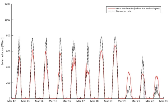
Figure 2.4: Global horizontal solar radiation - weather data file vs. measured values (August) Figure 2.5, on the other hand, shows a period in March where the weather data file consistently underestimates solar radiation for 8 days and then shows variations that bear little resemblance to the measured data.
Given the above analysis, a hybrid weather data file was adopted. The measured solar radiation was used when available while the outdoor dry bulb temperature was from WhiteBox Technologies since the difference is minor. This means that the differences shown in the above figures for solar radiation have been cancelled in the simulation. The solar radiation in the WhiteBox Technologies weather data for the other months cannot be verified, and it probably represents a relatively crude estimate of the actual solar radiation at the CCHT site. This may import considerable uncertainties to the calibration accuracy given that large south-facing windows are installed in the houses.
Figure 2.5: Global horizontal solar radiation - weather data file vs. measured values (March)
2.2 Methodology
2.2.1 Calibration criteria
In the literature, three guidelines were mentioned for calibration criteria: the International Performance Measurement and Verification Protocol (IPMVP), the U.S. Federal Energy Management Program (FEMP) M & V guidelines and ASHRAE guideline 14-2014 (ASHRAE, 2014). The last two guidelines propose consistent criteria, which are employed as the calibration criteria in this study. The equations below explain the procedure to calculate the two main indicators Normalized Mean Bias Error (NMBE) and Coefficient of Variation of the Root Mean Squared Error (CVRMSE).
The Root Mean Squared Error (RMSE) is an absolute value in the variable units (e.g. kWh for energy use). In the equations below, 𝑦 denotes the simulation value while 𝑦𝑚 the measured value. 𝑦̅𝑚 denotes the average value of the N measurements.
𝑅𝑀𝑆𝐸 = √∑(𝑦 − 𝑦𝑚) 2 𝑁 − 1
The RMSE can be normalized by dividing it by the average value of the measured variable and expressed in %. This is usually referred to as the Coefficient of Variation of the RMSE (CVRMSE): 𝐶𝑉𝑅𝑀𝑆𝐸 = √∑(𝑦 − 𝑦𝑚)2 𝑁 − 1 𝑦̅𝑚 × 100% (2.2)
The RMSE is an unsigned value, so it does not indicate whether a model has a bias error. The Mean Bias Error can be used for that purpose. It is again a value expressed in the same units as the variable:
𝑀𝐵𝐸 =∑(𝑦 − 𝑦𝑚) 𝑁 − 1
(2.3)
The MBE can be normalized by dividing the value by the average of measured values, as for the CVRMSE. This gives the Normalized Mean Bias Error (NBME), expressed in %:
𝑁𝑀𝐵𝐸 = ∑(𝑦 − 𝑦𝑚)
(𝑁 − 1) × 𝑦̅𝑚 × 100%
(2.4)
The first three columns of Table 2.3 summarizes the recommended calibration criteria by the ASHRAE guideline 14 to assess the uncertainty of the model. It only provides targets for the monthly and hourly calibration but not for daily calibration. It is reasonable to estimate that the targets for daily values would be between the targets for monthly values and for hourly values as shown in the last column of Table 2.3.
Table 2.3: Criteria of calibrated building energy models
Indicators Monthly Hourly Daily
NMBE 5% 10% 5%~10%
CVRMSE 15% 30% 15%~30%
2.2.2 Model inputs assumptions
The CCHT houses, unlike most calibration case studies, have rich reported information in relative reports and research papers; however, the presence of conflicting information is not
uncommon. The obtained data for internal gains, for example, are significantly different from the theoretical schedules presented in CCHT documents.
The method for selection and assumptions of the model inputs are based on the following steps: • literature review: a thorough literature review is conducted to collect all reported
information available about the houses. The information is then categorized in tables in order to identify the most possible value for each input. For instance, the value occurring most frequently is ranked as more trustworthy;
• on-site visits and meetings with colleagues from Natural Resources Canada: photos of houses and HVAC systems have been taken during the visits; a large part of the data and documents have been verified with on-site project managers;
• email verification: emails are exchanged for further verification during the course of the calibration process;
• engineering judgment: experience from engineering practice is the last resort to assume certain inputs for unconfirmed information.
Finally, when the uncertainty of input parameters is high or the input information unavailable, for example, the soil properties used for basement modelling is unknown, some alternative values are explored within boundaries to improve the model performance.
The iterative process of calibration is manually conducted. The optimization method is not employed because the model of the initial version has a good performance basis before the calibration. Optimization may pose a risk to overfit the model to the data. When simulation results of the model reach within the set criteria, no further improvement is explored to reduce the gaps between the simulation and the measurements.
A sensitivity analysis of some key input assumptions is further carried out after the calibration.
2.3 Detailed modelling in TRNSYS
In this work, TRNSYS was employed to model the building system based on first principles (Thermal Energy System Specialists LLC, 2018). This software has been certified based on ASHRAE standard 140 (ASHRAE, 2014) and accepted for certifications such as LEED and
ASHRAE standard 90. The sections below explain the essential components of the whole building model.
2.3.1 Zones and constructions
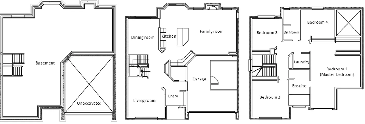
Figure 2.6 presents the sketch of floor plans with room separations. Type 56 (TrnBuild), a multi-zone building module in TRNSYS, uses the concept of thermal multi-zones by assuming a homogeneous air temperature across a zone. Therefore, zoning scenarios in a Type 56 model may not be identical to the real world room separations. In the final model, a 3-zone scenario was used by regarding each floor as a thermal zone with open doors: the first floor, the second floor, and the basement. The garage and attic are always included as two separate zones in the model to account for the thermal interaction between conditioned and unconditioned zones.
Figure 2.6: Floor plans of the CCHT houses
Type 56 requires data of construction properties including conductivity, specific capacity and density of layers composed of the building structures as well as the geometry of enclosed spaces. This information was taken from the as-built engineering drawings of the houses.
Equivalent layers of the wood studs were calculated using thermal properties from the literature. In particular, the thermal conductivity for insulation batts is assumed to be 0.046 W/m-K (ASHRAE Fundamentals 2009 Chapter 18), which leads to thermal resistance RSI values for the walls that are significantly lower than the “nominal” values mentioned on the as-built drawings. For example, nominal RSI value of the insulation layer mentioned in the drawings is 3.85 m²-K/W; the actual RSI value for the insulation layer, with a thickness of 140 mm and a conductivity of 0.046 W/m-K is 3.04 m²-K/W or 79 % of the nominal value.
The window type in the model uses an equivalent window, which assumes an identical window type with overall U-value 1.73 W/m²-K for all the windows in the house. The window area is then assigned for each window in the zones.
2.3.2 Basement
Basement is an important part in the residential house modelling, as it introduces a significant uncertainty in the heat transfer between the building and the ground. Type 1244 (Thornton et al., 2018) was adopted in the whole building model for the interaction between the ground and building parts in contact with it (e.g. basement and garage slab). This type requires physical parameters of soil and the environment (e.g. soil density, soil specific heat, and the day of minimum surface temperature), as well as geometry information and heat transfer rates from the building to the surrounding ground.
Type 1244 uses a 3D array to map the geometry of the built volume and the defined surrounding space. It divides the given building geometry and maximum distances beyond the building in multiple 3D cells. The elements of the array do not necessarily represent volumes of the same size. The closer to the boundaries, the smaller. The contents of the array indicate the volume to be inside of one of the building zones, above or in the ground.
The CCHT house has two building zones: the garage slab, and the basement. Considering all the detailed dimensions for the basement, the resulting array has 60 × 51 × 15 cells along the three dimensions (𝑥, 𝑦, 𝑧). The first horizontal layer (𝑥, 𝑦) of the array is shown in Figure 2.7, where the global shape of the house (see in Figure 2.6) can be recognized. The yellow color represents the basement and the red color represents the floor in contact with the garage. The z-axis is represented as successive layers in the text file.
Clay type soil parameters are taken in the model and are listed below. The uncertainty on most of these parameters is relatively high, so alternative values were explored in the calibration process. A brief sensitivity analysis can be found in section 2.4.3.
Table 2.4: Type 1244 (3D ground coupling) parameters
Parameter Value Units
Soil thermal conductivity 1.9 (values between 1 and 2.4 were explored) W/(m-K) Soil density 1930 (values between 1900 and 2400 were
explored) kg/m3
Soil specific heat 0.84 kJ/(kg-K)
Deep earth temperature 8.3 (values between 5.8 and 8.9 °C were explored) °C Amplitude of surface
temperature
14.2 (value between 12 and 14.2 °C were
explored) °C
Day of minimum surface
temperature 41
Day of the year
Soil surface mode 1 -
Soil surface emissivity 0.90 -
Soil surface absorptance 0.40 -
2.3.3 Infiltration and HRV
The infiltration model used in the study was the Alberta Infiltration Model (AIM-2). The AIM-2 (Walker & Wilson, 1998) model only applies to detached single-family buildings up to 3 storeys. It implements a simple natural ventilation algorithm with empirical functions for the superposition of wind and stack effect. Furnace, fireplace and Domestic Hot Water (DHW) flues are considered as separate leakage sites. The model differentiates houses with basements (or slab-on-grade) and crawlspaces. Parameters from the blower door test of the CCHT houses were used in the model.
A Heat Recovery Ventilation (HRV) unit was installed in the houses and Type 760 in TRNSYS was used to model this unit. Figure 2.8 shows the schematic of the ventilation system in the TRNSYS model. Part of the return air goes through the HRV and then mixes with the rest of the return air before entering the furnace system.
Figure 2.8: Diagram of a forced air system with HRV
Constant air volume to each zone was assumed in the model with total flowrate 65 cfm with the defined ratio to each zone. The HRV power is set to a constant value of 94.5 W. The effectiveness of the HRV is assumed to vary linearly with the ambient temperature. The 2 points at 0 °C and -25 °C are taken from the HVI ratings for Venmar AVS HE1.8 at the lowest flowrate (Venmar, 2018), where Venmar was the original system installed in the reference house. The rated values at the two points are respectively 84 % and 72 %. Note that the effectiveness is not extrapolated, i.e. 84 % is kept above 0 °C, and 72 % is kept under -25 °C. The following equation is implemented in the model:
𝜀𝐻𝑅𝑉 = min ( 0.84, 𝑚𝑎𝑥 ( 0.72, 0.84 + 𝑇𝑑𝑏𝑎𝑚𝑏 ⋅0.12 25 ) )
(2.5)
Defrost is modelled in a simple way: if the ambient temperature is below -5 °C, the HRV switches to defrost mode for 12 min per hour, based on a fixed schedule. This means that the fresh air flowrate goes to zero and the fan power increases to 175 W. That heat is injected into the return air before the furnace.
2.3.4 Forced air system
As presented in Figure 2.8, the original system in the reference house is a forced air system, commonly seen in Canadian single-family homes. The conditioned air is supplied from the
basement to each zone through ducts with fresh air handled by the HRV system. The furnace uses gas as the main fuel source and shares the same blower fan with the air conditioner.
In the TRNSYS model, the furnace is modelled with a constant efficiency of 80.2 % and a capacity of 17584.3 W (60000 Btu/h). The setpoint for the supply air temperature is unknown. It is set to a high value (60 °C) in the model so that the supply air temperature is limited by the furnace capacity. The supply air temperature actually never reaches 60 °C in the simulation because the flowrate is high enough.
The air-conditioner is modelled with TESS Type 921. A TRNSYS performance map has been created from the manufacturer data. The rated conditions are taken from the performance map:
• Total cooling capacity = 6.86 kW
• Sensible cooling capacity = 5.14 kW (sensible heat ratio of 75 %) • Power use = 2.06 kW
• COP = 3.32
The power used by the condenser fan is assumed to be included in the data. The manufacturer data provides the motor horsepower 1/5 hp. Assuming a permanent split capacitor motor efficiency of 60 %, the actual power usage of the fan would be 250 W. This power is used in Type 921 but has no impact on performance as it is assumed to be included in the performance map.
The air handler flowrate and fan power are estimated as follows: • Low speed (circulation): 450 L/s, 350 W
• 2nd highest speed (heating): 620 L/s, 530 W • Highest speed (cooling): 680 L/s, 570 W
The power used for the furnace power vent motor is not explicitly taken into account (i.e. it is supposed to be included in the 530 W).
These 3 points are used to define a power curve for a variable speed fan. The control signal is adapted to the operation mode (circulation, heating, or cooling). In TRNSYS, this is implemented as follows:
Fan rated flowrate 2947.392 kg/h, fan rated power 2052 kJ/h Fan power curve:
𝑃 = −1.056445 + 3.439614𝑚 − 1.383168𝑚2 (2.6) 𝑚 is the flowrate in each mode and 𝑃 is the power.
Fan control signal (speed ratio):
𝑠𝑝𝑒𝑒𝑑𝑅𝑎𝑡𝑖𝑜 = 0.661765 + 𝑓𝑢𝑟𝑛𝑎𝑐𝑒𝑂𝑛 ⋅ 0.250000 + 𝑎𝑐𝑂𝑛 ⋅ 0.338235 (2.7)
2.3.5 Internal gains and occupancy
The appliances, lighting and occupant simulators in the CCHT houses were operated according to a predefined schedule repeated daily. Note that the occupants were simulated using lightbulbs, so there were no humidity gains. This experimental setting reduced the complexity of the calibration study associated with the accessory energy use. In the calibrated model, the schedule with measured power consumptions for all equipment was imported as external data into the model. Therefore, there are no differences between simulation results and measurements for the appliance yearly energy use.
For internal gains due to lighting, appliance, and occupants, they are split between convective and radiative parts according to standard ratios from the ASHRAE handbook fundamentals (American Society of Heating, Refrigerating and Air-Conditioning Engineers, 2017). The ratios of the internal gains that are actually released in the room are also referred from the handbook, e.g. for the dryer, most of the electricity (70%) is used to heat the exhausted air, which means only 30% becomes internal gains.
2.4 Calibration results
Since the calibration is an iterative process, different versions of TRNSYS models of the whole house were simulated with different parameters and inputs. All simulations during the process were run for 2 full years (2002 and 2003) with a time step of 5 minutes. The results reported here is the final version of the model, and results from November 2002 to October 2003 are used for comparison and analysis.
2.4.1 Energy use results
Yearly results
Table 2.5: Annual energy use, measured and simulated
Item Meas. values Model version r205 Comments MJ MJ % diff. Lighting and appliances 11577 11577 0.0%
Model inputs including lights and receptacles, fridge, stove, dishwasher, clothes washer, dryer
Furnace fan 12910 12375 -4.1%
Fan power at different speeds is model input, differences caused by operating hours in different modes
HRV fans 3054 3090 1.2% Fan power is model input, differences caused by operating hours in defrost mode
DHW blower 203 203 0.2% Blower power when operating is model input, differences caused by operating hours
Air
conditioner 5759 5729 -0.5%
Includes compressor power and outdoor fan power. Performance map is an input
Furnace gas 65701 65558 -0.2% Furnace steady-state efficiency is model input (80 %), differences caused by load differences DHW gas 25569 25630 0.2% Differences can be attributed to mains water
temperature Total
electricity 33503 32973 -1.6%
Differences mostly come from furnace air-handler power, somewhat compensated by other categories Total gas 91270 91188 -0.1% Relatively similar differences for furnace and DHW
(both slightly overestimated)
Total energy 124773 124162 -0.5% Obtained by summing gas and electricity MJ, without equivalence factors
Table 2.5 summarizes the annual energy use for each category with the second column showing the measured energy use. The third column lists the simulated energy use with the number r205 indicating the model version accepted as the calibrated model. Note that this number in the figures and tables below means the same final model version.
We can see that the error on total energy use (gas and electricity combined) is as low as 0.5 %. This includes lighting and appliances, which are model inputs and account for 10 % of the total
energy use. The relative error on annual energy use for heating and cooling are both less than 1 %. These differences could be even reduced by fine-tuning some of the parameters, but this was not attempted given the relatively high uncertainty on some key parameters e.g. Air Changes per Hour (ACH) @ 50 Pa. A discussion on the impact of some key parameters is presented in section 2.4.3.
Monthly results
Figure 2.9 presents the monthly energy use for heating (furnace gas) and cooling (air-conditioner electricity). Both values are expressed in MJ/day. It should be noted that the negative bars for cooling do not denote negative electricity use. The negative sign is only used as per the TRNSYS convention.
Figure 2.9: Monthly furnace gas and air-conditioner electricity use
We can find that the energy use differences of each month are within 10%. Larger differences are observed for January (underestimation) and for February and March (overestimation). The overestimation in February could be related to low solar radiation in the data file. The profile of the undisturbed ground surface temperature could also have an impact. The underestimation in October could be related to start-up problems or slight setpoint differences at the beginning of a new heating season.
The 𝐶𝑉(𝑅𝑀𝑆𝐸) of monthly energy use of the model are:
Furnace gas use: 𝐶𝑉(𝑅𝑀𝑆𝐸) = 7.9 % Air-conditioner electricity: 𝐶𝑉(𝑅𝑀𝑆𝐸) = 6.2 %
Both results indicate a good performance of the calibrated model, well under the ASHRAE target of 15 %. Note that the results here only count the heating season for furnace gas use and cooling season for air conditioner electricity use. The 𝑁𝑀𝐵𝐸 values of the model are also well under the ASHRAE target of 5% as shown below:
Furnace gas use: 𝑁𝑀𝐵𝐸 = −0.1 % Air-conditioner electricity: 𝑁𝑀𝐵𝐸 = −0.6 %
Daily results
Given that our measurements have daily energy use data for a full year, we compared the simulated daily energy use with the measurements, although daily results comparison are not required by the ASHRAE guideline. Figure 2.10 shows the daily values for furnace gas use and air-conditioner electricity use, while Figure 2.11 shows the daily errors for the same variables. Both values are in very good agreement. The day-to-day variability of heating and cooling demands seems to be well captured by the model. Figure 2.11 also identifies the data points that were interpolated in the experimental data. Some of the largest differences occur during interpolated days, which would seem to indicate that the procedure used to fill in missing daily values is at least partly responsible for these larger discrepancies. Some relatively large errors are still present during the non-interpolated days, and the model seems to consistently overestimate the heating load in late February / early March. However, most of the large errors are all within 20% of the absolute values for that particular day.
Figure 2.10: Daily furnace gas and air-conditioner electricity use
Figure 2.11: Daily error on furnace gas and air-conditioner electricity use
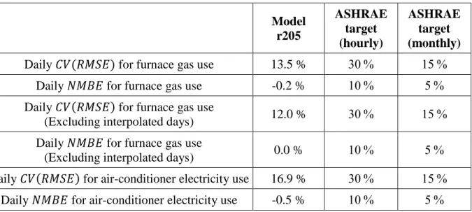
Table 2.6 shows the daily performance indicators and the ASHRAE targets. All performance indicators for daily energy use are well within the ASHRAE targets for hourly values and in most cases even within the targets for monthly values.
Table 2.6: ASHRAE goodness-of-fit indicators for daily energy use Model r205 ASHRAE target (hourly) ASHRAE target (monthly)
Daily 𝐶𝑉(𝑅𝑀𝑆𝐸) for furnace gas use 13.5 % 30 % 15 %
Daily 𝑁𝑀𝐵𝐸 for furnace gas use -0.2 % 10 % 5 %
Daily 𝐶𝑉(𝑅𝑀𝑆𝐸) for furnace gas use
(Excluding interpolated days) 12.0 % 30 % 15 %
Daily 𝑁𝑀𝐵𝐸 for furnace gas use
(Excluding interpolated days) 0.0 % 10 % 5 %
Daily 𝐶𝑉(𝑅𝑀𝑆𝐸) for air-conditioner electricity use 16.9 % 30 % 15 % Daily 𝑁𝑀𝐵𝐸 for air-conditioner electricity use -0.5 % 10 % 5 %
2.4.2 Dynamic results
Hourly values are available for the first floor, for selected periods. These values are plotted with hourly-averaged simulation results in Figure 2.12.
Figure 2.12: Room temperatures - hourly measured and simulated values
Hourly temperatures show significant variation within the margins of the controllers deadbands, due to the on/off nature of the heating and cooling control. The free-floating behaviour during
shoulder periods seems to be well reproduced by the model (early October 2003). The basement is significantly colder than the other floors, and this will be analyzed below.
The ASHRAE indicators can be calculated for the 4 months for which hourly measurements are available. The table below shows that the 𝐶𝑉(𝑅𝑀𝑆𝐸) for air-conditioner power usage is slightly above the ASHRAE target. Unfortunately, it is difficult to draw conclusions given that only one month of data (August) and a few days in October are available.
Table 2.7: ASHRAE goodness-of-fit indicators for hourly energy use Model
r205
ASHRAE target (hourly) Hourly 𝐶𝑉(𝑅𝑀𝑆𝐸) for furnace gas use 31.5 % 30 %
Hourly 𝑁𝑀𝐵𝐸 for furnace gas use -3.7 % 10 %
Hourly 𝐶𝑉(𝑅𝑀𝑆𝐸) for air-conditioner electricity use 38.7 % 30 % Hourly 𝑁𝑀𝐵𝐸 for air-conditioner electricity use -2.3 % 10 % Hourly 𝐶𝑉(𝑅𝑀𝑆𝐸) for room temperature 1.8 % 30 %
Hourly 𝑁𝑀𝐵𝐸 for room temperature -0.4 % 10 %
The next figures show more details on the dynamic behaviour, plotting the 5-min simulated values against hourly measured values for typical periods in winter and summer.
Figure 2.13 shows a typical cold winter week. The on/off furnace control leads to large oscillations around 21 °C for the main floor, while the second floor is generally slightly warmer and the basement is significantly colder (but with similar oscillations as their flowrate is controlled simultaneously). Even during very cold periods, the furnace rarely turns on for two consecutive time steps with the selected deadband. During periods with higher gains, the furnace sometimes remains off for several hours.
The average measured main floor temperature (hourly measurements are only available for two months) is 21.1 °C, while the average simulated 1st-floor temperature over the same period is 21.07 °C. The measured temperature corresponds to one point (thermostat location), while the simulated value models the volume average of the entire floor, so this good match hides differences such as the ones visible in Figure 2.13 during the high gain periods.