An alternative approach to alternative beta

Thierry Roncalli

_{J´erˆome Te¨ıletche}

April 2007

Abstract

Hedge fund replication based on factor models is encountering growing interest. In this paper, we investigate the implications of substituting standard rolling windows regressions, which appear ad-hoc, with more efficient methodologies like the Kalman filter. We show that the copycats constructed this way offer risk-return profiles which share several characteristics with the ones posted by hedge funds indices: Sharpe ratios above buy-and-hold strategies on standard assets, moderate correlation with standard assets and limited drawdowns during eq-uity downward trends. An interesting result is that the shortfall risk seems less important than with hedge fund indices and regressions based-trackers. We finally propose new breakdowns of hedge fund performance into alpha, traditional beta and alternative beta.

Hedge fund replication has become highly fashionable during recent months. Under this generic term, three main approaches can be identified:

• Mechanical duplication of strategies. A growing number of investment banks are proposing

products which aims to reproduce in a systematic and quantitative manner a strategy followed by hedge funds. For instance, several investable indices have been proposed which mark-to-market systematic short of put options or variance swaps. Thanks to the positive premia between implied and realized volatilities, this kind of strategy seems able to generate superior Sharpe ratios while exposing to the risk of huge losses when the underlying asset plunges (Lo [2005], Goeztmann et al. [2007]). Other candidates include trend-following strategies, i.e. CTA/managed futures, which can be mimicked through lookback straddles (see Fung and Hsieh [1997]), merger arbitrage strategies which can be replicated by passive investments in all announced mergers (Mitchell and Pulvino [2001]), fixed income funds that Fung and Hsieh [2002] have shown to be reproducible through credit exposure and constant-maturity products, long-short equity which can be mimicked through beta-one plus small vs large caps exposures, convertible arbitrage (Agarwal et al. [2006]) or, for Global Macro, systematic FX carry strategies. All in all, Fung and Hsieh [2007] estimate that 75% of net assets of hedge fund are covered by this type of systematic strategies.

• Replication of distribution. A very different approach has been advocated by Kat and

Palaro [2007]. Their postulate is that investors enter into hedge funds for their character-istics in terms of expected returns, volatility and correlation, not for their month-by-month return. While the argument might be generalized to other assets, it is probably all the more meaningful as diversification is a major motivation for investing in hedge funds. In practice, the copycat is based on a passive futures trading strategies1_{. The investor first determines} its existing portfolio (for instance, an equally-weighted mix of US Treasuries and S&P 500), the futures he wants to trade and then the statistical properties in terms of correlation with the existing portfolio, shortfall probability, skewness sign, etc. The investor then receives the

above all, this is based on the strong implicit assumptions that correlation among underlying futures is constant through time.

• Factor-based model. This approach relies on linear regressions of hedge fund returns on a

list of market factors, being representative of long-only or spread exposures of hedge funds (equity, credit and bond indices; value/growth spread, small/big caps spread, etc.). A large empirical literature has studied this form of models; see, among many others, Fung and Hsieh [1997,2004], Hasanhodzic and Lo [2006], Jaeger and Wagner [2005], Agarwal and Naik [2004]. Results appear to be mixed and highly different depending on strategies: while directional strategies (equity hedge, emerging markets, global macro) present strong exposures, pure market-neutral/arbitrage ones naturally show limited exposures. Despite these mixed results, the hedge fund industry seems to be largely exposed as a whole, mainly because of the dominant market share of long/short strategies. For instance, based on monthly returns, the correlation of the HFR index with the S&P 500 index is more than 70% over the period 1990-2006. This evidence has led to the expression “alternative beta” which denotes the part of the hedge fund returns that can be attributed to directional investments in standard assets. One huge difference between alternative beta and traditional beta is that for hedge funds, exposure is not a passive one but should integrate non-linear effects. For instance, as they follow dynamic strategies, hedge funds regularly change their exposure, which gives rise to option-like payoffs2_{. To deal with these features, authors have incorporated measures} of option payoffs such as long systematic position in straddles.

These approaches differ in various dimensions. The first two seem more ambitious in that they hope to generate synthetic clones whom performance will be similar to the one (gross of fees) of hedge funds. The last approach simply promises to get the fraction of hedge fund returns which can be linked to the alternative beta, that is to their varying exposures – including the possibility of shorting – to the standard assets. In this perspective, part of the hedge fund alpha is attributed to this dynamic switching between assets. But all the alpha cannot be reproduced as alpha can stem from investing in illiquid securities or ultra-high frequency trading and thus not reproducible through low frequency trading in liquid futures. Later in this article, we try to disentangle hedge fund returns into alpha, alternative beta and traditional beta in a more precise way. While this approach appears less ambitious, it has clear advantages on top of which simplicity, transparency and cost-effectiveness. On the contrary, as they aim to replicate complicated hedge fund strategies, the first two approaches expose itself to operational risks, black-box criticisms or (possibly) high trading costs3_{. Thus, if the major objective is to get higher transparency, lower} regulatory constraints or liquidity, one should concentrate on the factor-model approach. In this perspective, it is not surprising that, to date, this methodology has been the most widespread. Still, most existing approaches has in common a deficiency: they are based on OLS regressions over rolling windows whose time-lag is determined in an ad-hoc fashion. More efficient econometric techniques are available such as the Kalman filter. This paper investigates whether more robust alternative betas processes can be built using such techniques4_.

The rest of the paper is as follows. In Section 2, we describe the rolling OLS and the Kalman filter and illustrate their differences through examples. In Section 3, we analyze their difference when applied to the alternative beta issue. In Section 4, we present some applications of Kalman filter alternative betas concept. First, we analyze their properties as investment vehicles, comparing them with standard hedge fund investments. Second, we propose new decompositions of hedge fund performances into alpha and beta components. Conclusions are drawn in Section 5.

2_{In an early analysis, Merton [1981] showed that a manager pursuing a strategy of market timing between} several assets is likely to generate similar returns to those of an optional position on one of the assets without nonetheless taking up a position on options.

3_{Even in the case of the approach of Kat and Palaro [2007] which is based on liquid futures, the tailor-made} specification for each investor makes the minimum investment size very high due (at least EUR 20 Mns according to information dissiminated on the FundCreator website).

4_{Another promising approach has been advocated by Darolles and Mero [2007]. Building on the methodology} developed by Bai and Ng [2002, 2003], the authors estimate latent factors models from a large sample of individual funds. After extracting the number of appropriate factors, they identify them with standard market factors.

1

Kalman filter and dynamic allocation

1.1

Recovering dynamic allocation

Let Rt and Ft(i) be respectively the return of the hedge fund strategy and the returns of the i

individuals factors (i = 1, . . . , m) at time t. We have:

Rt= m

X

i=1

w(i)t Ft(i) t = 1, . . . , T

with wt(i)the weight of the ithindividual strategy. The issue is to recover the time-varying allocation

w(i)t . We may solve this problem by estimating the local beta of the portfolio with respect to the

individual strategies. The regression might or not include an intercept, an aspect we discuss below. 1.1.1 With rolling OLS

One of the most used technique to recover dynamic allocation is the rolling OLS method. In this case, we assume a linear model: Rt =

Pm i=1β(i)F

(i)

t + ut and the estimates ˆw(i)t correspond to

the OLS estimation of β(i) _{on the period [t − h, t] where h is the rolling window. For instance,} Hasanhodzic and Lo [2006] use a 24-months lag window. Note that we may use the QP method described in AppendixAto impose some constraints (e.g.¯¯β(i)¯_{¯ ≤ 1) or to center the residuals in} the case where no intercept is included into the regression.

1.1.2 With Kalman filter

An alternative approach is to use the Kalman filter described in AppendixBwith the model:            Rt = P_m i=1β (i) t Ft(i)+ ²t βt(1) = βt−1(1) + ηt(1) .. . β(m)t = βt−1(m)+ ηt(m) (1) where ²t ∼ N ¡ 0, σ2 ² ¢ and η(i)t ∼ N ¡ 0, σ2 i ¢

are uncorrelated processes. Using the notations in-troduced in the appendix, the state-space form is Zt=

³

Rt(1) · · · R(m)t

´

, ct = 0, Ht= σ²2,

Mt= Im, dt= 0, St= Imand Qta diagonal matrix such that:

Qt=    σ2 1 0 . .. 0 σ2 m   

We assume moreover that P0 = 0m. It means that we know exactly the initial allocation. We

will later discuss this point. We denote θ the vector of parameters to be estimated by maximum likelihood with θ =¡ σu σ1 · · · σm

¢

. More details concerning estimation and the Kalman filter methodology.are given in Appendix B.

1.2

Some examples

Let us consider an example to illustrate the difference between both methods to evaluate the exposures5_{. We suppose a strategy corresponding to a monthly dynamic allocation between MSCI} USA and MSCI EMU since 1990. We assume that the weights are oscillating and are given by_{¡ ¢}

Figure 1: KF estimates versus Rolling OLS estimates – $ = 5Y

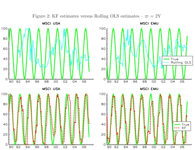
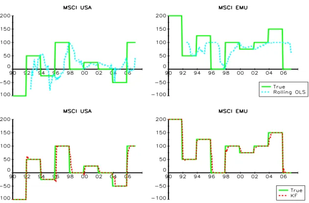
Figure 3: KF estimates versus Rolling OLS estimates – $ = 2Y

Let us now consider a more realistic example. We assume that weights change by step of 25%, with wU SA

t = (w ⊗ 1 )t and wEM Ut = 1 − wtU SA for w = (−1, 0.5, −0.25, 1, 0.25, 0, −0.5, 1, . . .).

The portfolio is 100% long with the possibility of being short in one asset. Results are reported in Figure3. One criticism is that state vector estimates might be too much dependant on initial values. But in practice, this is not truly the case as shown in Figure4. Indeed, one of the properties of the Kalman filter is its high ability to quickly adapt to changing conditions.

It is interesting to remark that because P0= 0m, the estimates btand bt|t−1are homogeneous

with respect to the vector of parameters θ, that is they do not change if θ is scaled by a factor κ. To show this property, we remark that if Q∗_{= κ}2_{Q and H}∗_{= κ}2_{H, it comes that P}∗

t|t−1= κ2Pt|t−1,

F∗

t = κ2Ft and Pt∗ = κ2Pt. We also have P∗_t|t−1Zt>Ft∗−1 = Pt|t−1Zt>Ft−1, so we prove that

b∗

t|t−1 = bt|t−1 and b∗t = bt. Moreover, we may show that the state vector is invariant if we both

scale Rt, Ft(i) and ut. It means that the interested parameters are the ratios σ2/σ1, . . . , σm/σ1. These ratios give us a direct measure of the dynamic property of the allocation on the individual strategies. Bigger are these ratios, more dynamic is the allocation.

2

A comparison of OLS and Kalman filter when applied to

hedge fund replication

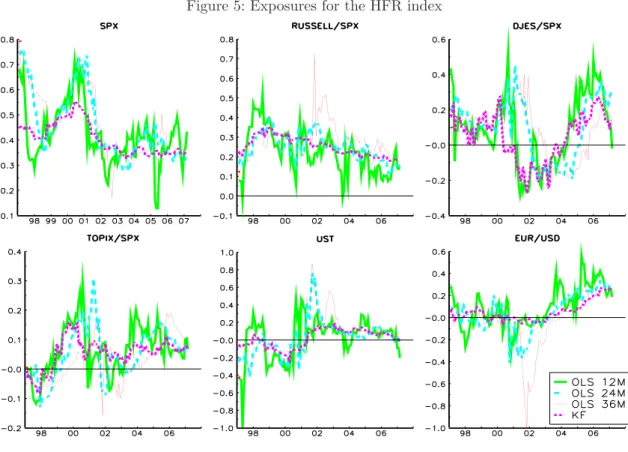
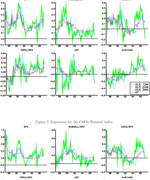
We try to estimate the beta using the following six underlying exposures:

1. an equity position in the S&P 500 index,

2. a long/short position between Russell 2000 and S&P 500 indices,

3. a long/short position between Eurostoxx 50 (hedged in USD) and S&P 500 indices,

4. a long/short position between Topix (hedged in USD) and S&P 500 indices,

5. a bond position in the 10-years US Treasury,

6. a FX position in the EUR/USD.

These exposures have been chosen as they correspond to standard exposures identified in the literature (see Agarwal and Naik [2004],Amenc, El Bied and Martellini [2003], Gehin and Vaissie [2006], Hasanhodzic and Lo [2006], Fung and Hsieh [2007], Jaeger and Wagner [2005]) but where we limit ourselves to liquid futures markets. For instance, we do not include any options or OTC swaps and exclude credit indices for which futures have been recently launched but are not enough mature to be included in this context. The models are estimated over the period 1994-2007 and are done on three well-known indices for matter of comparisons: the Composite HFR index, the HFR Funds-of-Funds index and the CSFB-Tremont total index. All of these indices are non-investable, which increase the interest for the exercise of replication here established. To make the backtest more reliable, we incorporate a lag of one month for incorporating the delays in release of indices.

We have estimated the dynamic beta using the rolling OLS technique for various frequencies (12 months, 24 months, 36 months) and the Kalman filter6_{. Results of the estimations are reported} in Figures 5, 6 and 7. We observe that whatever the methodology which is used, hedge funds considered as a whole have appeared as long equities as a whole - as captured by the S&P7 _{- and}

5_{See Swinkels and Van der Sluis [2006] for a more in-depth analysis in the context of style-based analysis.} 6_{One should notice that the parameters of the Kalman filter are estimated over the whole sample. However, here,} it is not the coefficients but only their variance which are estimated. It is not clear whether this implies look-ahead bias and in practice, we have found that progressive estimations of the Kalman filter are leading to very similar results. Readers familiar with Kalman filter indices should not be surprised with this result.

7_{The aggregated exposure to the S&P index should be read as the sum of the ”S&P” exposure (as mentionned} in the figure) minus all the exposures of spreads involving the S&P. In fact, the exposure mentionned as ”S&P” recovers the total equity exposure.

long Russell against S&P. For other factors, exposures vary to a large extent between methods. Still, whatever the factor and the index publisher which are considered, the variability of exposures is far lower for the Kalman filter. Obviously, as one is attempting to capture the dynamic beta of hedge fund, stability is not an objective as such. But it is not clear whether it is efficient to have quickly changing exposures if true underlying exposures are themselves highly volatile. Indeed, in this case, the danger is to be always “behind the curve”. For instance, there seems to have been numerous inopportune changes in exposures for the 12 months window, as for instance the large decrease in exposure to S&P in end 1997 or the sharp changes in exposures in 2004/2005. At the other end of the spectrum, a too long window can lead to react too slowly to changing conditions, as is magnified here by the S&P exposure during the collapse of the stock market bubble and the recovery period which has followed. Undeniably, the Kalman filter appears as a good compromise: it posts smooth changes in exposures but has been able very early (even earlier than the 12 months rolling window) to identify the reduction in exposure to equities markets which seems to have characterized hedge funds in late 2000-early2001.

Figure 5: Exposures for the HFR index

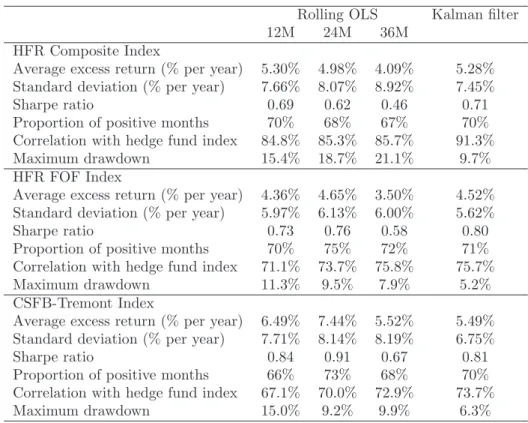
More formally, we report in Table 1 some statistics on the simulated returns of the various methodologies. It appears that while some lag windows lead to higher average excess returns than the Kalman filter method, none globally dominates the latter in terms of risk-adjusted returns. As far as capital preservation is concerned, the Kalman filter also seems to be preferred as it often leads to an higher proportion of positive months and systematically to lower drawdowns. Finally, it offers an higher correlation with the underlying hedge fund index.

Figure 6: Exposures for the HFR FoF index

Table 1: Descriptive statistics on simulated factor models

Rolling OLS Kalman filter 12M 24M 36M

HFR Composite Index

Average excess return (% per year) 5.30% 4.98% 4.09% 5.28% Standard deviation (% per year) 7.66% 8.07% 8.92% 7.45% Sharpe ratio 0.69 0.62 0.46 0.71 Proportion of positive months 70% 68% 67% 70% Correlation with hedge fund index 84.8% 85.3% 85.7% 91.3% Maximum drawdown 15.4% 18.7% 21.1% 9.7% HFR FOF Index

Average excess return (% per year) 4.36% 4.65% 3.50% 4.52% Standard deviation (% per year) 5.97% 6.13% 6.00% 5.62% Sharpe ratio 0.73 0.76 0.58 0.80 Proportion of positive months 70% 75% 72% 71% Correlation with hedge fund index 71.1% 73.7% 75.8% 75.7% Maximum drawdown 11.3% 9.5% 7.9% 5.2% CSFB-Tremont Index

Average excess return (% per year) 6.49% 7.44% 5.52% 5.49% Standard deviation (% per year) 7.71% 8.14% 8.19% 6.75% Sharpe ratio 0.84 0.91 0.67 0.81 Proportion of positive months 66% 73% 68% 70% Correlation with hedge fund index 67.1% 70.0% 72.9% 73.7% Maximum drawdown 15.0% 9.2% 9.9% 6.3%

3

Application to alternative beta

3.1

Building a clone

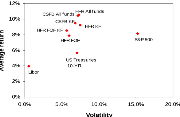
To evaluate whether factor-models replicating funds are worth investing in, we report in Figure8

the backtest of the strategy over the period 1997-2007 (with cash reinvested in Libor). In Figure9, we compare the risk-return profile (in terms of mean-variance). More statistics are given in Table

2. Several comments are worth stressing.

First, concerning composite indices of single funds, the trackers post underperformance in face of the indices they try to replicate, despite their fairly high correlation. But perfect replication seems to be an unfair objective in the present case. It is well-known that hedge fund indices are affected by various biases: survivorship bias, self-selection bias8_{. An indication of the validity of} this explanation is that this result does not hold for the Funds-of-Funds replication. Indeed, it is widely acknowledged that the returns of Funds-of-Funds are less affected by those biases since, for instance, they do not cease reporting to database when an underlying single fund in which they have invested collapse but their NAVs are directly impacted. Obviously, one should keep in mind that the difference in performance between single funds and funds-of-funds also reflect the additional layer of fees. By and large, it seems that over a full economic and market cycle (that is the last 10 years), trackers post performances which are characteristic of hedge fund performance with a slight underperformance probably due to the lack of alpha generation (an issue on which we return later).

Second, an attractive feature visible in the results is that trackers present larger skewness than the indices. This positive asymmetry shift is also clear when one observes the extrema since trackers exhibit lower minima and higher highs. While it is beyond the purpose of the present paper to deal with this issue, an explanation for this result is that, by construction, factor-based models are getting off strategies similar to writing puts on the market9_{. This would act as a recommandation} to be cautious in introducing option payoffs in factor-based trackers.

Third, we can argue on the standard criticism directed at regression-based trackers that their correlation with equities is high. This is undeniably true but the correlation seems to mainly simply reflect the one of the indices they are tracking. In this perspective, it is interesting to notice that the correlation of the CSFB-Tremont tracker with the S&P 500 index is far lower than the one of its HFR counterpart, which is totally consistent with the respective correlation of the indices10_. We also notice that this correlation preservation is also observed for US Treasuries.

Table 2: A statistical comparison of hedge fund indices and their trackers

HFR HFR FOF CSFB-Tremont Index Tracker Index Tracker Index Tracker Average return (% per year) 10.5% 9.2% 7.9% 8.5% 10.4% 9.5% Standard deviation (% per year) 7.3% 7.5% 6.0% 5.7% 7.2% 6.8% Sharpe (risk-free rate = 4%) 0.90 0.71 0.66 0.81 0.90 0.81 Proportion of positive months 69.7% 69.7% 65.6% 71.3% 72.1% 70.5% Skewness -0.43 0.03 -0.25 1.01 0.18 0.52 Excess kurtosis 3.20 2.42 4.73 5.21 4.04 2.40 Minimum -8.70% -7.12% -7.47% -3.57% -7.55% -4.98% Maximum 7.65% 8.99% 6.85% 9.01% 8.53% 8.86% Correlation with S&P 500 72.0% 69.6% 52.9% 55.4% 48.7% 61.4% Correlation with US Treasuries -17.2% -14.5% -12.4% -5.1% -2.7% 3.5% 8_{See for instance Fung and Hsieh [2004] or Lhabitant [2006].}

9_{Evidence on this subject is large; see among others Mitchell and Pulvino [2001] or Naik et al. [2004].}

10_{The higher correlation of the HFR index is often attributed to the heavier weight of equity-linked strategies} (notably Equity hedge).

Figure 8: Backtest of the strategy 75% 100% 125% 150% 175% 200% 225% 250% 275% 300% 1997 1998 1999 2000 2001 2002 2003 2004 2005 2006 2007

Kalman filter (HFR index)

Kalman filter (CSFB-Tremont index) HFR FoF

Kalman filter (HFR FOF index) HFR All funds

CSFB All funds

Figure 9: Risk-return profile of hedge funds and standard assets

0%

2%

4%

6%

8%

10%

12%

A

v

e

ra

g

e

r

e

tu

rn

3.2

Estimating the Alpha

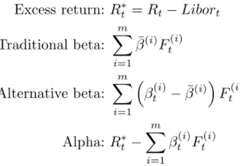
With the previous framework, it is easy to compute the various components of the hedge fund performance. Obviously, the calculations can be crude at best since, in practice, one should take into account the impact of fees and above all of the bias affecting the first moment (average) of hedge fund indices. Let Rtdenote the index monthly return observed at time t. βt(i)is the exposure

to the i-th factor as estimated through the Kalman filter and ¯β(i) _{is its average over the whole} period, ¯β(i)_{= T}−1PT

t=1β

(i)

t . Our aim is to decompose the total performance into fixed-traditional

beta, alternative beta and alpha. We adopt the following breakdown: Excess return: R∗t = Rt− Libort

Traditional beta: m X i=1 ¯ β(i)Ft(i) Alternative beta: m X i=1 ³

β(i)_t − ¯β(i)´_F(i)

t Alpha: R∗ t− m X i=1 β_t(i)F_t(i)

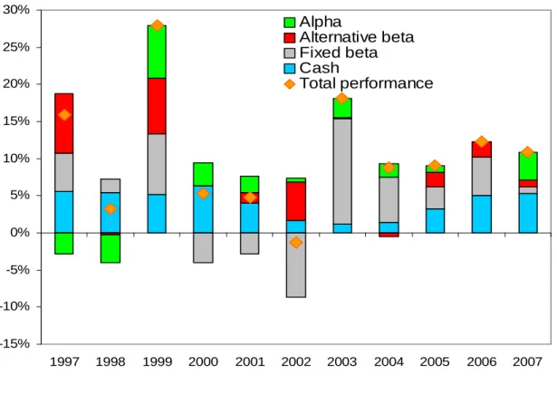
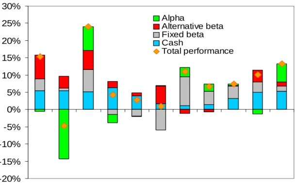
In Table3, we report the average values obtained for each of these components. For the various indices, alternative beta does represent between a quarter and a third of the total return and near one-half of the excess return. In Figures 10, 11 and 12, we report the same calculations but for every year. It is interesting to observe that alternative beta has contributions to performance which are most of the time positive and that their contribution was the most important during the bear equity market (2002 and to a lesser extent 2001).

Table 3: Decomposition of the total return of hedge fund indices (January 1997 – February 2007) (% per year) HFR Composite CFSB-Tremont HFR FOF

Total performance 10.39% (100.0%) 10.30% (100.0%) 7.87% (100.0%) Cash 3.92% (37.7%) 3.92% (38.1%) 3.92% (49.8%) Traditional beta 2.79% (26.8%) 2.39% (23.2%) 2.02% (25.6%) Alternative beta 2.49% (24.0%) 3.09% (30.0%) 2.51% (31.8%) Alpha 1.19% (11.4%) 0.90% (8.7%) -0.57% (-7.2%)

4

Conclusion

Hedge fund replication meets growing interest. As far as the motivation is to get liquid and trans-parent instruments, factor-models appear as an attractive approach. To date, though, available approaches are based on rolling regressions where the window is fixed in an ad-hoc way. In this paper, we have shown that more efficient econometric methods such as the Kalman filter can be used as substitutes to these regressions. They offer risk-return profiles which share several charac-teristics with the ones posted by hedge funds indices: Sharpe ratios above buy-and-hold strategies on standard assets, moderate correlation with standard assets or limited drawdowns during equity downward trends. An interesting result is that the shortfall risk seems less important than with hedge fund indices. All in all, alternative beta appear to explain between a quarter and a third of the total performance of hedge funds.

References

[1] Agarwal, V., W. Fung, Y-C. Loon and N. Naik [2006], Risk and return in convertible ar-bitrage: Evidence from the convertible bond market, London Business School Working Paper.

Figure 10: Year by year decomposition of the performances for the HFR index -15% -10% -5% 0% 5% 10% 15% 20% 25% 30% 1997 1998 1999 2000 2001 2002 2003 2004 2005 2006 2007

Alpha

Alternative beta

Fixed beta

Cash

Total performance

Figure 11: Year by year decomposition of the performances for the CSFB-Tremont index

-5% 0% 5% 10% 15% 20% 25% 30%

Alpha

Alternative beta

Fixed beta

Cash

Total performance

Figure 12: Year by year decomposition of the performances for the HFR FoF

-20%

-15%

-10%

-5%

0%

5%

10%

15%

20%

25%

30%

1997 1998 1999 2000 2001 2002 2003 2004 2005 2006 2007

Alpha

Alternative beta

Fixed beta

Cash

Total performance

[2] Agarwal, V. and N. Naik [2004], Risks and portfolio decisions involving hedge funds, Review

of Financial Studies, 17(1), 63–98.

[3] Amenc, N., S. El Bied and L. Martellini [2003], Predictability in Hedge fund Returns,

Financial Analysts Journal, 59(5), 32-46.

[4] Anderson, B.D.O. and J.B. Moore [1979], Optimal Filtering, Prentice Hall, Englewood Cliffs.

[5] Bai, J. and S. Ng [2003], Inferential Theory for Factor Models of Large Dimensions,

Econo-metrica, 71(1), 135-171.

[6] Bai, J. and S. Ng [2002], Determining the Number of Factors in Approximate Factor Models,

Econometrica, 70(1), 191-221.

[7] Darolles, S. and G. Mero [2007], Hedge Funds Replication and Factor Models, working paper University of Rennes.

[8] Fung, W. and D. Hsieh [1997], Empirical characteristics of dynamic trading strategies: The case of hedge funds, Review of Financial Studies, 10(2), 275-302.

[9] Fung, W. and D. Hsieh [2002], The Risk in Fixed-Income Hedge Fund Styles, Journal of

Fixed Income, 12, 6-27.

[10] Fung, W. and D. Hsieh [2004], Hedge fund benchmarks: A risk-based approach, Financial

Analysts Journal, 60(5), 65-80.

[11] Fung, W. and D. Hsieh [2007], Hedge Fund Replication Strategies: Implications for Investors and Regulators, Financial Stability Review, Banque de France (forthcoming).

[12] Gehin, W. and M. Vaissie [2005], The right place for alternative betas in hedge fund perfor-mance: an answer to the capacity effect fantasy, EDHEC Risk Management Center, working paper.

[13] Goetzmann, W., J. Ingersoll, M. Spiegel and I. Welch [2007], Portfolio performance ma-nipulation and mama-nipulation-proof performance measures, Review of Financial Studies (forth-coming).

[14] Harvey, A.C. [1990], Forecasting, Structural Time Series Models and the Kalman Filter, Cambridge University Press, Cambridge.

[15] Hasanhodzic, J. and A. Lo [2006], Can hedge-fund returns be replicated?: The linear case, MIT Laboratory for Financial Engineering, Working Paper.

[16] Jaeger, L. and C. Wagner [2005], Factor Modelling and Benchmarking of Hedge Funds: Can Passive Investments in Hedge Fund Strategies Deliver?, Journal of Alternative Investments, Winter, 9-36.

[17] Kat, H. [2007], Alternative routes to hedge fund return replication: A note, Cass Business

School, Working Paper # 0037, http://ssrn.com/abstract=939395.

[18] Kat, H. and H.P. Palaro [2007], FundCreator-Based Evaluation of Hedge Fund Perfor-mance, Cass Business School, Alternative Investment Research Centre Working Paper, 40, http://ssrn.com/abstract=964301.

[19] Lhabitant, F. [2006],Hedge Funds: Quantitative Insights, Wiley & Sons.

[20] Lo, A. [2005], The Dynamics of the Hedge Fund Industry, Charlotte, NC: CFA Institute.

[21] Merton R. [1981], On market timing and investment performance I: An equilibrium theory of value for market forecasts, Journal of Business, 54, 363-406.

[22] Mitchell, M. and T. Pulvino [2001], Characteristics of risk in risk arbitrage, Journal of

Finance, 56, 2135-75.

[23] Swinkels, L. and Van der Sluis P. [2005], Return-Based Style Analysis with Time-Varying Exposures, The European Journal of Finance, vol. 12(6-7), pp. 529-552.

Appendix

A

Quadratic programming form of linear regression

We consider the linear model yt= x>t β + ²t. The matrix form is Y = Xβ + ². The residual sum of

squares is equal to (Y − Xβ)>(Y − Xβ) = Y>_{Y + β}>¡_X>_X¢_{β − 2Y}>_{Xβ. The OLS estimate ˆβ}

is also the solution of the uadratic programming problem: ˆ

β = arg min1

2β

>¡_X>_X¢_{β −}¡_Y>_X¢_{β (A1)}

Without any other constraints, the solution is well-know: ˆβ =¡X>_X¢−1_X>_{Y . If we impose linear}

equality or inequality constraints, we may use a standard QP computer routine to find the solution. It may be the case for example if we want to impose some bounds on the coefficients. When there is no constant in the linear regression, the residuals are not centered. If we want to center the residuals, we impose the linear equality 1>_{Xβ = 1}>_{Y .}

where βtis the m-dimension state vector, Mtis a m × m matrix, ctis a m × 1 vector, Stis a m × G

matrix. The measurement equation of the state-space representation is:

yt= Ztβt+ dt+ ²t, t = 1, . . . , T

where ytis a N -dimension time series, Ztis a N × m matrix, dtis a N × 1 vector. ηtand ²t are

assumed to be white noise processes of dimensions G × 1 and N × 1 respectively. These two last uncorrelated processes are Gaussian with zero mean and with respective covariances matrices Qt

and Ht, that is:

E (ηt) = 0 and var (ηt) = Qt

E (²t) = 0 and var (²t) = Ht

Let us consider the linear model yt= xtβ + ²t. The model is in state-space form with Zt= xt,

ct= dt= 0 and Qt= 0: _½

yt = xtβt+ ²t

βt = βt−1 (A2)

The state vector is constant and not stochastic. Others examples of SSM are structural models or models with unobservable variables. For example, the local level model which is given by:

½

yt = µt+ ²t

µt = µt−1+ ηt (A3)

is in state-space form with Zt = 1, ct = dt = 0 and βt = µt. Note that we may use the idea of

the stochastic trend of the local level model in the linear model to obtain a linear model with

stochastic beta: ½

yt = xtβt+ ²t

βt = βt−1+ ηt (A4)

In this case, the beta are time-varying and are unobservable variables.

One of the challenge in SSM is to estimate the state variables βt. It may be done using the

Kalman filter. If we consider now bt the optimal estimator of βt based on all the relevant and

available observations at time t, we have bt= Et[βt] where Etindicates the conditional expectation

operator. The covariance Pt of this estimator is defined by Pt = Et

h

(bt− βt) (bt− βt)>

i . We denote also bt|t−1 = Et−1[βt] the optimal estimator of βt based on all the relevant and available

observations at time t − 1 and Pt|t−1 the covariance of this estimator. The Kalman filter consists

of the following set of recursive equations:                    bt|t−1= Mtbt−1+ ct Pt|t−1= MtPt−1Mt>+ StQtS>t yt|t−1= Ztbt|t−1+ dt vt= yt− yt|t−1 Ft= ZtPt|t−1Zt>+ Ht bt= bt|t−1+ Pt|t−1Zt>Ft−1vt Pt= ¡ Im− Pt|t−1Zt>Ft−1Zt ¢ Pt|t−1

We remark that we first need to initialize the Kalman filter. This may be done by assuming that the initial position is a Gaussian variable such that:

E (β0) = a0 and var (β0) = P0

To obtain the estimator of βt based on all the relevant and available observations at time T ,

we use the following smoothing filter (called the Kalman smoother):

P∗ t = PtMt+1> P−1t+1|t bt|T = bt+ Pt∗ ¡ bt+1|T − bt+1|t ¢ Pt|T = Pt+ Pt∗ ¡ Pt+1|T − Pt+1|t ¢ P∗> t

To illustrate the difference between the three estimators bt|t−1, btand bt|T, we consider the linear

model example. Recursive least squares regression corresponds to the estimator bt whereas the

ordinary least squares coefficients are given by bt|T. We remark also that the one-step forecast of

the recursive least squares regression is exactly bt|t−1.

Generally, the state space model contains some unknown parameters other than the state vector. In this case, we may estimate them by maximum lieklihood. Let θ be the vector of parameters. The log-likelihood can be expressed in terms of the innovation process. It is then equal to:

`t= log Lt= −N 2 log 2π − 1 2log |Ft| − 1 2v > t Ft−1vt

For example, we have to estimate the volatility of the residuals utin the the model (A2) and the