HAL Id: hal-00566714
https://hal.archives-ouvertes.fr/hal-00566714
Preprint submitted on 16 Feb 2011
HAL is a multi-disciplinary open access
archive for the deposit and dissemination of
sci-entific research documents, whether they are
pub-lished or not. The documents may come from
teaching and research institutions in France or
L’archive ouverte pluridisciplinaire HAL, est
destinée au dépôt et à la diffusion de documents
scientifiques de niveau recherche, publiés ou non,
émanant des établissements d’enseignement et de
recherche français ou étrangers, des laboratoires
Adjunctions on the lattice of hierarchies
Fernand Meyer
To cite this version:
Adjunctions on the lattice of hierarchies
Fernand Meyer
February 16, 2011
Abstract
Hierarchical segmentation produces not a …xed partition but a series of nested partitions, also called hierarchy. The structure of a hierarchy is univocally expressed by an ultrametric 1/2-distance. The lattice structure of hierarchies is equivalent with the lattice structure of their ultrametric 1/2-distances.
The hierarchies form a complete sup- and inf- generated lattice on which an adjunction can be de…ned.
1
Introduction
Hierarchies are the classical structure for representing a taxinomy. The most famous taxonomy, the Linnaean system classi…ed nature within a nested hier-archy, starting with three kingdoms. Kingdoms were divided into Classes and they, in turn, into Orders, which were divided into Genera (singular: genus), which were divided into Species (singular: species). Below the rank of species he sometimes recognized taxa of a lower (unnamed) rank (for plants these are now called "varieties").
Hierarchies are also useful in the domain of image processing, as they repre-sent in a condensed way nested partitions obtained through image segmentation. Hierarchies appear quite naturally in the …eld of morphological segmentation, which uses as tool the watershed of gradient images. As a matter of fact, the catchment basins of a topographic surface form a partition. If a basin is ‡ooded and does not contain a regional minimum anymore, it is absorbed by a neighbor-ing basin and vanishes from the segmentation. A hierarchy is hence obtained by considering the catchment basins associated to increasing degrees of ‡ooding. They structure the information on the image by weighting the importance of the contours : the importance of a contour being measured by the level of the hierarchy where it disappears [3].
After an axiomatic de…nition of a hierarchy, we show that hierarchies are characterized by an ultrametric ecart (also called ultrametric half-distance [5]). This ecart permits quite simply to de…ne and analyze the complete lattice struc-ture of hierarchies. They also permit to de…ne two adjunctions between hierar-chies. Some examples of hierarchies met in morphological segmentation are given.
Hierarchies appear as natural generalizations of partitions. A hierarchy is characterized by an ultrametric half-distance, whereas a partition is character-ized by an ultrametric binary half-distance. The algebraic structure of parti-tions has been studies by Serra, Heijmans, Ronse ([2],[8],[4]). The same set may be partitioned into distinct partitions according the type of connectivity one adopts. Serra has laid down the adequate framework for extending the topolog-ical notion of connectivity by de…ning connective classes ( [6], [8]). We extend this construction to hierarchies by introducing taxonomy classes.
2
De…nition of hierarchies
2.1
Axiomatic de…nition of hierarchies
The axiomatic de…nition of hierarchies is due to Benzecri [1]. 2.1.1 De…nition of a partition
Let E be a domain whose elements are called points. Let be a subset of P(E). is a partition of E if the following conditions are veri…ed:
S
B2
B = E
B1; B22 imply B1\ B2= ? or B1= B2
2.1.2 De…nition of a dendrogram and its elements inP(E)
Let X be a subset of P(E), on which we consider the inclusion order relation. X is a dendrogram if the following axiom is veri…ed :
Axiom 1 (Dendrogram axiom) A; U; V 2 X : A U and A V ) U V or V U
An example : if the tiger is simultaneously a mammal and an animal, then any mammal is an animal or any animal is a mammal. A; U and V belong to three di¤erent levels of the hierarchy. Partitions on the contrary consider only one level, and distinct elements have an empty intersection. As a matter of fact, the dendrogram axiom is weaker than the axiom de…ning partitions. if U; V are classes of a partition and there exists a set A included in both U and V then U = V:
If X is a dendrogram, we may de…ne :
- the summits : Sum(X ) = fA 2 X j 8B 2 X : A B ) A = Bg - the leaves : Leav(X ) = fA 2 X j 8B 2 X : B A ) A = Bg - the nodes : Nod(X ) = X Leav(X )
X is a hierarchy, if the two following axioms are veri…ed:
Axiom 2 (Intersection axiom) : two elements of X which are not compa-rable for the inclusion order have an empty intersection: A; B 2 X : A \ B 2 fA; B; ;g
Axiom 3 (Union axiom ) Any element A of X is the union of all other elements of X contained in A:
8A 2 X : SfB 2 X j B A ; B 6= Ag = fA; ;g
Proposition 4 The intersection axiom implies that A is a dendrogram for the inclusion order.
Proof. If A 6= ;, A U and A V , then U \ V 6= ;, implying that U \ V = U or U \ V = V; that is V U or U V showing that the dendrogram axiom is satis…ed.
A series of partitions ( i)i2I is said to be nested, if each region of j is the
union of regions of i for j > i: Considering all tiles belonging to a series of
nested partitions ( i)i2I; obviously yields a hierarchy X .
2.1.3 Strati…ed hierarchies, ultrametric distances and nested parti-tions
X is a strati…ed hierarchy, if it is equipped with an index function st from X into the interval [0; L] of R which is strictly increasing with the inclusion order: 8A; B 2 X : A B and B 6= A ) st(A) < st(B):
Strati…cation o¤ers the possibility of thresholding a hierarchy: the elements A of a hierarchy verifying st(A) are all coarser than :
Given a strati…ed hierarchy X , verifying st(A) = 0 for each A 2 Leav(X ), a distance between the elements of P(E) is de…ned by:
8C; D 2 P(E), d(C; D) = inf fst(A) j A 2 X : C A and D Ag : Properties: d is an ultrametric distance :
8A; B 2 X d(A; B) = 0 ) A = B 8C; D 2 P(E) d(C; D) = d(D; C)
8B; C; D 2 P(E) d(C; D) max fd(C; B); d(B; D)g
This last inequality is called ultrametric inequality, it is stronger than the triangular inequality. It expresses that the index of the smallest set containing C and D is smaller or equal than the index or the smallest set containing all three elements B; C and D; and whose diameter is max fd(C; B); d(B; D)g.
For X 2 P(E) the closed ball of centre X and radius is de…ned by Ball(X; ) = fD 2 P(E) j d(X; D) g :
2.1.4 Hierarchies as balls of an ultrametric distance
Inversely, given an ultrametric distance index ; the closed balls of radius form a partition. For increasing values of these partitions are nested and become coarser and coarser. Hence we obtain like that a strati…ed hierarchy. In order to establish it, we prove the three following lemmas.
Lemma 5 Two closed balls Ball(X; ) and Ball(Y; ) with the same radius are either disjoint or identical.
Proof. Consider two closed balls Ball(X; ) and Ball(Y; ) with a non empty intersection and let A be an element in this intersection. Then necessarily Ball(X; ) = Ball(Y; ): Let us show for instance the inclusion Ball(X; ) Ball(Y; ): Let B 2 Ball(X; ); then (Y; B) (Y; A) _ (A; X) _ (X; B) ; showing that B 2 Ball(Y; )
Lemma 6 Each element of a closed ball Ball(X; ) is centre of this ball Proof.Suppose that B is an element of Ball(A; ). Let us show that then B also is centre of this ball. Ball(B; ) and Ball(A; ) have the element B in common, hence, according to the preceding lemma they are identical.
Lemma 7 The radius of a ball is equal to its diameter.
Proof. Let Ball(A; ) be a ball of diameter ; that is the maximal distance between two elements of the ball. Hence : Let B and C be two extremities of a diameter in Ball(A; ) : = (B; C) (B; A) _ (A; C) = : Hence
= :
Since two closed balls of same radius are either identical or disjoint, they form a partition. For increasing values of , the balls are also increasing, hence we obtain nested partitions.
For this reason, given an ultrametric distance d; the closed balls of radius form a partition. For increasing values of ; these partitions are nested, become coarser and coarser and form a strati…ed hierarchy.
Remark 8 Instead of closed balls, we could have taken open balls. The results are the same.
Partitions as particular hierarchies Partitions are hierarchies with only two strati…cation levels. For all elements A of a partition , we have st(A) = 0: The only element for which we have st(B) = 1 is the domain E itself. The as-sociated ultrametric distance also is binary. For two distinct tiles of a partition B1; B2; we have (B1; B2) = 1; whereas (B1; B1) = 0
2.2
Extending the hierarchies to the points of
E
2.2.1 Hierarchies
Consider a strati…ed hierarchy X to which is associated an ultrametric distance : The hierarchy X is a collection of subsets of P(E); each of them containing points of E: We designate with the letters p; q; r::: the points of E: If E belongs to the hierarchy, then each point p of E is contained in a unique leave A = Leav(X ) of X .: As this leave is unique we call it Leav(p):
We now extend the ultrametric distance on X into an ultrametric ecart on the points of E : for p; q 2 E : (p; q) = (Leav(p); Leav(q))
Its properties are :
for p; q 2 E : Leav(p) = Leav(q) ) (p; q) = 0
for p; q 2 E : (p; q) = (Leav(p); Leav(q)) = (Leav(q); Leav(p)) = (q; p) : symmetry
for p; q; r 2 E : (p; r) = (Leav(p); Leav(r)) (Leav(p); Leav(q)) _ (Leav(q); Leav(r)) = (p; q) _ (q; r) : ultrametric inequality
Hence is an ultrametric ecart but not a distance, as the antisymmetry is not veri…ed, since distinct points p and q belonging to a same leave have an ecart equal to 0: On the other hand, the ultrametric inequality is stronger than the triangular inequality characterizing metric distances and ecarts. Laurent Schwartz called these ecarts half distances in [5]. His de…nition of half-distances and half-metric spaces is given below.
2.2.2 Half distances and half metric spaces
De…nition 9 A half-distance on a domain E is a mapping d from E E into R+ with the following properties:
1) Symmetry : d(x; y) = d(y; x)
2) Half-positivity: d(x; y) 0 and d(x; x) = 0 3) Triangular inequality: d(x; z) d(x; y) + d(y; z)
De…nition 10 A half metric space is a set E with a family (di)i2I of
half-distances verifying the following condition:
the family (di)i2I is a "…ltering family", i.e. for any …nite subset J of I; there
exists an index k 2 I such that dk dj for all j 2 J
The open half balls Bi;o(a; R) (resp. closed Bi(a; R) of a center a 2 E; of
radius R and index i are all x of E such that di(a; x) < R (resp. R).
A half metric space is then a topological space de…ned as follows : a subset O of E is open, if for each point x 2 O; there exists a half ball Bi(x; R) centered
at x; with a positive radius entirely contained in O.
If the triangular inequality is replaced by the ultrametric inequality, we call it ultrametric half-distance or ultrametric ecart. To any hierarchy X to de…ned on subsets of P(E) is thus associated an ultrametric half-distance or ultrametric ecart.
2.2.3 Equivalence relations and partitions
Consider now the case of a binary ultrametric ecart de…ned on the points of E: This ecart permits to de…ne the binary relation R:
For p; q 2 E : p R q , (p; q) = 0 This relation is re‡exive and symmetrical as is itself.
Consider now p; q; r 2 E verifying p R q and q R r: This is equivalent with (p; q) = 0 and (q; r) = 0: But then (p; r) (p; q) _ (q; r) = 0 indicating
that p R r: Hence the relation R is also transitive: it is an equivalence relation. The classes of this equivalence relation precisely are the leaves of the ecart and form a partition of E:
2.2.4 Partial partitions and partial hierarchies
Consider a subset A of P(E). A hierarchy X (resp. a partition ) on A is called partial hierarchy (resp. partial partition) on E: The domain A is called support of the partial hierarchy (resp. partial partition) and is written supp(X ) (resp. supp( ))
The notion of partial partition has been introduced and studied by Ch. Ronse in [4] ; Ronse denotes (E) the class of partial partitions of E: Likewise let us denote X (E) the class of partial hierarchies.
Partial partitions Consider a partial partition in (E): is a normal partition on supp( ). So the binary ultrametric ecart (p; q) is perfectly de…ned for p; q 2 supp( ): In order to completely characterize the partial partition without the need to specify its support, we extend in order to get
de…ned on E E :
(pp1) : for p; q 2 supp( ) : (p; q) = (p; q) is an ultrametric ecart (pp2) for p =2 supp( ); 8q 2 E : (p; q) = 1
This last relation is also true for p itself : for p =2 supp( ) : (p; p) = 1 The support supp( ) is characterized by fp j (p; p) = 0g :
We call cl(p) the closed ball of centre p and of radius 0 associated to : Relation (pp2) implies that for p =2 supp( ) the class cl(p) is empty.
Consider now p; q 2 E such that q 2 cl(p). This shows that p; q 2 supp( ) and (p; q) = 0: If r 2 cl(p); then (p; r) = 0 and (q; r) (q; p) _
(p; r) = 0 showing that r 2 cl(q): Similarly r 2 cl(q) ) r 2 cl(p): Hence for any p; q 2 E ; q 2 cl(p) ) cl(q) = cl(p):
But these are precisely the criteria given by Ronse for de…ning partial par-titions:
(P1b) for any p 2 E ; cl(p) = ? or p 2 cl(p) (P2a) for any p; q 2 E ; q 2 cl(p) ) cl(q) = cl(p)
As shown by Ronse, to partial partitions correspond partial equivalence re-lations, which are symmetric and transitive but are not re‡exive. The support of a partial equivalence relations R being the set of all points p 2 E for which there exists a point q 2 E verifying p R q:
Partial hierarchies Consider a subset A of P(E). A hierarchy X on a subset A of P(E) is called partial hierarchy E: The domain A is called support of the partial hierarchy (resp. partial partition) and is written supp(X ). We call X (E) the family of partial hierarchies on E:
Consider a partial hierarchy X represented by its ultrametric ecart : The ecart can then be extended to an ultrametric mapping :
(xp1) : for p; q 2 supp(X ) : (p; q) = (p; q) is the ultrametric ecart on A
(xp2) for p =2 supp(X ); 8q 2 E : (p; q) = L
This last relation is also true for p itself : for p =2 supp( ) : (p; p) = The support supp( ) is characterized by fp j (p; p) = 0g :
Aliens and singletons Partial hierarchies and partial partitions have thus two domains, the support domain and its complementary set.
We call "aliens" the points verifying 8q 2 E : (p; q) > 0 ; that is the points outside the support.
Aliens should not be mixed up with the singletons, which duly belong to the support. The singleton fxg is a set of P(E) reduced to the point x: Singletons are characterized by: 8q 2 E ; p 6= q; : (p; q) 0 and (p; p) = 0:
Transforming a set into a partition Given a set A of P(E); we have three ways to complete it, in order to create a partition:
Backg(A) = A [ A : the set A and its complement A form a partition singl(A) is the partition where A is pulverized into singletons
alien(A) is the partition where A is pulverized into aliens
2.2.5 Dilations and erosions associated to partitions and hierarchies An adjunction associated to a partition To any partition on E we may associate a dilation . For a point p 2 E; one de…nes (p) = cl(p): One then de…nes (X) =Sf (x) j x 2 Xg =SfCi2 j X \ Ci6= ;g
The properties of are the following :
is increasing and commutes with union : it is indeed a dilation obvioulsy x 2 (x) ; hence is extensive
it is also a closing. The fact that also is a closing seems at …rst sight strange, as the class of invariants of a closing is stable by intersection. But the invariants of are unions of classes of the partition : Hence their class is stable by intersection. It is easy to check that is a dilation-closing :
(Y ) = (Y ) ) (Y ) " (Y ) by adjunction ; but " being anti-extensive, we have (Y ) " (Y ) (Y ); hence (Y ) = " (Y ): By duality, we have " = ":
Let us now study the erosion " adjunct to : Y "(X) , (Y ) X: Obviously "(X) = SfY j Y "(X)g = SfY j (Y ) Xg : But since is extensive and idempotent
S
fY j (Y ) Xg =Sf (Y ) j (Y ) Xg =SfCi2 j Ci Xg :
By duality " is increasing, anti-extensive, idempotent and commutes with intersection, it is an erosion-opening: " = "
Adjunctions associated to a hierarchy X . The closed balls Ball(p; ) of radius form a partition, for which we may apply the results of the previous paragraph and de…ne the adjunction ( ; " ) de…ned by:
(X) =SfBall(x; ) j x 2 Xg
" (X) =SfY j Y "(X)g =SfY j (Y ) Xg =SfBall(x; ) j x 2 E ; Ball(x; ) Xg
Applications : interactive segmentation The following examples have been developed within a toolbox for interactive segmentation ([9]).
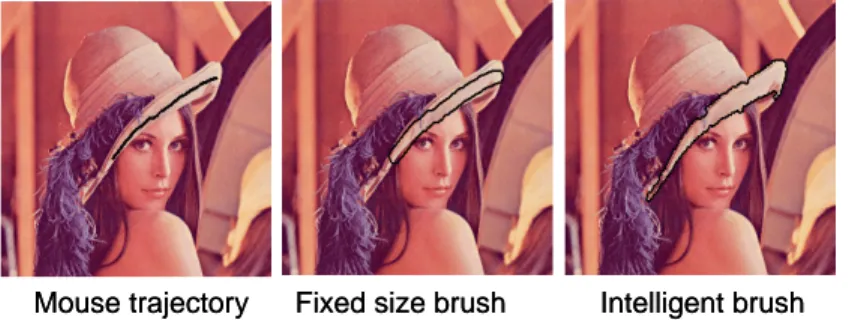
Intelligent brush An intelligent brush segments an image by ”painting” it: it …rst selects a zone of interest by painting. Contrary to conventional brushes, the brush adapts its shape to the contours of the image. The shape of the brush is given by the region of the hierarchy containing the cursor. Moving from one place to another changes the shape of the brush, when one goes from one tile of a partition to its neighboring tile. Going up and down the hierarchy modi…es the shape of the brush. In …g.1, on the left, one shows the trajectory of the brush ; in the centre, the result of a …xed size brush, and on the right the result of a self-adapting brush following the hierarchy. This self adapting brush is nothing by the dilation rby a ball associated to the hierarchy, centered at the
position of the mouse and of a radius, also easily modi…ed through the mouse. This method has been used with success in a package for interactive segmention of organs in 3D medical images.
Mouse trajectory Fixed size brush Intelligent brush Mouse trajectory Fixed size brush Intelligent brush
Figure 1: Comparison of the drawing with a …xed size brush and a self adaptive brush.
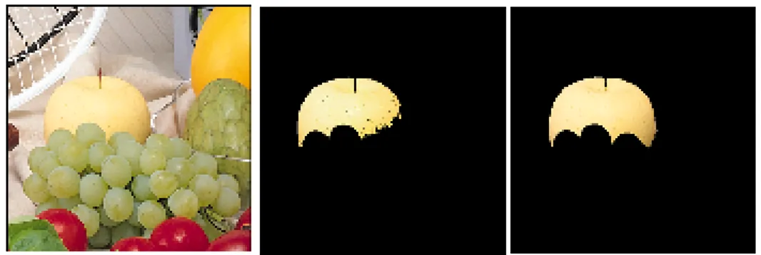
Figure 2: Left: initial image Center: result of the magic wand
Right ; smallest region of the hierarchy containing the magic wand.
Magic wand The magic wand in a conventional computer graphics tool-box consists in extracting the region which touches the position of the mouse and whose colour lies within some prede…ned limits from the coulour at the mouse position. The next step consists in replacing this set by the smallest set of the hierarchy which contains it. This operation is a closing, described by Ch. Ronse in [4]. The result is shown in …g.2
3
The lattice of hierarchies
It is often interesting to combine several hierarchies, in order to combine vari-ous criteria or merge the information obtained from diverse sources (colour or multispectral images for instance). We …rst de…ne an order relation between hierarchies which structures them into a complete lattice.
3.0.6 Order relation
Complete hierarchies Let A and B be two strati…ed hierarchies, with their associated half-distances : Aand B: The following relation de…nes an order relation between the hierarchies: B < A , 8p; q 2 E A(p; q) B(p; q)
It follows that 8p 2 E : BallB(p; ) BallA(p; )
With this order relation the hierarchies of P(E) form a complete lattice. The maximal element is the hierarchy having E as only element and the smallest hierarchy contains only singletons fxg :
Partial hierarchies This order also holds for partial hierarchies. Let A and B be two strati…ed partial hierarchies, with their associated half-distances : A and B: The following relation de…nes an order relation between the hierarchies: B < A , 8p; q 2 E A(p; q) B(p; q) : For each p =2 supp(A) : A(p; p) =
L; which implies that B(p; p) = L; indicating that supp(A) supp(B); or equivalently supp(B) supp(A)
The smallest partial hierarchy contains only aliens, i.e. points p verifying 8q 2 E ; (p; q) = L:
Particular case of partitions Let A and B be two partitions, with their associated binary half-distances : dAand dB: The partition B is …ner than the partition A i¤ 8p; q 2 E dA(p; q) dB(p; q)
It follows that 8p 2 E : BallB(p; ) BallA(p; )
But the balls of a partition BallB(p; ) are the tiles of this partition. Hence the tiles of the …ner partition B are included in the tiles of the coarser partition A which is coherent with the usual de…nition of the order between partitions. 3.0.7 In…mum of two hierarchies
Complete hierarchies The in…mum of two hierarchies A and B is written A ^ B and is de…ned by its ultrametric half-distance dA^B= dA_ dB. It is easy
to check that it is indeed a half-distance. It is symmtrical and half-positive. Let us check the ultrametric inequality:
(dA_ dB) (p; r)_(dA_ dB) (r; q) = (dA(p; r) _ dA(r; q))_(dB(p; r) _ dB(r; q)) > (dA(p; q) _ dB(p; q)) = dA_ dB(p; q)
Its balls are de…ned by : 8p 2 E : BallA^B(p; ) = BallA(p; ) ^ BallB(p; )
Partial hierarchies If A and B are partial hierarchies, their supremum is de…ned as for the hierarchies. The aliens of a partial hierarchy X are charac-terized by 8p; q 2 E : (p; q) = L: Hence the aliens of A ^ B are the union of the aliens of A and of B, i.e. supp(A ^ B)=supp(A)_supp(B) or equivalently supp(A ^ B) = supp(A)^ supp(B):
3.0.8 In…mum of two hierarchies
The subdominant ultrametric half-distance The supremum of two hier-archies A and B is written A _ B and is the smallest hierarchy larger than A and B.
As dA^ dB is not an ultrametric distance, we chose for dA_B the largest ultrametric distance which is lower than dA^ dB: This distance exists: the set of ultrametric distances lower than dA^ dB is not empty, as the distance 0 is ultrametric ; furthermore, this family is closed by supremum, hence it has a largest element. Let us construct it.
Consider a series of points (x0; x1; ; xn): As dA_Bshould be an
ultramet-ric distance, we have for any path x0; x1; :::; xn
dA_B((x0; xn) dA_B(x0; x1) _ dA_B(x1; x2) _ _ dA_B(xn 1; xn):
But for each pair of points xi; xi+1we have dA_B(xi; xi+1) [dA^ dB] (xi; xi+1):
Hence dA_B(x0; xn) [dA^ dB] (x0; x1)_[dA^ dB] (x1; x2)_ _d [dA^ dB] (xn 1; xn):
There exists a chain along which the expression on the right becomes minimal and is equal to the maximal value taken by [dA^ dB] on two successive points of
the chain. This maximal value is called sup section of the chain for dA^ dB: For this reason, the chain itself is called chain of minimal sup-section. This valua-tion being an ultrametric ecart necessarily is the largest ultrametric ecart below dA^ dB: Let us verify the ultrametric inequality.
For p; q; r 2 E there exists a chain between p and q along which [dA^ dB] (p; q)
takes its value and another chain between q and r along which [dA^ dB] (q; r) takes its value. The concatenation of both chains forms a chain between p and q which is not necessarily the chain of lowest sup-section between them, hence:
[dA^ dB] (p; r) [dA^ dB] (p; q) _ [dA^ dB] (q; r):
We write ^dA^ dBfor the subdominant ultrametric associated to dA^ dB:
Partial hierarchies If A and B are partial hierarchies, their in…mum is de-…ned as for the hierarchies. The aliens of a partial hierarchy X are characterized by 8p; q 2 E : (p; q) = L: Hence the chains characterizing the subdominant ul-trametric distance associated to A _ B avoid the supports supp(A) and supp(B). Geometrical interpretation Suppose that (x0; x1; ; xn) is the chain for
which ^dA^ dB(x0; xn) = [dA^ dB] (x0; x1)_[dA^ dB] (x1; x2)_ _[dA^ dB] (xn 1; xn)
is minimal with a value : Then [dA^ dB] (xi; xi+1) means that the ball
BallA(xi; ) or the ball BallB(xi; ) contains the point xi+1: If it is BallA(xi; );
then xi+1 also is center of this ball. Hence a series of points xk; xk+1; xk+2;
all belong to the same ball BallA(xi; ), they are all centers of this ball and it
is possible to keep only one of them and suppress all others from the list. Like that we get a path where the …rsts two points x0; x1 belong to one of the balls,
say BallA(x0; ); the couple x1; x2 belong to the other BallB(x2; ); and so on.
The successive ovelapping pairs of points belong alternatively to balls BallAor BallB:
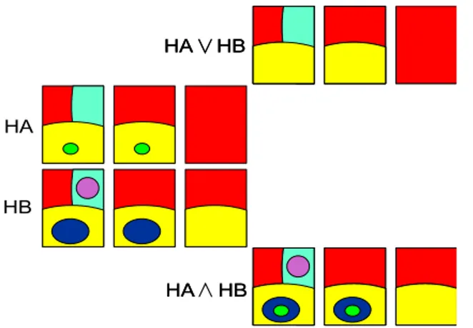
The necessity of chaining blocks for obtaining suprema of partitions is well known [6] ; Ronse has con…rmed that it is still the case for partial partitions [4]. Illustration If A , B and A _ B are the partitions obtained by taking the balls of radius in each of the three hierarchies, then the boundaries of A _ B are all boundaries existing in both A and B . The in…mum and supremum of two hierarchies are illustrated in …g.3
3.1
Lexicographic fusion of strati…ed hierarchies
Let A and B be two strati…ed hierarchies, with their associated distances dA
and dB: In some cases, one of the hierarchies correctly represents the image to segment, but with a too small number of nested partitions. One desires to enrich the current ranking of regions as given by A; by introducing some intermediate levels in the hierarchy. The solution is to combine the hierarchy A with another hierarchy B in a lexicographic order.
One produces the lexicographic hierarchy Lex(A; B) by de…ning its ultra-metric distance ; it is the largest ultraultra-metric distance below the lexicographic
Figure 3: Two hierarchies HA and HB and their derived supremum and in…mum
Initial Image H component V component Infimum Initial Image H component V component Infimum
Figure 4: Supremum of two hierarchies.
distance dA;B classically de…ned by dA;B(C; D) > dA;B(K; L) ,
dA(C; D) > dA(K; L) or
dA(C; D) = dA(K; L) and dB(C; D) > dB(K; L)
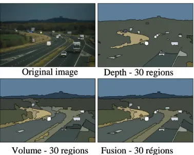
Fig.5 present two hierarchies HA and HB and the derived lexicographic hierarchies Lex(A; B) and Lex(B; A): Fig. shows an image which is di¢ cult to segment as it contains small contrasted objects, the cars and the landscape and road which are much larger and less contrasted. Two separate segmentation have been performed. The …rst based on the contrast segments the cars ; the second, based on the "volume" (area of the regions multiplied by the contrast) segments the landscape. The hierarchy of both these segmentations has been thresholded so as to show 30 regions. The lexicographic fusion of both seg-mentations Lex(Depth; V olume); also thresholded at 30 regions o¤ers a nice composition of both segmentations.
HA
HB
Lex(HA,HB)
Lex(HB,HA)
Figure 5: Two hierarchies HA and HB and their derived lexicographic combi-nations.
Depth - 30 regions
Fusion - 30 régions
Original image
Volume - 30 regions
Depth - 30 regions
Fusion - 30 régions
Original image
Volume - 30 regions
4
Connected operators
5
Adjunctions on hierarchies
Given a point O serving as origin, a structuring element B is a family of transla-tionsS n !Ox j x 2 Bo: A set X of P(E) may then be eroded and dilated by this structuring element : the erosion X B = V
x2B
XOx! and the dilation X B = W
x2B
XxO!: As one uses for one operator the vectors Ox and for the other the! vectors Ox =! xO; both operators form an adjunction: for any X; Y 2 P(E);! we have X B < Y , X < Y B:
A hierarchy X 2 X (E) is a collection of sets Xi 2 P(E): Through the translation by a vector !t ; these sets Xi
!t form a new hierarcy X!t: If is the
ultrametric ecart associated to X , the ultrametric ecart associated to X!t will be written !t:
As the hierarchies form a complete lattice X (E), we may use the same mechanism for constructing an erosion and a dilation on hierarchies. We de…ne two operators operating on a hierarchy X . For showing that the …rst X B =
V
x2BX !
Ox is an erosion and the second X B =
W
x2BX !
xO a dilation, we have to
show that they form an adjunction.
We have to prove that for any two hierarchies X ; Y 2 X (E) : X B < Y , X < Y B:
We will prove the adjunction through the half distance associated to the hierarchies X and Y.
We have the following correspondances between the hierarchies and the ul-trametric ecarts : X $ Y $ Y B = V x2BY ! Ox $ W x2B ! Ox X B = W x2BX ! xO $ ^ V x2B ! xO X B < Y , X < Y B $ ^V x2B ! xO> , > W x2B ! Ox
Let us now prove the adjunction.
For two arbitrary ultrametric ecarts and : X < Y B , > W
x2B ! Ox, 8x 2 B : > ! Ox, 8x 2 B : xO!> , V x2B ! xO> Remains to establish : V x2B ! xO> , ^ V x2B ! xO> :
Initial partition
Eroded partition
Figure 7: Erosion of a partition^ V x2B ! xO> ) V x2B ! xO> since ^ V x2B !
xOis the largest ultrametric ecart
below V x2B ! xO Suppose now V x2B !
xO> : Since is an ultrametric ecart below
V
x2B ! xO;
it is smaller or equal to the largest ultrametric ecart below V
x2B ! xO; that is V^ x2B ! xO:
This completes the proof : X < Y B , > W x2B ! Ox , V x2B ! xO> , ^ V x2B ! xO> , X B < Y
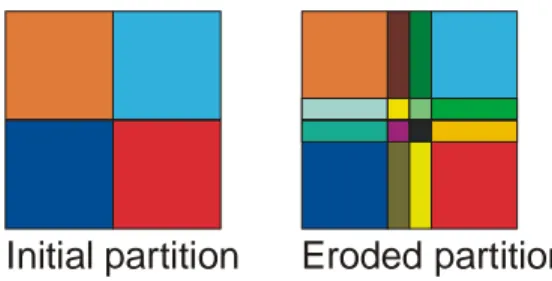
The erosion of a partition by a square structuring element (8 connexity) is illustrated in …g.7
Remark 11 The adjunction de…ned for hierarchies is de…ned in a similar fash-ion for a partial hierarchy.
5.1
Decomposition and recomposition of hierarchies
5.1.1 Thresholding
Consider a hierarchy X with its associated ultrametric ecart : By thresholding the ultrametric at level one obtains a binary ultrametric ecart :
T ( ) = 1 if > 0 if
T ( ) characterizes a partition.
The hierarchy can be recovered from its thresholds by =W T ( ): Remark 12 If X is a partial hierarchy, then T ( ) is a partial partition 5.1.2 Reconstructing a hierarchy
Inf-generation Consider a hierarchyX , union of a family (Ai) of P(E). If
a set Ai belongs to X , then we construct a partition by adding to Ai its
complement. We have de…ned this operator earlier Backg(Ai) = Ai [ Ai to
which we associate the binary ultrametric ecart i:
The ultrametric ecart associated to X is sup-generated and equal to W
i
st(Ai) i and the hierarchy is inf-generated by the partitions Backg(Ai)
weighted by their strati…cation level.
This decomposition helps understanding how the erosion of ultrametric hier-archies work. To X B is associated B = W
i
st(Ai) i B =W i
[st(Ai) i]
B
For each set Ai; the partition Ai[ Ai is eroded, that is the new partition
Ai[ (Ai=Ai B) [ Ai=Ai B [ Ai is created. This partition keeps the same
strati…cation level as Ai itself. This new collection of partitions creates the
eroded hierarchy.
Remark 13 In the particular case of a partition, the sets forming this partition are eroded, and the space left by the erosion is …lled by the intersection of all partial partitions (Ai=Ai B) [ Ai=Ai B . The result is illustrated by …g.7.
This di¤ ers from the de…nition given by J.Serra in [7], where he …lled the spaces left empty by singletons.
Sup-generation Consider a hierarchy X , union of a family (Ai) of P(E). We
associate to the set Ai the following half-distance i:
For any p; q 2 Ai : i(p; q) = st(Ai). For p =2 Ai; and any q we have i(p; q) = L: We have thus associated to the set Ai a partial partition equal to
Ai on Ai; with a strati…cation level st(Ai) and containing only aliens on Ai:
The half-distance is then inf-generated and equal to V
i
i, corresponding
to the sup-generation from the partial hierarchies cAi associated to the i:
This decomposition helps understanding how the dilation of ultrametric hi-erarchies work. To X B =W
i
c
Ai B is associated the half-distance
^ V
i
i B
5.2
Illustration
We illustrate the erosion and the opening of a one dimensional hierarchy, …rst by a structuring element reduced to two pixels, then by a structuring element made of three pixels. In the …rst case, the erosion and the dilation have to use the structuring element for the erosion and its transposed version for the dilation.
5.2.1 Erosion and opening by a pair of 2 pixels. 3 2 1 4 2 3 2 1 4 2 3 2 1 4 2 3 2 1 4 2 3 2 1 4 2 3 2 4 2 1 3 2 4 2 Image de départ Translation droite Erosion Translation gauche Ouvert
Erosion and opening by a pair of pixels: intermediate steps
3 2 1 4 2
3 2 1 4 2 1
Ouverture par un bi-point Image de départ
Dendrogram of an initial image and its opening by a segment of 2 points. 5.2.2 Erosion and opening by a centered segment of 3 pixels.
3 2 1 4 2 3 2 1 4 2 3 2 1 4 2 3 3 3 2 2 2 4 4 4 2 2 2 3 2 2 2 2 2 4 2 2 2 3 3 3 2 2 2 4 4 4 2 2 2 3 3 3 2 2 2 4 4 4 2 2 2 3 2 1 4 2 Image de départ Translation droite Translation gauche Erosion Translation droite Translation gauche Ouvert Image de départ
3 2 1 4 2
3 2 2 2 2 2 4 2 2 2
Ouverture par 3 points Image de départ
Dendrogram of an initial image and its opening by a segment of 3 points.
5.3
Examples of hierarchies
Hierarchies associated to a dissimilarity index A series of nested parti-tions (Xi) ; and hence a hierarchy, may easily be generated from an initial …ne
partition X0 = [Ri, i = 1; : : : ; n on which a dissimilarity index is de…ned
between a subset G of all couples of tiles. For a couple of tiles which do not belong to G; we de…ne a dissimilarity equal to 1:
If we now take the union of all tiles of X0with a dissimilarity index below a
given threshold ; we obtain a coarser partition with a strati…cation index equal to . For increasing values of we obtain a series of nested partitions, forming a hierarchy A. The ultrametric distance d associated to this hierarchy is precisely the the subdominant ultrametric distance associated to , that is the largest ultrametric distance below (see below the supremum of two hierarchies, where the subdominant ultrametric distance also appears) For two tiles A and B of X0; the subdominant ultrametric distance will be the lowest level for which A
and B belong to the same tile (if it does not happen, their distance is 1) Case of the watershed tesselation If the tessellation is the result of the watershed construction on a gradient image, the dissimilarity measure can be de…ned as the altitude of the pass point separating two adjacent regions. The ultrametric half distance between two minima is then the "‡ooding distance" : the ‡ooding distance between two points p and q is the altitude of the lowest ‡ooding for which p and q both belong to a common lake.
Other possible measures are color distances, various measures of local con-trast, or even motion or texture dissimilarity between adjacent catchment basins.
6
Connectivity and taxonomy classes
The notion of a connected set in E is well de…ned if E is a topological space. In [6], Serra generalized this concept by the introduction of a connectivity class. Connectivity classes de…ne the subsets of E which are connected. Hence they help decomposing every set X 2 P(E) into its connected components. Connec-tivity classes have been extensively studied by Serra and Ronse ([8],[4]).
We extend here the notion of connectivity classes and de…ne taxonomy classes. We present in parallel the notions related to partitions and to hierar-chies. For our presentation of the binary case, we largely follow Henk Heijmans, who gives a clear presentation of the developments linked to connectivity in [2].
6.1
Connectivity and taxonomy classes
6.1.1 General de…nition Connectivity classes
De…nition 14 Let E be an arbitrary nonempty set. A family C P(E) is called a connectivity class if it satis…es
(C1) ? 2 C and fxg 2 C for x 2 E (C2) if Ci2 C and T i2I Ci6= ?; then S i2I Ci 2 C
Alternatively, we say that C de…nes a connectivity on E: An element of C is called a connected set. This de…nition is "generative" : larger connected sets are generated from elementary ones with a non empty intersection.
Taxonomy classes
De…nition 15 Let E be an arbitrary nonempty set. H = (Hi)i2I is called a
taxonomy class if Hi P(E) satisfy
(H1) for i 2 I : ? 2 Hi and fxg 2 Hi for x 2 E
(H2) Hi Hj for j > i (H3) if for i 2 J I; k 2: Hk 2 H i and T k2K Hk 6= ?; then S k2K Hk 2 H max(J )
H is called a taxonomy, each Hi a taxonomy class and Hk 2 Hi a taxon of
level i:
This de…nition is compatible with the de…nition of a connectivity class, in the case where H contains only one element : if J contains only one index l; then Hlis a connectivity class, as the axioms (C1) and (C2) are veri…ed. This shows
that any taxonomy class is a series of nested connectivity classes. Inversely, it is obvious that a series of nested connectivity classes is a taxonomy.
6.1.2 Adjacency relations Connectivity classes
An important subclass of connectivity classes is based on adjacency.
De…nition 16 A binary relation on E E is called an adjacency relation if it is re‡exive (x x for every x) and symmetric (x y i¤ y x).
Given an adjacency relation on E E; we call x0; x1; :::; xn a path between
x = x0 x :::: xn = y: De…ne C P(E) as the collection of all C 2 E
such that any two points in C can be connected by a path that lies entirely in C:
Proposition 17 If is an adjacency relation on E E, then C is a connec-tivity class.
Proof. (C1) is obvious. If Ci 2 C and z 2 T i2I
Ci; we have to show that any
two points x; y in S
i2I
Ci can be connected by a path that lies entirely in S i2I
Ci:
There exists two indices in I such that x 2 Ci1 and x 2 Ci2: There exists a path
linking x with z in Ci1 and a path linking z with y in Ci2: The path between x
and y is obtained by concatenating both paths.
De…nition 18 C is a strong connectivity class if there exists an adjacency re-lation on E E such that C~ and E is connected. We say that E possesses
a strong connectivity. Taxonomy classes
For de…ning a taxonomy class we need a series of nested adjacency relations (the adjacency between a cat and another cat, or between a cat and a tiger, or a tiger and a mammal cannot be the same).
De…nition 19 A family (ei)i2I of adjacency relations is nested if x ei y implies
x ej y for j > i:
To each adjacency relation ei we associate its connectivity class Cei
Proposition 20 If the family (ei)i2I of adjacency relations is nested, then the
family H = (Cei)i2I is a taxonomy class.
Proof. (H1) is trivially veri…ed. (H2) is veri…ed as x ei y implies x ej y for j > i; hence CT ei Cej: Let us prove (H3). Suppose that for i 2 J : Hk 2 Ceiand k2K
Hk 6= ?: If l = max(J) is the maximal index of J, we have Hk 2 C ei
Cel: And as Cel is a connectivity class,
T k2K Hk 6= ? implies S k2K Hk 2 C el: Example
Consider a grey tone image f de…ned on a grid with a neighborhood relation. We de…ne the adjacency relation p ei q by the following conditions:
p and q neighbors on the grid jfp fqj i
For the value i; the connected components are the lambda-‡at zones of slope i: For increasing values of i; this slope increases and so do the lambda ‡at zones.
6.1.3 Connectivity openings Connectivity classes
Serra in [6] has shown that any connected class C is equivalent with the datum of a connected opening, de…ned through its invariance domain. If Cx denotes
the subclass of C 2 C that contains a given point ; Cx= fC : x 2 C Cg
then the union of each non-empty family of sets of Cx; all containing x still
belongs to Cx; because of (C2). Hence Inv( x) = Cx[ f?g is the invariant set
of an opening x; called connected opening of origin x: Its expression is
x(X) =
S
fC : x 2 C C and C Xg Since any x 2 E belongs to a connected set of C, we have
C = S
x2E
Inv( x)
Proposition 21 Assume that C is a connectivity on E, then the following con-ditions are satis…ed:
(O1) every x is an opening (O2) x(fxg) = fxg
(O3) x(X) \ y(X) = ? or x(X) = y(X) (O4) x =2 X ) x(X) = ?
Conversely if x; x 2 E; is a family of operators satisfying (O1)-(O4) then C = S
x2E
Inv( x) de…nes a connectivity.
The principal interest of connection openings lies in the following corollary of [6]
Corollary 22 Openings x partition any X E into the smallest possible number of components belonging to the class C.
Given a set X E; every connected component x(X) of X is called a grain of X: The next result ([2]) says that every connected subset of X is contained within some grain of X
Proposition 23 Given a connectivity on E and a set X E: If C X is a connected set, then C is contained within some grain of X:
Another useful property ([6]), shows that x plays no particular role in x(X): Corollary 24 For all x; y 2 E and all X E we have
y 2 x(X) , x(X) = x(X) and in particular y 2 x(X) , x 2 y(X)
De…nition 25 Given a space E; a function P : E ! P (E) is called a partition of E if
(i) x 2 P (x); x 2 E
(ii) P (x) = P (y) or P (x) \ P (y) = ?; for x; y 2 E
If E is endowed with a connectivity C and if P (x) 2 C for every x 2 E; then we say that the partition P is connected.
Given a connective class, every binary image (i.e.set) X E can be associ-ated with a connected partition P (X) where the zones of P (X) are the grains of X and Xc: The zone of P (X) containing a point p is :
P (X)(p) = p(X) if p 2 X
p(Xc) if p =2 X
Corollary 26 For all x; y 2 E and all X E we have
y 2 P (X)(x) , P (X)(x) = P (X)(y) and in particular y 2 P (X)(x) , x 2 P (X)(y)
Proof. If x 2 X, y 2 P (X)(x) = x(X) ) P (X)(x) = x(X) = y(X) =
P (X)(y) and x 2 y(X) = P (X)(y)
If x 2 Xc; the proof is similar, replacing X by Xc
Corollary 27 For all x; y 2 E and all X E we have y =2 P (X)(x) , P (X)(x) \ P (X)(y) = ?
Proof. If x 2 X and y =2 X; or vice-versa, then the implication is obvious. Consider the case where x; y both belong to X or both belong to Xc: Sup-pose that there exists a point z 2 P (X)(x) \ P (X)(y) ; this would imply that P (X)(x) = P (X)(z) = P (X)(y) which contradicts the hypothesis
Connected operators
De…nition 28 An operator on P(E) is connected if the partition P ( (X)) is coarser than P (X) for every set X E
Taxonomy classes
Consider a taxonomy class H = (Hi)i2I. Each Hi is a connectivity class to
which is associated a connection opening i x:
Hi also segments every binary image (i.e.set) X E into a connected
par-tition Pi(X): The grains of this partition are the sets Pi(X)(x); for x 2 E.
Lemma 29 For j > i; we have Pi(X)(x) Pi(X)(x) for x 2 E
Proof. ix(X) =
S
fC : x 2 C Hi and C Xg and Hi Hj for j > i; it
follows that i
x(X) jx(X) and Pi(X)(x) Pj(X)(x) for j > i:
Proposition 30 The family (Pi(X)(x))i2I;x2E[ f?g forms a hierarchy. We
Proof. We have to verify that both the intersection axiom and union axiom are satis…ed
(Intersection axiom)
Consider two sets of the hierarchy Pi(X)(q) and Pj(X)(p) for i j
a) q 2 Pj(X)(p) : then Pj(X)(p) Pj(X)(q) and since Pi(X)(q) Pj(X)(q);
the result Pi(X)(q) Pj(X)(p) is proved
b) q =2 Pj(X)(p) then Pj(X)(p) \ Pj(X)(q) = ?: Since Pi(X)(q) Pj(X)(q)
we also have Pi(X)(p) \ Pj(X)(q) = ?
(union axiom)
Consider a set A = Pj(X)(p) of the hierarchy. For a point q 2 Pj(X)(p) we
have also Pj(X)(q) = Pj(X)(p): Since Pi(X)(q) Pj(X)(q) for i j; it shows
that Pj(X)(q) Pj(X)(p)
Hence Pj(X)(p) = S q2A;i<j
Pi(X)(q) is indeed the union of the elements of the
hierarchy it contains. The family (Pi(X)(x))
i2I;x2E forming a hierarchy, we may apply to it all
results we have established in the …rst part of the paper, in particular we may associate to it an ultrametric half-distance (X)
Connected operators
De…nition 31 An operator on P(E) is connected if the hierarchy XH( (X)) is coarser than XH(X) for every set X E
This means that the identity operator from the half-metric space E with the half distance H(X) into the half-metric space E with the half distance
H( (X)) is Lipschitz, as for any two points p; q 2 E; we have H( (X))(p; q) H(X)(p; q)
7
Conclusion
We may now give a summary of the results, which are all linked to the properties of the ultrametric half distances.:
each point is centre of a ball
two balls with the same radius are either disjoint or identical
two balls with a di¤erent radius are either disjoint or one is included in the other
Finally, rather than starting with a hierarchy and de…ning an ultrametric half-distance, we rather start with an ultrametric half-distance which helps de-riving all other concepts:
two taxons A and B have an empty intersection or they form a taxon with a diameter equal to diam(A) _ diam(B)
the connected opening : i
p(X) = ix(X) =
S
fC : x 2 C Hi and C Xg
The grain at level i of the hierarchy associated to X : Pi(X)(p) = i
p(X) if p 2 X i
p(Xc) if p =2 X
Adjacence relations : the ultrametric half distance may be de…ned if one knows the distance (p; q) for a collection of pairs of points (p; q). From them it is possible to construct all taxonomy classes and obtain the hierarchy by adding the singletons and the empty set.
References
[1] J. P. Benzécri. L’analyse des données 1. La taxinomie, chapter 3, pages 119–153. Dunod, 1973.
[2] H. J. A. M. Heijmans. Connected morphological operators for binary images. Computer Vision and Image Understanding, 73(1):99 –120, 1999.
[3] F. Meyer. An overview of morphological segmentation. International Journal of Pattern Recognition and Arti…cial Intelligence, 17(7):1089–1118, 2001. [4] C. Ronse. Adjunctions on the lattices of partitions and of partial partitions.
Appl. Algebra Eng. Commun. Comput., 21(5):343–396, 2010.
[5] L. Schwartz. Analyse : topologie générale et analyse fonctionnelle, chapter 3, pages 233–240. Hermann, 2008.
[6] J. Serra, editor. Image Analysis and Mathematical Morphology. II: Theoret-ical Advances. Academic Press, London, 1988.
[7] J. Serra. Morphological operators for the segmentation of colour images. In M. S. M. Bilodeau, F. Meyer, editor, Space, structure, and randomness. Contributions in honor of Georges Matheron in the …elds of geostatistics, random sets, and mathematical morphology., pages 223–255. Lecture Notes in Statistics 183. New York, NY: Springer. xviii, 395 p., 2005.
[8] J. Serra. A lattice approach to image segmentation. J. Math. Imaging Vis., 24:83–130, January 2006.
[9] M. F. Zanoguera, B. Marcotegui, and F. Meyer. An interactive colour image segmentation system. In Wiamis’99 : Workshop on Image Analysis for Mul-timedia Interactive Services, pages 137–141. Heinrich-Hertz Institut Berlin, 1999.