One-Dimensional Openings, Granulometries and Component Trees in O(1) Per Pixel

HAL Id: hal-00879627

https://hal.archives-ouvertes.fr/hal-00879627

Submitted on 4 Nov 2013

HAL is a multi-disciplinary open access

archive for the deposit and dissemination of

sci-entific research documents, whether they are

pub-lished or not. The documents may come from

teaching and research institutions in France or

abroad, or from public or private research centers.

L’archive ouverte pluridisciplinaire HAL, est

destinée au dépôt et à la diffusion de documents

scientifiques de niveau recherche, publiés ou non,

émanant des établissements d’enseignement et de

recherche français ou étrangers, des laboratoires

publics ou privés.

Component Trees in O(1) Per Pixel

Vincent Morard, Petr Dokládal, Etienne Decencière

To cite this version:

Vincent Morard, Petr Dokládal, Etienne Decencière. One-Dimensional Openings, Granulometries and

Component Trees in O(1) Per Pixel. IEEE Journal of Selected Topics in Signal Processing, IEEE,

2012, 6 (7), pp.840-848. �10.1109/JSTSP.2012.2201694�. �hal-00879627�

One-dimensional openings, granulometries and

component trees in

O(1) per pixel

Vincent Morard, Petr Dokl ´adal and Etienne Decenci `ere

F

Abstract—We introduce a new, efficient and adaptable algorithm to

compute openings, granulometries and the component tree for one-dimensional (1-D) signals. The algorithm requires only one scan of the signal, runs in place in O(1) per pixel, and supports any scalar data precision (integer or floating-point data).

The algorithm is applied to two-dimensional images along straight lines, in arbitrary orientations. Oriented size distributions can thus be efficiently computed, and textures characterised.

Extensive benchmarks are reported. They show that the proposed algorithm allows computing 1-D openings faster than existing algorithms for data precisions higher than 8 bits, and remains competitive with respect to the algorithm proposed by Van Droogenbroeck when dealing with 8-bit images. When computing granulometries, the new algorithm runs faster than any other method of the state of the art. Moreover, it allows efficient computation of 1-D component trees.

Index Terms—Algorithms, Mathematical Morphology, Opening,

Granu-lometry, Component Tree, Oriented size distribution, Filtering.

1

I

In the framework of mathematical morphology [1], [2], any anti-extensive, increasing and idempotent operator is an algebraic opening. This fundamental family of operators is often based on a structuring element (SE) probing the image at different places; in this case, it is called a morphological opening. Using a segment as structuring element is useful to detect straight structures, or to find the local orientation of thin objects. Indeed, many practical applications involve a directional analy-sis (Material characterisation, crack detection, biological applications [3], [4]).

In this paper, the presentation is limited to openings, but all results can be directly applied to their dual operators, the closings.

Openings can be used to build granulometries [5]– [7]. This tool was initially introduced to study porous media [5] and it can be seen as a sieving process. Given some powder composed of particles of different radii, sieves of decreasing size are used to perform a size analysis of these particles, by measuring the quantity of powder left in each sieve. Many image processing applications involve granulometries, size distribution, image segmentations or texture characterisations [7]–[9].

The author are with MINES ParisTech, CMM - Centre of Mathematical Morphology, 35, rue St. Honor´e, 77305-Fontainebleau-Cedex, France.

Multi-scale image analysis can also be based on the component tree (or max-tree). Introduced by Salembier [10], it captures some essential features of an image. This tree structure is used in many applications including im-age filtering, imim-age segmentation, video segmentation, and image compression [11]–[13]. It is also at the basis of the topological watershed [14].

All these operators are time consuming with naive implementations and many authors have developed fast and efficient algorithms to deal with this issue.

For morphological openings (i.e. openings using a structuring element), Pecht [15] defined in 1985 a log-arithmic decomposition of the structuring element. This decomposition removes most of the redundancy. Later, Van Herk [16] on the one side, and Gil and Werman [17] on the other side, reduced the complexity to a constant per pixel. This algorithm, called hereafter HGW, is independent of the size of the structuring element for the computation of one-dimensional (1-D) erosions and dilations. Later, Clienti et al. improved HGW algorithm by removing the backward scanning to ensure a low latency [18]. Then, algorithms have also been proposed to compute openings in only one pass of the entire image, without computing successively the erosion and the dilation. Van Droogenbroeck and Buckley developed an algorithm based on so-called anchors [19]. The al-gorithm uses image histogram. It is extremely efficient on 8-bit data, but its performance decreases with higher precision data. Later, Bartovsk ´y et al. [20] worked on a new streaming algorithm with a minimal latency and a low memory requirement.

For granulometries, a straightforward approach con-sists in computing a set of openings of different sizes, and measuring the residues between two successive openings. This is a very computationally intensive task. Vincent proposed an efficient algorithm based on the re-cursive analysis of the regional maxima of the signal [21]. This algorithm is faster by several orders of magnitude over the naive implementation and highly contributed to the diffusion of this tool in the image processing community.

In the literature, many authors have worked on the 1-D component tree. Among them, Najman and Couprie [22] built an algorithm in quasi linear time and more recently, Menotti et al. [23] downed the complexity to a

constant per pixel.

In this never-ending struggle for faster algorithms, we propose a new algorithm, which competes favourably with existing ones when computing openings, and also allows computing granulometries and component trees - all this in one dimension. It can also deal with various data accuracy (it is not limited to integers). In fact, in can be applied to any kind of data, as long as the values belong to an ordered group. A first, shorter, description of this work was previously presented by the authors [24].

This paper is organised as follows: section 2 recalls the basic notions on attribute openings and granulome-tries, whereas section 3 describes the algorithm to build granulometries, openings and the component tree for 1-D signals. Then, section 4 applies this algorithm to two-dimensional (2-D) images, and finally, sections 5 and 6 study the complexity and the timings through a comparison with the state-of-the-art.

2

B

In this section, the definitions of one-dimensional at-tribute openings and size distributions are recalled. Moreover, it is explained how to apply them to two-dimensional images.

2.1 Attribute openings

Let X : D → {0; 1} be a binary signal, where D is an interval of Z such as [1, N ]. We define {Xi} as the

collection of connected components (CC) of X and Xi

the ith _{element of this set. Note that in 1-D these CCs}

are intervals of Z. We wish to keep or delete these CCs according to an attribute associated to a criterion χ (e.g. “the length is larger than λ”). Formally, χ is a function mapping the set of CCs of D into {f alse, true}, which allows to define a function ψ:

ψχ(Xi) =

(

Xi if χ(Xi)is true

∅ otherwise, (1) for all CCs Xiincluded in D. Based on this function, the

corresponding attribute opening can be introduced for all binary signals X:

γχ(X) =

[

Xi∈{Xi}

ψχ(Xi). (2)

Hereafter, the chosen attribute will be the length of the CC. The resulting criterion will be “is longer than or equal to λ”, and the corresponding opening will be denoted γλ. However, other attributes can be used, for

example, whether the CC contains a point from another set (which would allow building openings by reconstruc-tion).

From now on, consider f : D → V , with V equal to Z or R. Let Xh _{= {x|f (x) ≥ h} be the set obtained}

by thresholding f at level h. Recall that an opening is

(a) Input (b) γα χ (c) ∨γχ 0 90 180 45 135 (d) ζχ

Fig. 1. Application of linear openings with the criterion χ : “length ≥ 21 pixels”. (a) initial image with a zoom on a part of the image. (b) oriented filtering: only straight structures longer than 21 pixels oriented at α = 70 degrees are kept. (c) preservation of all linear structures longer than 21 pixels. (d) local orientation in false colours.

an increasing, anti-extensive and idempotent operator. Thanks to the increasingness, the opening commutes with the thresholding. Thence, the extension of openings to grey level images is direct:

γχ(f ) = ∨{h ∈ V | x ∈ γχ(Xh(f ))}. (3)

We will introduce in section 3 an efficient algorithm to compute these linear openings. In order to apply it to two-dimensional images, we can consider a given orien-tation α, and decompose the image into one-dimensional signals, following this orientation (see section 4 for de-tails). Therefore, we get a directional opening written γα

χ.

Further directional operators can be built with these lin-ear openings. The first one is ∨γχ(f ), which is computed

by taking the supremum of the attribute openings in all orientations:

∨γχ(f ) =

_

α∈[0,180[

γαχ(f ) (4)

The second one, ζχ(f ), can extract the local orientation

of the structures by storing, on each pixel, the angle of the opening producing the highest grey value:

ζχ(f ) = argsup α∈[0,180[

γ_χα(f ). (5) Fig. 1 illustrates the results of these operators on a fingerprint image.

2.2 Size distribution

A size distribution, also called granulometry, is built from openings. As proposed by Matheron [5], a family (γν)ν≥0 of openings is a granulometry if, and only if:

∀ν ≥ 0, ∀µ ≥ 0, ν ≥ µ ⇒ γν ≤ γµ. (6)

Later, Maragos introduced the pattern spectrum [7]: (PS(f ))(ν) =−d(Meas(γν(f )))

with Meas(), a given additive measure. In the discrete case, the differential function is replaced by a subtraction between two consecutive openings. By analysing these residues, we get the measure of all the structures that have been removed from the image at this scale. There-fore, the discrete pattern spectrum is defined as follows: (PS(f ))(ν) = Meas(γν(f ) − γν−1(f )), ν > 0. (8)

Fig. 2 explains how a 1-D signal is decomposed. The pattern spectrum is saved into a discrete histogram, where each bin stores the contribution of the signal to its corresponding measure. Hereafter, the measurement used in equations 7 and 8 is the volume, and the family of openings are the openings with the length attribute, γλ. Hence, block c3 is a 5 pixels long element having a

volume of 15; this adds 15 to the 5th_{bin. Elements c} 4and

c6 have a length of 1 pixel; therefore, they contribute to

the first bin – and so on, until all the elements have been processed. 1 2 3 4 5 6 7 8 9 10 11 12 13 14 15 2 4 12 15 30 Pattern spectrum 1D signal Gr ey s cal e va lue s of the 1-D si gnal 1 2 3 4 5 6 0 7 Position Hist ogr am of the pat te rn spe ct rum by vol ume

Bins of the histogram c1 c2 c3 c4 c5 c6 c1 c2 c3 c5

Fig. 2. Illustration of a grey scale pattern spectrum with the volume measurement on a one-dimensional signal.

Openings and granulometries are computed efficiently with the algorithm presented in the next section.

3

A

1-D

This algorithm is able to compute granulometries, com-ponent trees and attribute openings by length for a 1-D signal. We first describe the decomposition used to get a minimal and complete representation of the signal. Then, we provide a detailed description of the algorithm.

3.1 Signal decomposition

Consider a 1-D signal f : D → V , with V equal to R or Z. We recall that Xh _{= {x | f (x) ≥ h} denotes the}

threshold of f at level h, and {Xh

i} the set of connected

components of Xh_{. Notice that one may obtain the same}

connected component for different h. We wish to obtain a representation of f by searching, for each Xh

i, for the

maximum h allowing to extract it. First, we will re-index {Xh

i} into {Xj}. We will call

cord a couple c = (Xj, k)belonging to {Xj} × V , where

k = minx∈Xjf (x) is the altitude of the cord. As Xj is

an interval of Z, we can write it [sp, f p], where sp and f p denote its starting and end positions. Its length is L(c) = f p − sp + 1. Fig. 3(a) illustrates the decomposition of a 1-D signal into its cords.

c4 c3 rp 7 6 5 4 3 2 1 0 c2 c c5 c6 1 (a) c1 c2 c3 (b) (c) c1 c2 c4 c3 c5c6

Fig. 3. (a) 1-D signal and the associated cords, (b) the component tree and (c) the current state of the stack (given the reading position rp). (The continuous/dotted line means already/not yet known elements.)

The length satisfies the inclusion property, since we have, for all cords ci = (Xi, ki) and cj = (Xj, kj) of f ,

such that Xi⊂ Xj, ki > kj. We say that cj is an ancestor

of ci and ciis a descendant of cj. The longest descendant

of cj (with respect to the cord length defined above) is

its child. If ci is the child of cj, then cj is the parent of ci.

With the parent-child relationship, we get a tree called component tree, or max-tree.

Given a cord ci= (Xi, ki)and its parent cj= (Xj, kj),

the volume of cord ci is defined as:

V (ci) = (ki− kj)L(ci). (9)

The reconstruction of a signal f from its set of cords C = {(Xi, ki)}is straightforward:

f (x) = max

(Xi,ki)∈C : x∈Xi

ki. (10)

Additionally, attribute openings by length and the pat-tern spectrum of f can be directly computed on C:

γλ(C) = {ci|L(ci) ≥ λ}, (11)

(PS(C))(λ) = X

L(ci)=λ

V (ci). (12)

An efficient decomposition of a function into its set of cords allows an efficient computation of openings, pat-tern spectra and component trees by using only logical or arithmetic operations. The following section presents the 1-D algorithm. Its efficiency stems from several facts: the signal is read sequentially; every cord is visited once, and only once, in the order child-parent. Later, we will see that all operations, including finding the maximum in Eq. 10, are done in O(1) per pixel.

3.2 Algorithm principle

By analysing Fig. 3, we immediately notice a couple of properties of the signal:

1) Every uprising edge is a starting point of at least one cord. Every downfalling edge is the end of at least one cord.

2) When we read f from the left to the right, the length of every cord is only known when the read-ing position reaches its end. In Fig. 3, the already known portion of each cord is represented with a continuous line - up to rp - and the still unknown portion with a dotted line.

3) Every cord can only be processed when the reading position reaches its end.

4) The incipient cords, waiting to be processed, can be stored in a Last-In-First-Out (LIFO) structure. The stored cords are necessarily ordered according to the inclusion relation (Fig. 3).

These properties are fundamental to get an efficient algorithm.

3.3 Algorithm pseudo code

Alg. 1 reads the input signal sequentially, from left to right (lines 4 and 5); rp denotes the current reading position.

Algorithm 1: (fout or PS or CompTree) ←

ProcessSig-nal1D (f, λ, op)

Input: f : [1 . . . N ] → R - input signal; λ, parameter for the opening op, selected operator

Result: fout= γλf or P S or CompT ree

Stack ← ∅; 1 CompT ree ← ∅; 2 P S[1..N ] ←0; 3 for rp = 1..N do 4

(fout or PS or CompTree)← ProcessPixel(f(rp), rp, λ,

5

Stack, op)

Process Remaining Cords

6

The cords are coded by a couple (sp, k), where sp corresponds to the starting position, and k to the alti-tude. The pending cords (of yet unknown length) are stored in a LIFO-like Stack supporting the following operations: push(), pop() and queries top() and empty(). Therefore, reading an attribute of the latest-stored cord is Stack.top().att with att referring to k or sp. Inserting a new cord into the stack will be written: Stack.push(k, sp) while removing a cord: cordOut = Stack.pop(). At the beginning Stack and CompT ree are empty, and the pattern spectrum P S is filled with zeros (lines 1 to 3).

Algorithm 2: (fout or PS or CompTree) ← ProcessPixel

(k, rp, λ, Stack, op)

Input: k = f (rp)

rp, the reading position λ, parameter for the opening Stack, stack of cords (LIFO) op, selected operator

Result: fout or P S or CompT ree following op

if Stack.empty() or k > Stack.top().k then

1 Stack.push(k, rp, F ALSE); 2 else 3 while k < Stack.top().k do 4 cordOut = Stack.pop(); 5

if Op ==Size distribution then

6

Length = rp − cordOut.sp;

7

P S[Length]+ =

8

Length × (cordOut.k − max(k, Stack.top().k))

if Op ==Opening then

9

if cordOut.P assed or rp − cordOut.sp ≥ λ

10

then

fout← W riteCords(cordOut, Stack, rp);

11

Stack.push(k, rp, T RU E);

12

break

13

if Op ==Component tree then

14

if Stack.empty() or Stack.top().k < k then

15 currentN ode.k = k; 16 currentN ode.Children.push(nodeOut); 17 Stack.push(currentN ode); 18 break 19 else 20 Stack.top().Children.push(nodeOut) 21

if Stack.empty() or k > Stack.top().k then

22

Stack.push(k, cordOut.sp, F ALSE);

23

break

24

Each pixel rp is processed by Alg. 2, processing dif-ferently the rising and falling edges of the signal:

• Uprising edge (Alg. 2, line 1): is the beginning of at

least one cord, we store its position and altitude in Stack(line 2).

• Downfalling edge: is the end of, at least, one cord.

The while cycle (lines 4 to 24) pops from Stack all ending cords to process them one by one. At this point, the processing of the ending cords depends of the operator:

– Size distribution : We compute the cord’s length and add its contribution to the corresponding bin (indexed Length), lines 7 and 8. If the stack is empty, a query top to the stack will return 0.

– Opening :We test the length of the cord (Eq. 11) to discard those shorter than λ, line 10. Whenever we find any cord longer than λ, we immediately

reconstruct (Eq. 10) the opening fout = γλ(f )up

to the current reading position rp (lines 10 to 13). The principle stems from the reasoning that the length of every cord is only known when we reach its end. As soon as we find the first cord longer or equal to λ, from the inclusion property we know that all cords stored in the LIFO are (strictly) longer than λ. We do not need to wait until their end to reconstruct the output up to rp. We reconstruct the opening result fout using the

function W riteCords(). Thanks to the inclusion-ordered LIFO we ensure that every pixel is writ-ten only once. In the function W riteCords(), the stack is emptied while we write the cords (see Alg. 3). Hence, we add a flag P assed to the cord structure to tell whether a cord is longer than λ. Finally, we push the current cord into the stack, with the flag P assed set to true (line 12). This flag is essential, as we will not be able to access its length later on.

– Component tree : We enrich the cord structure by a new attribute Children. It is a list of pointers on the cord structure. This attribute links every parent to its children. Every ending cord needs to be linked to its parent. Finding the correct parent component involves three possible situations:

∗ If the stack is empty, we link cordOut with currentCord(lines 16, 17 and 18).

∗ If the grey value of the new top-most node in the stack is lower than currentCord grey value, we also link cordOut with currentCord (lines 16, 17 and 18).

∗ Otherwise, we link cordOut with the top-most cord in the stack (line 21).

At the end of the 1-D signal (Alg. 1, line 6), some cords may remain in the stack. We empty the stack and process all the remaining cords according to the operator op.

Algorithm 3: fout←WriteCords(cordOut, Stack, rp)

Input: cordOut, last cord popped Stack, stack of cords (LIFO) rp, reading position

Result: fout= γλf

fout[cordOut.sp : rp] = cordOut.k;

1

while not Stack.empty() do

2

end = cordOut.sp;

3

cordOut = Stack.pop();

4

fout[cordOut.sp : end] = cordOut.k

5

We notice that this algorithm only needs comparison operations and subtractions between values. Therefore, it can handle a large variety of data types, including integer and floating point. In fact, from an algebraic point of view, the set of values needs only to have the

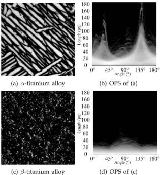
(a) α-titanium alloy 0 60 20 40 0° 45° 90° 135° 180° 80 100 120 140 160 Length (px) Angle (°) (b) OPS of (a) (c) β-titanium alloy 0 60 180 20 40 0° 45° 90° 135° 180° 80 100 120 140 160 Length (px) Angle (°) (d) OPS of (c)

Fig. 4. Oriented pattern spectrum for α- and β- titanium alloys. See the text for explanation.

structure of an ordered group.

The complexity is studied in section 5 and this algo-rithm is applied to 2-D images in the next section.

4

A

2-D

It will be explained in this section how to apply the pre-vious algorithm to 2-D images, by means of partitioning the image support into thin straight lines, at arbitrary orientations. This strategy is applied to the computation of Oriented Pattern Spectrum (OPS) [7]. Finally, some hints to compute the 2-D component tree are given.

In this section, g : E → V is a 2-D image, where E is rectangular domain of Z2 _{of the sort [1, N}

1] × [1, N2],

and V , as previously, is equal to Z or R.

4.1 2-D image scanning strategy

Alg. 2 takes one pixel as input, and is clearly indepen-dent of the orientation of the line. Hence, we can apply it to 2-D images, provided we have an appropriate image-scanning strategy. Soille et al. [25] described a way to go through all pixels of an image at a given orientation, by using Bresenham lines [26]. Moreover, they addressed the padding problems by adding constraints to avoid any overlaps between two translated lines. Hence, the logic behind the construction of these lines ensures that each pixel will be processed only once. This allows the algorithm to run in place. For openings in arbitrary orientation, we add a line buffer to store the index position of all the previous pixels of the line. Hence, we could easily write the result of the filter in the output image with no other extra computation.

Hereafter, image g is decomposed into a set of 1-D signals {gα,k}k∈K, following direction α.

4.2 Oriented Pattern Spectrum

We have seen that the local orientation on a given pixel of a 2-D image can be measured by the supremum of lin-ear openings. We may wish to additionally measure the pattern spectrum for each orientation, which leads to the Oriented Pattern Spectrum (OPS), initially introduced by Maragos [7]:

OPS(g)(λ, α) = X

k∈K

(PS(gα,k))(λ). (13)

Computing the OPS can be very time consuming. Using the presented algorithm reduces its computation time. Fig. 4 illustrates the results of this operator. Ori-ented pattern spectra are represOri-ented as 2-D images, one column for each orientation. Fig. 4 (b) and (d) show the OPS of the (a) α- and (c) β- titanium alloys, respectively. We can see in (b) two peaks, giving evidence of an alignment in the image. The majority of the structures are oriented around 140◦ _{(measured anticlockwise from}

the horizontal line), with a second peak around 40◦_.

The majority of the structures are up to 80 pixels long, with several individuals from 120 to 160 pixels long. The β-titanium alloy is rather isotropic, with only a slight alignment around 90◦_.

4.3 Border effects

Consider a stationary, random process ξ of arbitrarily placed, L-pixel long, non intersecting and non over-lapping, straight lines, oriented in a constant direction ϑ. The P S(ξ) in the direction of ϑ is δ(L), the Dirac function at L. Now, consider a bounded, discrete support [1, N ]2_⊂Z2_{, and the realisation of ξ on D, see Fig. 5. The}

intersection with a finite support introduces in the P S a bias (a.k.a. border effects) due to the truncation of the structures in ξ (see the red curve in Fig. 5).

0 100 000 200 000 300 000 400 000 0 50 100 P a tt e rn s p e ct ru m ( v o lu m e ) 0 50 100 Length (px)

Fig. 5. Randomnly placed, 100-pixel long, straight lines and the pattern spectrum: blue - expected pattern spec-trum, red - effect of truncation on a bounded support.

The border effect is an ubiquitous problem, differently handled in various applications. Van Droogenbroeck [19] proposes an interesting discussion. He recommends to add the maximal value of V (let us call it ∞) outside the image support. On the other hand, in the domain of connected filters, one often completes by adding the minimal value of V .

In granulometries one often uses padding by ∞. In-deed, ∞ is a recessive value that allows considering in Eq. 7 the truncated structures (of unknown length) as infinitely long, and makes them unaffected by γν, for

any ν < ∞.

The proposed algorithm can easily handle both border management strategies. Considering the infinite exten-sion, every cord touching the border is ignored. For openings, the flag Passed of the first cord pushed into the stack and the cords remaining in the stack at the end of the line, must be set to true. The timings stay unchanged with this strategy.

4.4 2-D component tree

If we compute a tree for each 1-D image gα,k obtained

from the 2-D image g, we get a set of trees called a forest. On its own, such a forest is not interesting, since it does not describe the 2 dimensional patterns of the images. However, Wilkinson et al. [27], and later Matas et al. [28], [29] have described a method to merge all these trees to get the 2-D component tree of the image. Hence, the proposed algorithm can be seen as a part of a new process to get the 2-D component tree in an efficient way.

5

C

The computational complexity of this algorithm is evalu-ated focusing first on the 1-D algorithm. Then, we study the 2-D part.

5.1 1-D scan strategy

Consider a 1-D signal f : [1 . . . N ] → V , with V = Z or R. The input signal is read sequentially from left to right (Alg. 1, lines 4 to 6) and it calls Alg. 2 once per every sample.

By analysing Alg. 2, we notice that every cord, where it starts, is pushed once and only once into the LIFO stack (line 2), and eventually retrieved (line 5), when it ends. The retrieval is done in a cycle while (line 4) since several cords may end simultaneously at one downfalling edge (as e.g. the cords c2 and c5 in Fig. 3). The cycle while,

executes once per every cord. All remaining operators in the Alg 2 are O(1) operations, like tests or operations on the stack.

Hence, we may conclude, that Alg. 2 executes with the average complexity of O(1) per pixel. However, because of the conditions the execution time differs according to the content of the image. The time will decrease for smooth signals. The theoretical lower bound is reached with constant signals, containing only one cord.

Regarding memory consumption, the maximum number of cords pushed into the stack is bounded by the mini-mum between the number of grey levels and the number of pixels of the signal.

In the following paragraph, we will analyse the com-plexity for 2-D supports.

5.2 2-D scan strategy

We perform a complete scan of a 2-D rectangular image with a set of parallel, α-oriented Bresenham lines. With the Soille algorithm, this is done in O(1) per pixel. Furthermore, this set of lines can be computed in parallel since each line is independent from the others.

Therefore, the complexity does not increase with the size of the openings λ and every pixel is computed in a constant time. Next section is devoted to a comparison of the timings with the state of the art.

6

T

Beside its adaptability, this algorithm is designed for speed. Thus, this section is devoted to compare this algorithm with the state of the art for openings, gran-ulometries and oriented size distributions. All these ex-periments have been made on a laptop computer using only one thread (Intel Core 2 Duo T7700 CPU @2.4GHz).

6.1 Timings for openings

Four benchmarks on openings have been computed to test the speed of the proposed algorithm. First, we see the correlation between the computation time and the image content. Then, we compare openings in arbitrary orientations for different algorithms. Finally, we make a benchmark with reference to the orientation and with reference to different input data types.

6.1.1 Benchmark with the image content

By analysing Alg. 2, we note that the number of op-erations changes with the image content. Hence, we measure the average time for 1000 horizontal openings for different images of size 512×512 pixels: Goldhill, two other versions of Goldhill (where the number of grey levels has been set to 2 and 9, with no dithering), an uniformly distributed random noise image and, finally, a constant signal.

Fig. 7 collects the results. As expected, the constant image gives the smallest computation time. We also note that an image with uniform noise is computed faster than Goldhill image. A general rule for this algorithm is that timings are correlated to the mean number of pixels into the stack. A random signal will have, in average, fewer pixels in the stack than a natural image. Furthermore, the fewer cords there are, the closer you get to the theoretical lower bound.

6.1.2 Benchmark with other algorithms

For a comparison with the state of the art, we use five other algorithms. The first one is an algorithm by Van Herk, Gil and Werman [16], [17] (referred to as HGW algorithm hereafter). Then, we use Clienti et al.’s algorithm [18] (Clienti), Van Droogenbroeck et

(a) (b) (c) (d) (e)

Fig. 6. Image of size 512 × 512 used for Fig. 7. (a) goldhill, (b) goldhill with 9 grey levels, (c) goldhill with 2 grey levels, (d) random noise and (e) a constant image

0 1 2 3 4 5 6 0 50 100 150 T im e (m s) Goldhill Random Noise Goldhill 9 grey levels Goldhill 2 grey levels Constant image

0 50 100 150

Size of the opening : λ (pixels)

Fig. 7. Timings for horizontal openings of size λ for different images, using the proposed algorithm (512 × 512 pixels)

al.’s algorithm [16], [30] (Van Droogenbroeck), Bartovsk ´y et al.’s algorithm [20] (Bartovsky) and finally a naive implementation that follows the classical definition of an opening (Naive). All these algorithms have a O(1) complexity per pixel, excepted the naive algorithm O(λ). They have been integrated to the same platform, in C++, with exactly the same interface. Then, we average the computation time of 1000 realisations of openings with arbitrary orientations. The timings have been computed on Goldhill image (Fig. 8) but we note that the results are approximately the same with other images.

The difference between the naive implementation and others methods is huge. The naive implementation’s complexity is independent on the image content but it does depend on the length of the openings. Our algorithm is very fast. However, Van Droogenbroeck’s method outperforms our algorithm, especially for large values of λ. One reason can be pointed out to explain this difference; for our algorithm, every pixel of the output image is written exactly once. This can slow down our algorithm compared to an algorithm that only writes the modified pixels. We note, however, that Van Droogenbroeck’s algorithm is not able to handle efficiently 16 bits or floating-point data images.

6.1.3 Benchmark with orientation

Openings in arbitrary orientation require an extraction of the lines. We use the same method for all the algorithms

0 5 10 15 20 25 30 0 50 100 150 T im e ( m s) Naive HGW Clienti Bartovsky This paper Van Droogenbroeck 0 50 100 150

Size of the α-oriented openings: λ (pixels)

Fig. 8. Timings for openings in arbitrary orientation with regard to λ for different algorithms (Goldhill image)

0 5 10 15 0 10 20 30 40 50 60 70 80 90 T im e (m s) HGW Bartovsky Clienti This paper Van Droogenbroeck 0 10 20 30 40 50 60 70 80 90

Orientation of the opening (degrees)

Fig. 9. Timings for openings with regard to the orientation for different algorithms (Goldhill image 512 × 512 pixels)

[25] excepted for the Bartovsk ´y algorithm, which uses its own line extraction. We average the computation time of 1000 openings, for every orientation with λ = 41 pixels. Fig. 9 collects the results and we note that the compu-tation times are almost independent of the oriencompu-tation. The angle α = 0◦ and α = 90◦ are different since the extraction of the lines is straightforward. We note that the best situation for all the algorithms is α = 0◦ _as

expected. This is due to the row major organisation of our data, which minimises cache misses.

6.1.4 Benchmark with input data types

All the previous experiments have been computed with 8-bit images. This benchmark allows visualising the overhead introduced by using other input data type: 8-, 16-, 32-bit, floating point (single and double precision) for the computation of a horizontal opening. To avoid any bias introduced by the image content, we use a random uniform noise image of size 512 × 512 for our experiments. We compute the average time of 1000 open-ings for each input data type.

Note that the algorithm proposed by Van Droogen-broeck – the fastest for 8-bit images – does not support

0 2 4 6 8 10 12 14

UINT8 UINT16 UINT32 float double

T im e ( m s) HGW Clienti Bartovsky This paper Van Droogenbroeck

UINT8 UINT16 UINT32 float double

Fig. 10. Timings for openings with regard to the input data type (Uniform noise image 512 × 512 pixels)

2048 x2048 4096 x 4096 8192 x 8192 0 200 400 600 800 1000 1200 0 20 40 60 80 T im e (m s) Vincent This paper 0 20 40 60 80

Number of pixels (MPixel)

Fig. 11. Timings for horizontal granulometries with refer-ence to the image size. The proposed algorithm outper-forms the algorithm by Vincent (Uniform noise images).

any other data type, hence, we have not included it into this benchmark. The results are depicted in Fig. 10. We note that our algorithm is the fastest.

6.2 Timings for granulometries

Compared to a naive implementation, the algorithm by Vincent for granulometries is highly efficient [21]. Even many years after its publication, it used to be the fastest algorithm for 1-D granulometries. We have compared these two algorithms and the timings are collected in Fig. 11, where we plot the average time needed to build a horizontal pattern spectrum with reference to the number of pixels of the signal. Our method is 21% faster than Vincent’s one, which becomes useful when we compute the oriented size distribution. The OPS requires many linear granulometries in all orientations: we may need to compute 180n−1 _{granulometry for n-D}

images. The computation times for the OPS of images 4(a) (322x322) and 4(c) (625x625) are respectively equal to 0.37s and to 1.06s for 180 orientations.

7

C

This paper introduces a new, flexible and efficient algo-rithm for computing 1-D openings and granulometries. Its theoretical complexity is linear with respect to the number of image pixels, and constant with respect to the opening size. Moreover, it can be applied to a large set of image types; in fact, the image values only need to have the structure of an ordered group. Extensive benchmarks show that it is the fastest algorithm for com-puting 1-D openings on images whose data precision is higher than 8 bits (for 8-bit images, the algorithm by Van Droogenbroeck remains unvanquished). It can also be used to compute 1-D granulometries, running faster than the algorithm proposed by Vincent, which has led this category for many years. Moreover, 1-D component trees can also be efficiently computed with the same algorithm. From a software engineering point of view, it should be noted that having the same algorithm for computing different operators, with different data pre-cisions, is very interesting. Futhermore, one can choose between two border extensions to adapt these operators to applications.

The proposed algorithm is applied to 2-D images in several ways: i) the classical linear openings for oriented filtering and/or enhancing of linear structures; ii) the collection of size distributions for all orientations gives the oriented pattern spectrum.

In the future, we shall focus on the computation of lo-cal granulometries for analysing non-stationary signals, or to segment textured images. A second extension is to introduce new scan strategies, beyond straight direc-tions, and use this algorithm to efficiently compute path openings. Finally, small modifications of this algorithm are required to compute openings by reconstruction for 1-D signals.

R

[1] J. Serra, Image analysis and mathematical morphology. Academic Press, 1982, vol. 1.

[2] ——, Image analysis and mathematical morphology. Academic Press, 1988, vol. 2 Theoretical Advances.

[3] C. Heneghan, J. Flynn, M. O’Keefe, and M. Cahill, “Charac-terization of changes in blood vessel width and tortuosity in retinopathy of prematurity using image analysis,” Medical image analysis, vol. 6, no. 4, pp. 407–429, 2002.

[4] B. Obara, “Identification of transcrystalline microcracks observed in microscope images of a dolomite structure using image analysis methods based on linear structuring element processing,” Com-puters & geosciences, vol. 33, no. 2, pp. 151–158, 2007.

[5] G. Matheron, Random sets and integral geometry. Wiley New York, 1975, vol. 1.

[6] S. Batman, E. R. Dougherty, and F. Sand, “Heterogeneous mor-phological granulometries,” Pattern Recognition, vol. 33, no. 6, pp. 1047–1057, 2000.

[7] P. Maragos, “Pattern spectrum and multiscale shape representa-tion,” Pattern Analysis and Machine Intelligence, IEEE Transactions on, vol. 11, no. 7, pp. 701–716, 1989.

[8] N. Theera-Umpon and P. D. Gader, “Counting white blood cells using morphological granulometries,” Journal of Electronic Imag-ing, vol. 9, pp. 170–177, 2000.

[9] S. Outal, D. Jeulin, and J. Schleifer, “A new method for estimating the 3d size-distribution-curve of fragmented rocks out of 2d images,” Image Analysis and Stereology, vol. 27, pp. 97–105, 2008.

[10] P. Salembier, A. Oliveras, and L. Garrido, “Antiextensive con-nected operators for image and sequence processing,” Image Processing, IEEE Transactions on, vol. 7, no. 4, pp. 555–570, 1998. [11] P. Salembier and J. Serra, “Flat zones filtering, connected

op-erators, and filters by reconstruction,” Image Processing, IEEE Transactions on, vol. 4, no. 8, pp. 1153–1160, 1995.

[12] R. Jones, “Connected filtering and segmentation using component trees,” Computer Vision and Image Understanding, vol. 75, no. 3, pp. 215–228, 1999.

[13] B. Naegel and L. Wendling, “A document binarization method based on connected operators,” Pattern Recognition Letters, vol. 31, no. 11, pp. 1251–1259, 2010.

[14] M. Couprie, L. Najman, and G. Bertrand, “Quasi-linear algorithms for the topological watershed,” Journal of Mathematical Imaging and Vision, vol. 22, no. 2, pp. 231–249, 2005.

[15] J. Pecht, “Speeding-up successive minkowski operations with bit-plane computers,” Pattern Recognition Letters, vol. 3, no. 2, pp. 113–117, 1985.

[16] M. Van Herk, “A fast algorithm for local minimum and maximum filters on rectangular and octagonal kernels,” Pattern Recognition Letters, vol. 13, no. 7, pp. 517–521, 1992.

[17] J. Gil and M. Werman, “Computing 2-d min, median, and max filters,” Pattern Analysis and Machine Intelligence, IEEE Transactions on, vol. 15, no. 5, pp. 504–507, 1993.

[18] C. Clienti, M. Bilodeau, and S. Beucher, “An efficient hardware architecture without line memories for morphological image processing,” in Advanced Concepts for Intelligent Vision Systems. Springer, 2008, pp. 147–156.

[19] M. Van Droogenbroeck and M. Buckley, “Morphological erosions and openings: fast algorithms based on anchors,” Journal of Math-ematical Imaging and Vision, vol. 22, no. 2, pp. 121–142, 2005. [20] J. Bartovsk ´y, P. Dokl´adal, E. Dokl´adalov´a, and M. Bilodeau, “Fast

streaming algorithm for 1-D morphological opening and closing on 2-D support,” in Mathematical Morphology and Its Applications to Image and Signal Processing, ser. LNCS, vol. 6671. Springer, 2011, pp. 296–305.

[21] L. Vincent, “Granulometries and opening trees,” Fundamenta In-formaticae, vol. 41, no. 1-2, pp. 57–90, 2000.

[22] L. Najman and M. Couprie, “Building the component tree in Quasi-Linear time,” Image Processing, IEEE Transactions on, vol. 15, no. 11, pp. 3531–3539, 2006.

[23] D. Menotti, L. Najman, and A. de Albuquerque Ara ´ujo, “1d component tree in linear time and space and its application to gray-level image multithresholding,” in Proceedings of the 8th International Symposium on Mathematical Morphology, 2007, pp. 437– 448.

[24] V. Morard, P. Dokl´adal, and E. Decenci`ere, “Linear openings in arbitrary orientation in o(1) per pixel,” in Acoustics, Speech and Signal Processing (ICASSP), IEEE International Conference on. IEEE, 2011, pp. 1457–1460.

[25] P. Soille, E. J. Breen, and R. Jones, “Recursive implementation of erosions and dilations along discrete lines at arbitrary angles,” Pattern Analysis and Machine Intelligence, IEEE Transactions on, vol. 18, no. 5, pp. 562–567, 1996.

[26] J. Bresenham, “Algorithm for computer control of a digital plot-ter,” IBM Systems journal, vol. 4, no. 1, pp. 25–30, 1965.

[27] M. H. F. Wilkinson, H. Gao, W. H. Hesselink, J. E. Jonker, and A. Meijster, “Concurrent computation of attribute filters on shared memory parallel machines,” Pattern Analysis and Machine Intelligence, IEEE Transactions on, vol. 30, no. 10, pp. 1800–1813, 2008.

[28] P. Matas, E. Dokl´adalov´a, M. Akil, T. Grandpierre, L. Najman, M. Poupa, and V. Georgiev, “Parallel algorithm for concurrent computation of connected component tree,” in Advanced Concepts for Intelligent Vision Systems, ser. LNCS. Springer, 2008, vol. 5259, pp. 230–241.

[29] P. Matas, E. Dokl´adalov´a, M. Akil, V. Georgiev, and M. Poupa, “Parallel hardware implementation of connected component tree computation,” in Field Programmable Logic and Applications (FPL), 2010 International Conference on, 31 2010-sept. 2 2010, pp. 64 –69. [30] R. Dardenne and M. Van Droogenbroeck, “libmorpho,

http://www.ulg.ac.be/telecom/research.html.” [Online]. Avail-able: http://www2.ulg.ac.be/telecom/research/libmorpho.html

Vincent Morard is a PhD candi-date at the Centre of Mathematical Morphology, the School of Mines in Paris, France. He is graduated from the engineering school CPE in Lyon, France, in 2009, as an engineer spe-cialised in computed science and im-age processing. His research inter-ests include mathematical morphol-ogy, noise reduction, pattern recogni-tion and statistical learning.

Petr Dokladal is a research engineer at the Centre of Mathematical Mor-phology, the School of Mines in Paris, France. He graduated from the Tech-nical University in Brno, Czech Re-public, in 1994, as a telecommunica-tion engineer and received his Ph.D. degree in 2000 from the University of Marne la Vall´ee, France, in general computer sciences, specialized in im-age processing.

His research interests include medical imaging, image segmentation, mate-rial control and pattern recognition.

Etienne Decenci`ere received the en-gineering degree in 1994, the Ph.D. degree in mathematical morphology in 1997, both from MINES ParisTech, and the Habilitation in 2008 from the Jean Monnet University. He holds a research fellow position at the Cen-tre for Mathematical Morphology of MINES ParisTech.

His main research interests are in mathematical morphology, image segmentation, non-destructive testing, and biomedical applications.