An approximate folk theorem with imperfect private information

Digitized

by

the

Internet

Archive

in

2011

with

funding

from

Boston

Library

Consortium

IVIember

Libraries

working paper

department

of

economics

AN APPROXIMATE FOLK THEOREM WITH IMPERFECT PRIVATE INFORMATION

Drew Fudenberg and David K. Levine No. 525 March 1989

massachusetts

institute

of

technology

50 memorial

drive

Cambridge,

mass.

02139

AN APPROXIMATE FOLK THEOREM WITH IMPERFECT PRIVATE INFORMATION

Drew Fudenberg and

David K. Levine

AN APPROXIMATE FOLK THEOREK WITH

IMPERFECT PRIVATE INFORMATION by Drew Fudenberg and *** David K. Levine March 1989 *

We are grateful to Andreu Mas-Colell. NSF Grants 87-08616 and

86-09697 and a grant from the UCLA Academic Senate provided financial

support. **

Department of Economics, Massachusetts Institute of Technology

***

Department of Economics, University of California, Los Angeles; part

Abstract

We give a partial folk theorem for approximate equilibria of a class

of discounted repeated games where each player receives a private signal of

the play of his opponents . Our condition is that the game be

"informationally connected," meaning that each player i has a deviation

that can be statistically detected by player j regardless of the action of

any third player k. Under the same condition, we obtain a partial folk

theorem for the exact equilibria of the game with time-average payoffs,

JEL Classification numbers = 022, 026

Keywords: Repeated games, folk theorem, private information,

1. Introduction

We give a partial folk theorem for the approximate equilibria of a

class of repeated games with imperfect information satisfying an

informa-tional linkage condition. Every payoff vector which exceeds a mutual threat

point and is generated by one-shot mixed strategies from which no player can

profitably deviate without having some effect on other players, is

approxi-mately an approximate sequential equilibrium payoff if the discount factor

is close enough to one.

The class of repeated games we consider has complete but imperfect

information. Each period, player i chooses an action a , then observes

his own payoff and also a signal z of the play of his opponents. This

model includes as a special case games of imperfect public information as

defined by Fudenberg-Levine-Maskin [1989]. In these games, there is a

publicly observed variable y, and each player i observes z. - (y,a.).

The public information case includes the literature on repeated oligopoly

(Green-Porter [1983], Abreu-Pearce Stacchetti [1986]), repeated

principal-agent games (Radner [1981, 1985], Rubinstein-Yaari [1983]), repeated

partnerships (Radner [1986], Radner-Myerson-Maskin [1986]), as well as the

classic case of observable actions (Auman-Shapley, Friedman [1971],

Rubinstein [1981], Fudenberg-Maskin [1986]). It also includes the examples

studied in the literature of repeated games with "semi-standard

information", as discussed in Sorin [1988].

While examples of repeated games that have been formally studied have

public information, players have private information in some situations of

economic interest. Indeed, the central feature in Stigler's [1961] model of

secret price-cutting is that each firm's sales depend on the prices of its

to show that a partial folk theorem extends to these cases, provided we

relax the notion of equilibrium slightly.

The key element in any folk theorem is that deviators must be punished.

This requires, with three or more players, that non-deviators coordinate

their punishments, and may even require a player to cooperate in his own

punishment. With public information, the necessary coordination can be

accomplished by conditioning play on the commonly observed outcome. When

players receive different private signals they may disagree on the need for

punishment. This raises the possibility that some players may believe that

punishment is required while others do not realize this. The most

straight-forward way to prevent such confusion from dominating play is to

periodically "restart" the strategies at commonly known times, ending

confusion, and permitting players to recoordinate their play. This,

however, makes it difficult to punish deviators near the point at which play

restarts and forces us toward approximate equilibrium.

The use of approximate equilibrium leads to an important

simplification, because it allows the use of review strategies of the type

introduced by Radner [1981]. Under these strategies, each player calculates

a statistic indicating whether a deviation has occurred. If the player's

statistic crosses a threshold level at a commonly known time, he

communica-tes this fact during a communication stage of the type introduced by Lehrer

[1986]. Our informational linkage condition ensures that all players

cor-rectly interpret this communication, so that the communications stage allows

coordination of punishments. The importance of approximate equilibrium is

that Radner-type review strategies do not punish small deviations, i.e.,

those that do not cause players statistics to cross the threshold level.

consequence of approximate equilibrium is that sequentiality loses its

force, and the review strategies are perfect whenever they are Nash. This

is because punishments end when the strategies are restarted so the cost to

punishers is small. Thus the punishment are "credible" in the sense that

carrying them out is an approximate equilibrium.

Our results are closely connected to those of Lehrer [1986, 1988a,b,c,d,

1989] who considers time-average Nash equilibrium of various classes of games

with private information and imperfect monitoring but with non-stochastic

out-comes. In addition to the deterministic nature of outcomes, Lehrer's work has

a different emphasis than ours, focusing on completely characterizing

equilibrium payoffs under alternative specifications of what happens when a

time average fails to exist. Our work provides a partial characterization of

payoffs for a special but important class of games.

A secondary goal of our paper is to clarify the correction between

Lehrer's work and other work on repeated time-average games, and work on

discounted games such as ours. In particular we exposit. the connection

between approximate discounted equilibrium and exact time-average

equilib-rium, which is to some extent already known to those who have studied

repeated games. We emphasize the fact that the time-average equilibrium

payoff set includes limits of approximate as well as exact discounted

equilibria. Although we show that the converse is false in general, the

type of construction used by Lehrer (and us) yields both an approximate

discounted and a time-average theorem. For economists, who are typically

hostile to the notion of time-average equilibrium, we hope to make clear

that results on repeated games with time-average payoffs are relevant,

If we consider the set of equilibrium payoffs as potential contracts in

a mechanism design problem, there is an interpretation of approximate

equi-librium that deserves emphasis. The set of equilibrium payoffs in our

theorem in some cases strictly exceeds that for exact equilibria. This

means that exact equilibrium may be substantially too pessimistic. The

efficiency frontier for contracts may be substantially improved if people

can be persuaded to forego the pursuit of very small private benefits. For

example, even if ethical standards have only a small impact on behavior,

they may significantly improve contracting possibilities.

Section 2 of the paper lays out the repeated games model. Section 3

establishes a connection between approximate sequential discounted

equilibria with discount factor near one, and time-average equilibrium. In

particular, both types of equilibria can be constructed from finite-horizon

approximate Nash equilibria. Section 4 describes our informational linkage

condition, and proves a partial folk theorem,

2. The Model

In the stage game, each player i, i - 1 to N, simultaneously

chooses an action a. from a finite set A. with m. elements. Each

player observes an outcome_' z.

11

1

let z - (z, z ) and Z - x. ,Z.. Each action profile a e A X. ,A,

1 n 1-1 i 1-1 1

induces a probability distribution tt (a) over outcomes z. Each player

i's realized payoff r (z.) depends on his own observed outcome only; the

opponents' actions matter only in their influence on the distribution over

outcomes.

Player i's expected payoff to an action profile a is

g. (a) - S TT (a)r. (z.) .

"i _ z 1 1

We also define d - max g.(a.,a .) - _{g.(a', ,a .) to} be the maximum

i,a. ,a: ,a .

1 1 -1

one-period gain any player could obtain by playing one of his actions a

instead of another al .

We will also wish to consider various types of correlated strategy

profiles. A correlated action profile a is simply a probability

distribu-tion over A. We write a for the induced probability distribution over

A , H X. . A . A belief by player i is such a probability distribution,

and the vector (a. ,a ) represents the correlated action in which player

i plays a and the other players correlate according to a . . We also

write a for the marginal induced over A by a. If the play of players

is independent, we refer to a as a mixed action profile, in which case a

is characterized by and may be identified with (a. a ), the vector of

marginals

.

For any correlated action profile a, we can calculate the induced

distribution over outcomes

TT (a) - 2 TT (a)a(a).

aGA

We can also calculate the marginal distribution over player i's outcomes

TT (z ,q:) - S T (q).

Finally, we may calculate the expected payoff to player i

g (a) - E TT (z ,Q)r (z ) - Z TT (a)r.(z ).

z.eZ, . ^ ^ ^ ZGZ ^ ^

1 i

In the repeated game, in each period t - 1,2 the stage game is

played, and the corresponding outcome is then revealed. The history for

let h.(0) denote the null history existing before play begins. A strategy

for player i is a sequence of maps a.(t) mapping his private history

h.(t-l) to probability distributions over A .

A system of beliefs b, for player i specifies for each time t and

private history h.(t), a probability distribution b.(h.(t)) over private

histories of other players of length t. A profile of beliefs b for all

payers is consistent with the strategy profile a, if for every finite time

horizon the truncation of b is consistent with the truncation of a in

the sense of Kreps-Wilson [1982]. This requires that there exists for each

T T

truncation T a sequence of truncated strategy profiles a -* a , putting

strictly positive probability on every action, such that the unique sequence

T T

of truncated belief profiles derived from Bayes law, b - b .

Given a system of beliefs b and a history h (t) a distribution is

induced over the history of all players play. Given this distribution and

the strategy profile a, a corresponding distribution is induced over play

at all times r. In turn this gives an expected payoff in period r to

player i, which we denote by G. (r ,h. (t) ,b. ,a) . The corresponding

normalized present value to player i at discount factor < 5 < 1 is

Wj^(h^(t).b^,a.5) - (1-5) 2"_^ 5^'^ G(r ,h^(t) ,b^,a).

^

While if

5-1

wj(hj^(t).b.,a) - (1/T) Sy_^ G^(r,h^(t),b^,a)

and

W (h (t),b ,cr,l) - lira sup W^Ch (t) ,b ,a) .

^ _^

T-*«

value of time average expected payoff is the same for all beliefs consistent

T

with a. The emphasize this, we write W (cr,5) and W. (a) in place of

W^(h^(0),b^,a,6) and W^(h^(0) ,b^.a)

.

For 5 < 1, a strategy profile a is an e-Nash equilibrium if for

each player i and strategy a'

(2.1) W^((aj^.a_^),fi) ^ W^(£7,5) + £

There is also a corresponding notion of a truncated e-Nash equilibrium,

where we require

W^(aj^,a_^) < W^(a) + e.

An £-sequential equilibrium is defined in a similar way, except that we

require there exist beliefs b consistent with a such that

(2.2) W^(h^(t),b^,(a^,a_^),5) < W^(h^(t) .b^^.a, 5) + 8^''^e

for all players i, and all histories h. (t) (not merely the null initial

history). Notice that W, is measured as a present value at time 1,

rather than time t. Consequently, an €-sequential equilibrium is defined

so that the gain to deviating at time t is of order e, in time-t units.

Notice that this definition is stronger than the usual version, found in

Fudenberg and Levine [1983] , for example: ordinarily the gain to deviating

at time t is measured in time-0 units, not time-t units.

For

5-1,

A uniform Nash equilibrium is a profile a such that

T

(2.3) W.(cr) converges, and

(2.4) for all p > 0, 3r, such that T > r implies

wT(cr: ,a .) < wT(cr) + p.

A uniform sequential equilibrium is a profile a such that

T

(2.5) W. (h. (t) ,b ,a) converges for all histories h.(t) and

consistent beliefs b, and

(2.6) there exist consistent beliefs b such that for all p > 0,

3r such that T > r implies for all histories h.(t) and

strategies a.

,

W^(h.(t),b.,(al^,a_.) < wj(h^(t),b.,a) + p.

When a satisfies condition (2.3) we call it repular: if it satisfies (2.5)

we say it is sequentially regular.

Our definitions of time average equilibrium require that the

appropriate regularity condition be satisfied. In other words, we have

required that the time-average payoff exist if no player deviates, and that

there be a uniform bound on the gain to deviating in any sufficiently long

subgame. Both conditions are responses to our unease in comparing lim infs

or lim sups of payoffs when the limit does not exist. We impose the

condi-tions because we interpret time averaging as the idealized version of a game

with long finite horizon or very little discounting. Below we show that

non-uniform equilibria cannot always be interpreted in this way.

3. Discounting and Time Averaging

Out goal is to characterize the set of equilibrium payoffs when players

are very patient. In the next section we characterize truncated €-Nash

equilibrium payoffs with small £ as containing a certain set V*. Since

this notion of equilibrium is not the most economically meaningful, we first

show that this is in fact a strong characterization of payoffs.

Theorem 3.1: Suppose there exists a sequence of times T , non-negative

numbers e -^ _{and strategy profiles} a such that a is a T -truncated

T

time-average e -Nash equilibrium and W (a ) - v. . Then

(A) There exists a sequence of discount factors 5

-I,

n_,

,,

n.

numbers t - and strategy profiles a such that a is an £

-sequential equilibrium for 6 and W. (a ,5 ) -* v. .

(B) There exists a uniform sequential equilibrium strategy profile a such

that W (cr.l) - V

Remark 1: It is well known that the hypotheses of the theorem imply that s

is a time-average Nash equilibrium (see for example, Sorin [1988]).

Remark 2: The hypothesis is weak in the sense that only approximate Nash

equilibria are required. However, as long as we consider approximate

equi-librium, or infinite time-average equilibrium, (A) and (B) show that

sequentlality has little force. Roughly, the reason is that after a

deviation, no further deviations are anticipated, so the cost of punishment

must be only paid once. This has negligible cost if players are very

patient. It is easily seen in the following example, which is a special

case of the main theorem in the next section. Consider a game in which

players perfectly observe each others past play, and suppose there is a pure

action profile a for which g(a) strictly exceeds the minmax for all

players. Clearly there is a discount factor 1 > 5, > and number of

periods K, such that if 5 > £ the loss to each player of being minraaxed

by his opponents for K periods exceeds any possible one-shot gain of

deviating from a. Consider then a strategy profile consisting of a review

phase in which all players play a, and n different punishment phases in

10

game is in the review phase, and the review phase continues as long as no

player deviates, or more than one player deviates simultaneously. Whenever

a single player deviates, a punishment phase against that player immediately

begins. The punishment phase continues K periods, regardless of whether

any further deviation occurs, then the game restarts with a new review

phase. Since no player can profitably deviate during a review phase for

6 > £, these strategies form a Nash equilibrium with payoffs g(a) . It is

equally clear that they are not generally sequential (subgame perfect)

,

because players may profitably deviate during punishment phases.

In proving the folk theorem, Fudenberg-Maskin (1986a) construct

strategies that induce the players to carry out punishments by providing

"rewards" for doing so. But such rewards are not provided by our review

strategies. Indeed, the Fudenberg-Maskin construction is only possible if the

game satisfies a "full-dimensionality" condition that we have not imposed.

Thus the conclusion of (A) cannot in general be strengthened to £ - 0.

The review strategies do, however, form an €(5)-sequential equilibrium

with £(5) -+ _as 5 -* _{1. (Note that with observable actions, sequential}

equilibrium and subgame -perfect equilibrium are equivalent.) To show this, we

need only calculate the greatest gain to deviating during a punishment phase.

Recall that d is the greatest one-shot gain to any player of deviating from

any profile. Consequently, the gain is at most (l-5)Kd, which.clearly goes

to zero as 6 -> _{1. The point is that the punishment lasts only K periods, and}

players never expect to engage in punishment again. Consequently, with

extreme patience, the cost of the punishment is negligible. In particular,

with time-averaging this is an exact equilibrium.

Proof of (A) : Consider the strategy a of playing a from 1 to T

,

11

We call period 1 to t" "round 1", t" + 1 to 2t" "round 2" and so on.

Fix 5 < 1 and any beliefs consistent with a . Let a history

(h^ (t) h (t)) be given. Let us calculate an upper bound on any

player's gain to deviating in time-t normalized present value. Fix a time

t and a history (h^ (t) , . . . ,h (t)), and choose k so that

kT < t < (k+l)T , so that t is in round k. Since the maximum of

per-period gain to deviating is d, we know that regardless of the history, no

player by deviating in round k, can gain more than (1-5)T d. Further,

play from time (k+l)T

+1

previous rounds. Since round k+1 is a truncated time-average e -Nash

equilibrium, at most (1-6)T e can be gained by deviating in this round.

During round k+2 at most 5(1-5)T e can be gained, and so forth.

Conse-T

quently, no player can gain more than (1-5)T (d+e /(1-fi )). As

5-+1,

this quantity approaches e by I'Hopital's rule. Clearly, then, we may

choose S close enough to 1 that a is a 2e -sequential equilibrium.

In addition, because of the repeated structure of a , it is clear that

T

W.(a",5")

11

1 i

Proof of (B) : Consider the strategy a of playing a from 1 to T ,

2 1

12

a from T -t- 1 to T + T , and so forth. Fix any beliefs consistent

with a. Let a history (h.. (t) , . . . ,h (t)) be given and let t be in round

k. By deviating in the current round, player i can gain at most d per

period as play in the future is independent of play in this round. The

per-k+1 k+2

period gain at k+1 is at most e ,' in round k+2, e . Since

k

€ -* , this implies that the time average gain is zero. Since

T

k k

W. (a ) -> V. , s is a uniform sequential equilibrium, and this yields the

12

Each of the two conclusions of Theorem 3.1 has strengths and weaknesses.

The limit of discounting is more appealing than time-averaging, which suggests

the interpretation (A) , but exact equilibrium is more appealing than

approximate equilibrium, which suggests the interpretation (B) . In this

context, it is worth emphasizing reiterating that the conclusion of (A) cannot

be strengthened to e

=0.

of time-average equilibria includes not only the limits of exact discounted

equilibria, but the limits of approximate discounted equilibria as well.

If we weaken definition (2.6) to allow the gain to deviating, p, to

depend on T and t, we have a time-averape sequential equilibrium, rather

than a uniform one. That these equilibria include all limits of discounted

sequential equilibria as shown by

Proposition 3.2: If a is sequentially regular, and is an e(5)-sequential

equilibrium for discount factor 5 with e(5) -+ _0, then _{a is a}

time-average sequential equilibrium.

Proof: This effectively follows from the fact that the limit points, as

5 - 1 , of the normalized present value of a sequence of payoffs are

contained in the set of limit points of the finite time averages. This

implies that if a is sequentially regular, then the discounted value of

payoffs along the continuation equilibrium approaches the value with time

averaging. Deviations from the continuation payoff when evaluated with the

discounting criterion yield values whose limits are no greater than the lira

sup of the time average. I

It is worth noting that the converse of this proposition is not true.

An example of a time-average equilibrium that is not even an approximate

13

Player 1 is the guru. He chooses one of three actions 0,1, or 2, each

period. Player 2 is a disciple. He also chooses one of two actions.

Each period the guru receives zero, while the disciple receives an amount

equal to the action chosen by the guru. In other words, the guru is

comp-letely indifferent, while the disciple cares only about what the guru does.

Notice that sequentiality reduces to subgame perfection in this example, and

that subgame perfection has no force. Any strategy by the guru is optimal

in any subgame, while any Nash equilibrium need only be adjusted for the

disciple so that he chooses an optimum in subgames not actually reached with

positive probability in equilibrium. (There is a trivial complication in

that the guru has strategies such that no optimum for the disciple exists.)

Consider the following equilibrium with time averaging. As long as the

disciple never played 2 in the past, the guru plays 1. Let t denote

the first period in which the disciple plays 2. Then the guru plays 2 in

period (t+1) to 2t, plays 0, in periods 2t+l, . . . ,3t+l, and in period

3t+2 the guru reverts back to 1 forever. Regardless of the history the

disciple always plays 1. With time averaging the disciple is completely

indifferent between all his deviations, since they all yield a time average

of 1. Similarly the guru is clearly indifferent between all his actions.

Consequently this is a time-average equilibrium. (In fact, it is also an

equilibrium when the players' time preference is represented by the

overtaking criterion.) On the other hand, with discount factor S > 1/2,

we can always find a time t such that S is between 1/2 and 1/4, and

by deviating at such a time player 2 always gains at least 1/32.

14

in particular, e does not converge to zero as S goes to 1.

We would argue that time-averaging is of interest only insofar as it

captures some sort of limit of discounting. Consequently, we argue that

this equilibrium of the guru game does not make good economic sense. We do

not know whether Proposition 3.2 or its converse holds for uniform

time-average equilibrium. If so, it is a strong argument in favor of restricting

attention to uniform equilibria.

4. A Folk Theorem

We now restrict attention to a limited, but important class of games,

which we call informationallv connected games. All two-player games are

informationally connected. If N > 2, we say that player i is directly

connected to player j?^i despite player k?*i,j if there exists a mixed

action profile a and a mixed action a. for player i such that

TT. (• ,a. ,a' ,a . ,) r* n.(',a) regardless of the play a' of player k. In

other words, at a, player i has a deviation that can be potentially

detected by player j regardless of how player k plays. We say that

player i is connected to player j if for every player k ^ i.j. there

exists a sequence of players i, , . . . ,i with i, — i, i — i and i ?«k

^ '

In

In-'

for any p, and such that player i is directly connected to player i ..

despite player k. In other words, a message can always be passed from i

to _j, regardless of which single other player might try to interfere. A

game is informationally connected if every player is connected to every

Note that the counterexample is to the strategy profile o not being

an approximate equilibrium with discounting. From the folk theorem, we know

that there are other strategies that are exact equilibria and yield

approxi-mately the same payoff. this is not true in games with a Markov structure

and absorbing states, as shown by the example of Sorin [1986]. In fact, his

example has equilibrium payoff with time averaging that are not ever

15

other player. For an example of such a game, suppose that each player

determines an output level of zero or one. "Average" price is a strictly

decreasing function of total output, and each player observes an "own price"

that is an independent random function of average price, with the property

that the distribution corresponding to a strictly higher average price

strictly stochastically dominates that corresponding to the lower price. In

this case, all players can choose zero output levels, and if any player

produces a unit of output, this changes the distribution of prices for all

other players, with a deviation by a second player merely enhancing the

signal by lowering the distribution of prices still further.

A mutual threat point v is a payoff vector for which there exists a

mutual punishment action a such that g.(a!,a ) ^ v for all players i

and mixed actions a'. . With three or more players vector v* of rainmax

values need not be a mutual threat point, as there may not be a single

action profile that simultaneously holds all of the players to their minmax

values. When such a profile exists, the game is said to satisfy the "mutual

minmax property" (Fudenberg-Maskin [1986a]). One example where this

property obtains is a repeated quantity- setting oligopoly with capacity

constraints where the profile "all players produce to capacity" serves to

minmax all of the players.

A payoff vector that weakly Pareto- dominates a mutual threat point is

called mutually punishable: the closure of the convex hull of such payoffs

is the mutually punishable set.

We say that a payoff vector v is (independently) enforceable if there

exists a mixed action profile a with g(cx) - v, and such that if for some

player i and mixed action a'., e,.(a'.,a .) > v. , then for some other

16

deviation for player i can potentially be detected by some other player j

.

The enforceable set V is the closure of the convex hull of the enforceable

payoffs. Notice that in addition to the static Nash equilibrium, which is

clearly enforceable, every extremal Pareto efficient payoff is. This is

because any extremal payoff is generated by a pure action profile, and any

efficient pure action profile is enforceable: if a action profile is not

enforceable, one player can strictly improve himself without anyone else

knowing or caring. Note also that if the unconditional play in any Nash

equilibrium at time t is a mixed (rather than correlated) action profile,

it is clear that the profile must be enforceable (except in the infinite time

average case, for a negligible fraction of periods). However, it is possible

that unenforceable payoffs can be achieved through correlation.

Finally, we define the enforceable mutually punishable set

V* - V n V, which is closed, convex, and contains at least the convex hull

of static Nash equilibrium payoffs. We can now prove:

Theorem 4.1: (Folk Theorem) In an informationally connected game, if

v e V*, there exists a sequence of times T , of non-negative numbers

£ - and strategy profiles a such that a is a T -truncated

time-T

average e -Nash equilibrium and W. (a ) -»• v. .

Remark: This is a partial folk theorem in that, as remarked earlier, the

mutually enforceable payoffs may be a strictly smaller set than the

indivi-dually rational socially feasible ones. Moreover, in games with imperfect

observation of the opponents' actions and three or more players, even the

individually rational payoffs may not be a lower bound on the set of payoffs

that can arise as equilibria (see Fudenberg-Levine-Maskin for an example)

.

17

not in V*.

The proof constructs strategies that have three stages. In review

stages, players play to obtain the target payoff v. At the end of review

stages players "test" to see if their own payoff was sufficiently close to

the target level. Then follows a "communication stage" where players use

their actions to "communicate" whether or not the review was passed; the

assumption of information connectedness is used to ensure that such

communication is possible. Finally, if players learn that the test was

failed, they revert to a "punishment state" for the remainder of the game.

The idea of using strategies with reviews and punishments was

introduced by Radner [1981, 1986] who did not need the communication phase

because he studied models with publicly observed outcomes. Lehrer [1986]

introduces the idea of a communications phase to coordinate play. Our proof

is in some ways simpler than Radner's as we establish only the existence of

£-equilibria of the finite-horizon games and _the appeal _to Proposition _3.1.

Lehrer's [1986] proof is more complex than ours because he obtains a larger

set of payoffs.

The key to proving Theorem 4.1 is a lemma proven in the Appendix:

Lemma 4.2: If a is enforceable, then for Tr^L there exists m.-vectors

J

of weights A such that for all a^, S A tt (• ,a^,Q:_^) > g^(a^,a_^) + rj

and

S.^.A.7r.(-,a)-g.(a)+r7.

J?'! J J 1

This shows how we can reduce the problem of detecting profitable

deviations by player i to a one-dimensional linear test. We need only

deter a.'s that lead to the information vectors n. (•,a. ,a ,) that lie

1

J^ ' _l'

-r

above the half- space whose existence is asserted in the Leijima. This makes

18

Proof of Theorem 4.1: Fix v e V*, and suppose f > is given. We show

how to find T and a such that a is a T-truncated time-average

lOOe-Nash equilibrium, and |w.(a)-v.| < lOOt . This clearly suffices. The proof

proceeds in several steps. First we construct a class of strategy profiles

s that depends on a vector of constants L determined by the game and v,

and constants i that are free parameters. The constants L will index

the relative lengths of various phases of play, and the i's will determine

both the absolute length of the phases and the number of times the phases

are repeated. The length of the game T is implicitly determined by these

constants. We then show how to choose the constants H to make s a

lOOe-equilibrium yielding payoffs within lOOe of v.

Step 1 (Payoffs): Since v e V*, v 6 V and v e V. This means we can find

finite L' -dimensional vectors of non-negative coefficients /i ,\i summing

T , - r-r- -h h . , _L' -h-h _,L' h h , ,

to 1, and of payoffs v ,v , with S,../iv

-v,

V is enforceable and v is mutually punishable. Corresponding to these

are mixed action profiles a. and a , where a yields payoff v and

a is a mutual punishment that enforces v . Moreover, it is clear that we

can find L and non-negative L'-dimensional vectors of integers L ,L

that sum to L and such that |ZL .. (L /L )v -v| < e and

|2:^1i(lV^)Y^-v| < e.

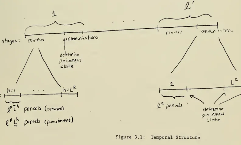
Step 2 (Temporal Structure) : We first describe the temporal structure of

the game, which consists of i' repetitions of a review stage followed by a

C R R

communications stage. Set L - N(N-2)(N-1) ! . A review stage lasts H L

C C

periods, and a communications stage lasts i L periods. Each stage is

p

further subdivided into phases; a review stage into L phases indexed by

R "' _C

19

described below. The temporal structure is outlined in Figure 3.1; the game

lasts T = 2'

(2W2^L^)

The length of a phase of a review stage depend on whether it is

rega-rded as a reward or punishment stage; if it is a reward stage, the h phase

lasts i L periods; if it is a punishment stage it lasts 2 L periods.

Q

Each phase of a communications stage lasts 2 periods.

Each communications phase is assigned an index (i,j,k) corresponding

to a triple of players. (Each index generally occurs more than once.) The

first (N-2)(N-1)! phases have indices (i,j,l); the next (N-2)(N-1)!

have indices (i,j,2), and so forth. Fixing k, the third index, the

(i,j) indices are determined by taking the set of all players but k, and

calculating every permutation of the set, giving rise to (N-1) ! blocks of

(N-2) periods. Fix a permutation, _^i •i-o _^vj t- Then the first index

in the block is (i-,i„,k); the second (i„,i„,k) and so forth up to

(i _,i , ,k) . The point of this rather complex structure is that because

n-2 n-1 "^ '^

the game is informationally connected, each player has an opportunity to

send a signal to all other players, without being blocked by any other

single player.

Using the fact that the game is informationally connected, we associate

distinct triples (i,j,k) with certain mixed strategies. If i is

connec-ted to _j despite k, we say that (i,j,k) is an active link, and let.

a -^ be the action allowing communication and _{a. the deviation for}

pla-yer i that enables him to communicate with j . If i is not connected to

j despite k we say that (i,j,k) is an inactive link, and arbitrarily

, r:.

ijk^,-l

j^ijk^,-l

define a to be a , and a.-" to be a .

Step 3 (Strategies): We now describe player i's strategy. He may be in

20

sVa^i

"

-X

/I

^

21

in the reward state. The punishment state is absorbing, so once reached,

player i rema-ins there forever. We must describe how a player plays in

each state, and when he moves from the reward to punishment state.

In the reward state and review stage, player i regards the stage as

R-h

divided into L' phases, with phase h lasting Z L periods. During the

h phase he plays a.. In the reward state and communications stage, in

i' ik

the phase indexed by (i',j,k) he plays a. -^

.

In the punishment state and review stage, player i regards the stage

R h

as subdivided into L' phases, with phase h lasting i L periods.

Dur-ing the h phase he plays q. . In the punishment state and communications

i' ik

stage, in the phase indexed by (i',j,k) he plays a. if i ?^ i' , and

he plays a. if i = i'

.

Player i can change states only at the end of a review stage, or at

the end of a communications phase (j,i,k) that is an active link. The

transition is determined by a parameter e'.

At the end of each reward phase of the review stage player i

cal-culates 7r.(z.)

₁₁

^1

occurred. If at the end of the review stage \n. (•)-it. (• ,a _)| > e' for any

h, player i switches to the punishment state.

At the end of the p communications phase corresponding to a triple

(j,i,k) that is an active link, player i calculates n.(z.) to be the

fraction of the £ periods in which z occurred. If

Itt. (•)-".(• Ia )| > e' , player i switches to the punishment state.

In all other cases player i's state does not change; in particular

the punishment state is absorbing.

R C

We must show how to choose 2' , S. , 2 and e' to give expected

22

player from deviating.

Step 4 (Payoffs): First we consider the equilibrium payoffs. Let n'

den-ote the probability that no player ever enters the punishment state and let

v' be the expected payoff vector conditional on this. Let

V = S, ., (L /L )v

. The payoff v' differs from v solely due to

communi-cations phases, yielding

r r

.

/, .x I-, -I i L d d

(4.1) |v'-v| <

A^+/l^

l+(//i^)(LV^)

where recall that d is the greatest difference between any payoffs. Since

|v-v| < e by construction, we conclude

(4.2) |w^(a)-v^| < £ + a

Ll+(iVS(LVS

+ d-TT')

R C

This shows we must take 2 /£. very large and n' close to one. We will

show that the weak law of large numbers implies that n' close to one if

R C

i and i are both sufficiently large (relative to e').

Step 5 (Gain to Deviating): Next, we consider how much a player might gain

by deviating. During a communications stage (or in any period for that

C C R R C C

matter) the greatest per period gain is d. However, only £ L /{2 L +2 L )

of the periods in the game lie in communications phases so we have the

greatest per period gain over the whole game due to deviations during

communications is

(4.3) [communications]

l+(Ji^/f)l^/lP)

Next we consider review stages. Fixing a deviator, there are three

possibilities: all other players are in the punishment state; all are in

23

contemplating deviating may not be certain which of these is true, but since

he can only benefit from this extra information, we may suppose he knows

which case he faces.

If all other players are in the punishment state they will remain there

regardless of player i's play. Regardless of how he plays during a

punishment phase, player i gets at most v.. Since |S(L /L )v. -v. | < e,

T

the largest gain over W. (a) that player i can obtain by deviating

throught the punishment state is

T

(4.4) (punishment) e + v - W.(a) <

2£ + d

Ll+(iVS(LVS

+ (l-:r')

where the inequality follows from (4.2).

Next, suppose that other players disagree about the state (so in

particular, N > 2). Then player i can possibly get d per period. Let

TT be a lower bound on the probability that all opponents agree on a

punishment state at the end of the subsequent communications stage (and

therefore agree for the rest of the game) . Then the deviating player can at

best hope to get d for one stage with probability n, and d in all

periods with probability (I-tt) . Since there are £' review phases, d

per period for one phase is actually worth d/£' yielding

(4.5) [confusion]

—

This leaves review stages where all opponents are in the reward state.

Let I-tt' be an upper bound on the probability that player i both gains

more than 2e and no opponent enters the punishment state at the end of the

24

more than 2f and remain with all opponents in the reward state next stage

with probability no more than I-tt' . Since at best he can gain d, player

i gains at most

(4.6) [reward] 2e + j;^ + (l-7r')d.

in reward stages.

Adding these bounds, we find an upper bound on the gain to deviating

(4.7) [total] r> _{^r u r} + ^^ + TT + (l-^)d +

^

l+(iV^

)lVl^

R C

Our goal is to find i'.i ,2 ,(.' to simultaneously make (4.2) and (4.6)

smaller than lOOf

.

C R

Step 6: Fix 2' so that d/2' < e. Let 2 (2 ) be the largest integer

smaller than ^2 where

1+(1/7)(lV^)

— e .

We may then simplify (4.2) to

(4.2') |wT(a)-v.| < 2e + (l-^')d,

and (4.7) to

(4.7') 8£ + (l-^)d + (l-7r')d + (l-:;^')d.

Consequently, it suffices to show that we can choose 2 and e' so that

C C R -

-when 2 - 2 {2 ) , (I-tt'), (I-tt) , (I-tt') are all less than or equal to

e/d.

By Lemma A.l in the Appendix, for the h reward phase there exists c

and 2 such that for all e' < e and 2 > 2 the probability that

25

- 1/L^

to punishment at the end of the stage is at least (1-e/d)

Consequently, for e' < min e , i > max i , we have n' > I - e/d.

By Lemma A.2 in the Appendix, for the (j,k,i) that are active

ilei ilei

communications links there exist e-' and i-^ such that for all

e' < e-^

""

and £ > i^ if player _j plays a. and players k' ?^ i

iki

play ar., the probability of k switching to punishment at the end of the

phase is at least (1-e/d) . Consequently, for e' < min e

-^

,

2 > max 2 , we have tt > 1 - e/d. Note that £ > max 2 , provided

i^ -

i^(/)

/

Fix then e' - min(e'^, e^^^) , and i* - max{i'^, (l+7)i^^ /-y) . By the

weak law of large numbers, there exists an 2** such that for

2' > i**, tt' > 1 - e/d. Choosing 2' = max{i*,^**) then completes the

proof.

Remark: How frequently does punishment occur? As T -+ «, the proof shows

that the probability of punishment goes to zero. Examining the proof of

Theorem 3.1, we see that infinite equilibria are constructed by splicing

together a sequence of truncated equilibria. For approximate discounted

equilibria, the construction repeats the same equilibrium over and over, so

that the probability of punishment in each round is constant. By the

zero-one law, this means punishment occurs infinitely often.

In the case of time average equilibria, it is irrelevant whether

punishment occurs infinitely often or not. The truncated equilibria that

are spliced together have decreasing probability of punishment, say

»r..,7r„,... -»• _0. By the zero-one _{law, if Z}

.. tt = co, punishment occurs

CO

infinitely often, while if S - tt < ", punishment almost surely stops in

26

2 tt' < 00. The corresponding truncated equilibria when spliced together

form a time average equilibrium in which punishment almost surely ceases.

On the other hand, we may form a sequence in which the t truncated

equilibrium is repeated 1/t times. Splicing this sequence together

CO

clearly yields a time-average equilibrium with S tt' - <», and so

punishment occurs infinite often.

This discussion should be contrasted with the results of Radner [1981]

in which punishment is infinitely often, and Fudenberg.Kreps and Maskin

27

APPENDIX

Proof of Lemma 4.2: We may regard Z. .M. + 1 dimensional Euclidean space

as having components tt. , j?*i and g . Define F to be the subset of this

space such that there exists a mixed strategy /i. for player 1 with

n. = 7r.(»,a.,Q .) and g. < g.(a.,a .). Let tt be the E. .M. vector

j J^ L -1 ^1 '^1 1 -L Jr^l _J

with components 7r.(',a ), and let g. - g. (a ). Then {n,g.) G F and for

A > 0, enforceability implies (7r,g.+A) F. Moreover, F is a convex

polyhedral set and its extreme points correspond to pure strategies for

player i.

Since F is convex polyhedral, we may characterize {n,g ) e F by the

linear inequalities A(7r-7r) + b(g.-g.) > c, where A is a matrix, b and

c are vectors. Consider minimizing X(n-n) - (g.-g.) subject to this

constraint. Suppose this problem has a solution equal to zero. Then

Att > g. +77 where r? - Att - _g. , and Att - g. + rj, the desired conclusion.

Since (7r,g.) G F, a feasible solution to the primal exists, so a

minimum of zero exists, if and only if the dual has a feasible plan yielding

zero. The dual is to maximize aic subject to

(cok,dh) - (A,-l)

tj > 0.

In other words, if we can find

w>0,

wc-0,

cob--l,

A — wA . is the desired solution.

Recall that (T.g.) 6 F, so > c. Moreover, if A(7r-7r) + b(g.-g.) > c

and g'. > _g. , A(7r-7r) + b(g'.-g.) > c implying that > b. Finally, for

A > 0, bA 3^ c. We conclude for some component p. c - 0, b < 0. Choose

P P

then w - q ?^ _p and w - 1. This is the desired solution. I

28

Lemma A.

1

: Suppose players ji^i are in the reward state and follow their

equilibrium strategies in review phase h. For every _P > there exists

an e and i. such that for e' < e and i ^ -?

,

Prob{3j^i|^^(-)-7r.(-,a'^)| < e' and (1/L^i^) S r.(t) > g.(a^) + 2e} < /3

J J _t=l ^ ^

regardless of the strategy used by player i. (Recall that r (t) =

r.(z.(t)) is player i's realized payoff in period t.)

Proof: From Lemma 4.2 there exist for ii^i m. -vectors of weights A. and

J J

a scalar rj such that E. .A.7r.(«,a.,Q: .) > g.(a,,a .) + r? and

J*^^ J J 1 -1 ''i 1 -1

V\ 1-1

S. .A.-7r.(',Q ) — B.(a ) + ri. Consider then the random variable

x(t) = S. .A.(z.(t)), where A.(z.(t)) is the component of z.(t)

J'^i J J J J J

corresponding to z.. The idea of this construction is to use a single

random variable x(t) to summarize the information received by all other

players. Let

L'V

S X.n^(-) " (1/L^i^) 2 x(t) = X.

j^i ^ -"

t=l

It is clear then that there exists e such that if x > g. (a ) + r? + £

then |7r.-7r.(«,Q; )| > e for some j. That is, if the sample mean x is

far from its theoretical distribution under a then some player j?^i will

observe that his empirical information tx. is far from what it would be if

J

player i had played a . Consequently, it suffices to show with

L^/

p. = 2 r.(t) that

" _t-1 ^

Prob{x < g.(a ) + r? + e and p. > g.(a ) + 2£) < 1-/9.

29

i(t) - x(t) - E[x(t)|x(t-1) r(t-l) _].

These are uncorrelated random variables with zero mean and are bounded

independent of the particular strategy of player i. Similarly

considera-tions apply to r(t) = r(t) - E[r(t) |x(t-l) , . .

.

,r(t-l) , . .

. ] . Consequently

R — —

the weak law of large numbers shows that as Z

-",

x,r->0

probabil-ity uniformly over strategies for player i. Let Q:.(t) be player i's

mixed action at t conditional on x(t-l) r(t-l) Then

E[x(t)|x(t-1) r(t-l),...] - S A TT (.,a (t),a^ ) > g (a (t),a'^ ) + r,

Js^l _{J J} 1 -1

11

- E[r(t)|x(t-1) r(t-l)....] + rj.

Consequently Prob{x

-r

x<g(a)+r7+e

r > g. (a ) + 2e implies x - r < rj - e , this gives the desired conclusion.

Lemma A.

2

: Suppose player _j is in the punishment state, and that (j,k,i)

is an active communication phase. If all players k'r'i follow their

equi-ilei. i

lei-librium strategies then for every 1 > /3 there exists an e-^ and i-"

such that for e' < e^^^ and i^ > i^^^

Prob(

I

^j.'^^

(.) - 7r^(.,aJ^^)| > £') > /3.

Proof: This is similar to, but simpler than Lemma A.l. Observe that the

iIci. ilei

set of vectors tt, = tt, (•,q-' ,a. ,a . ,) for different a. is compact

•

k k 1 -J-i i

iki

convex, and by assumption does not contain tt (•,q-' ). Consequently, we

may find a m, -vector of weights A and a scalar r; > such that Att > rj

and Att (..a-^ ^)

=0.

there exists £-' _{such that if x > r?/2}

, \t\-^ -tt. (• ,a ₎ | >

£-^ . Again

x(t) = x(t) - E[x(t) _|x(t-l) , . .

30

probability. Since E[x(t)

|x(t-l)

,...]=

)>

,7 , we

31

REFERENCES

Abreu, D., D. Pearce and E. Stacchetti (1987), "Toward a Theory of

Discounted Repeated Games With Imperfect Monitoring," unpublished ms.

,

Harvard.

, (1986), "Optimal Cartel Monitoring With Imperfect Information,"

Journal of Economic Theory. 39, 251-69.

Friedman, J. (1972), "A Non-Cooperative Equilibrium for Supergames," Review

of Economic Studies. 38, 1-12.

Fudenberg, D., D. Kreps and E. Maskin (1989), "Repeated Games With Long Run

and Short Run Players," mimeo, MIT.

Fudenberg, D., D. Levine, and E. Maskin (1989), "The Folk Theorem With

Imperfect Public Information," mimeo.

Fudenberg, D. , and E. Maskin (1986a), "Folk Theorems for Repeated Games With

Discounting and Incomplete Information," Econometrica. 54, 533-54.

(1986b), "Discounted Repeated Games With One-Sided Moral Hazard,"

unpublished ms. , MIT.

(1989) , "The Dispensability of Public Randomizations in

Discounted Repeated Games," unpublished ms. , MIT.

Fudenberg, D., and D. Levine [1983], "Subgame Perfect Equilibria of

Finite-and Infinite-Horizon Games," Journal of Economic Theory. 31 (December),

251-63.

Green, E. , and R. Porter (1984), "Noncooperative Collusion Under Imperfect

Price Information," Econometrica. 52, 87-100.

Kreps, D. , and R. Wilson (1982), "Sequential Equilibrium," Econometrica. 50,

32

Lehrer, E. (1985), "Two-Player Repeated Games With Non-Observable Actions

and Observable Payoffs," mimeo, Northwestern.

(1988a) , "Extensions of the Folk Theorem to Games With Imperfect

Monitoring," mimeo, Northwestern.

(1988b), "Internal Correlation in Repeated Games," Northwestern,

CMSEMS Discussion Paper #800.

(1988c), "Nash Equilibria of n-Player Repeated Games With

Semi-Standard Information," mimeo, Northwestern.

(1988d), "Two Players' Repeated Games With Non-Observable

Actions," mimeo, Northwestern.

(1989) , "Lower Equilibrium Payoffs in Two-Players Repeated Games

With Nonobservable Actions," forthcoming, International Journal of Game

Theory.

Porter, R. (1983), "Optimal Cartel Trigger-Price Strategies," Journal of

Economic Theory. 29, 313-38.

Radner, R. (1981), "Monitoring Cooperative Agreements in a Repeated

Principal-Agent Relationship," Econometrica. 49, 1127-48.

(1985), "Repeated Principal Agent Games With Discounting,"

Econometrica. 53, 1173-98.

(1986) , "Repeated Partnership Games With Imperfect Monitoring and

No Discounting," Review of Economic Studies. 53, 43-58.

Radner, R. ,' _{R. Myerson and}

E. Maskin (1986), "An Example of a Repeated

Partnership Game With Discounting and With Uniformly Inefficient

Equilibria," Review of Economic Studies. 53, 59-70.

Rubinstein, A. and M. Yaari (1983), "Repeated Insurance Contracts and Moral

33

Sorin, S. (1988), "Asymptotic Properties of a Non-Zero Sum Stochastic Game,"

International Journal of Game Theory. 15, 101-107.

(1986), "Supergames," mimeo, CORE.

Stigler, G. (1961), "The Economics of Information," Journal of Political

Date

Due

24

m\

MIT LIBRARIES DUPL I