Identifying indicators of the spatial variations of agricultural practices by a tree partitioning methods: the case of weed control practices in vine growing catchment

HAL Id: hal-00454525

https://hal.archives-ouvertes.fr/hal-00454525

HAL is a multi-disciplinary open access

archive for the deposit and dissemination of sci-entific research documents, whether they are pub-lished or not. The documents may come from teaching and research institutions in France or abroad, or from public or private research centers.

L’archive ouverte pluridisciplinaire HAL, est destinée au dépôt et à la diffusion de documents scientifiques de niveau recherche, publiés ou non, émanant des établissements d’enseignement et de recherche français ou étrangers, des laboratoires publics ou privés.

agricultural practices by a tree partitioning methods:

the case of weed control practices in vine growing

catchment

Anne Biarnès, Jean-Stéphane Bailly, Y. Boissieux

To cite this version:

Anne Biarnès, Jean-Stéphane Bailly, Y. Boissieux. Identifying indicators of the spatial variations of agricultural practices by a tree partitioning methods: the case of weed control practices in vine growing catchment. Agricultural Systems, Elsevier Masson, 2009, p. 105 - p. 116. �10.1016/j.agsy.2008.10.002�. �hal-00454525�

Identifying indicators of the spatial variation of agricultural practices by a tree partitioning method: the case of weed control practices in a vine growing catchment

A. Biarnès*, J.S. Bailly** & Y. Boissieux*

* IRD, UMR LISAH, 2 place Viala, 34090 Montpellier, France

** ENGREF-AgroParistech, UMR LISAH & TETIS, 2 place Viala, 34090 Montpellier, France

Corresponding author : Anne Biarnès Tel: +33 4 99 61 22 62

biarnes@supagro.inra.fr

Abstract:

Environmental impact assessments of agricultural practices on a regional scale may be computed by running spatially distributed biophysical models using mapped input data on agricultural practices. In cases of hydrological impact assessments, such as herbicide pollution through run-off, methods for generating these data over the entire water resource catchment and at the plot resolution are needed. In this study, we aimed to identify indicators for simulating the spatial distribution of weed control practices (WCP) in a French vine growing catchment. On the basis of interviews of 63 winegrowers, a spatially explicit database was developed that included 1007 vine plots and information regarding practices and potential explanatory variables. Four practices were differentiated according to the methods used (chemical weed control, shallow tillage, grass cover or a combination) that determine the intensity of herbicide use and potential surface run-off. Three groups of explanatory variables corresponding to three assumed levels of spatial organisation of WCP (the plot, the farm and the local government area (LGA)) were tested and compared. In the first step, selection of explanatory variables within each group was performed using a tree-partitioning method that combined the advantages of the CART algorithm (building an interpretable and controlled model) and the Random Forest algorithm (limiting overfitting) algorithm. In the second step, the performance of the selected variables for reproducing the observed repartition of practices was evaluated by a stochastic use of the tree, leading to a set of equiprobable spatial distributions of practices at the plot resolution. The results indicate that plot characteristics related to alley width play an important role in the weed control choices; however, to take into account the total diversity of the WCP, it appears to be necessary to focus on the farm holding variables and, in particular, on the variable LGA. However, the interpretation of these results is still difficult. Specifically, the great relevance of the variable LGA to discriminate the practices may be related to various factors, one of which is the distribution of soil properties within the Peyne catchment that still requires more precise characterization. The results also indicate that the combination of the three groups of variables leads to the highest-performing simulations of the spatial distribution of WCP. Nevertheless, the farm holding variables provided little additional spatial information, which supports the idea that they may be omitted without significantly impacting the final results.

Keywords: Viticulture, classification tree, uncertainties, stochastic simulation, indicators of practices

1. Introduction

Since land use is an important factor in governing environmental impacts (see for example, Ojima et al., 1994; Thapa and Rasul, 2005), new challenges for agriculture are emerging from societal requirements for sustainable development, such as preservation of water resources, soil conservation, and gene flow restriction within cultivated landscapes.

Proper solutions to these new challenges require environmental impact assessments of agricultural practices at the regional scale. In many environmental cases, these assessments are computed by running spatially distributed biophysical models that require large amounts of mapped input data (Faivre et al., 2004), including data on agricultural practices. The extension and spatial resolution of the data on agricultural practices must be appropriately scaled to the underlying biophysical process being modelled. For instance, in the case of regional water resources assessments, the water fluxes that have to be considered are mainly vertical (e.g., Leenhardt et al., 2004). Thus, only knowledge of the global spatial trends of practice distributions is necessary. Spatial resolution of data on agricultural practice can be coarse (small agricultural area, local government area) and simply correspond to an estimation of the proportion of each practice. But in cases where the hydrological processes are also significantly governed by lateral flow there is a need to map agricultural practices over the entire water resource catchment at plot resolution. Indeed, spatial plot design induces spatial practice discontinuities that impact lateral water flows. Therefore, the precise location of agricultural practices in the catchment can be important for assessing environmental impacts on water resources, for example regarding nitrogen fluxes (Beaujouan et al., 2001).

Since existing agricultural inventories generally do not provide data on practices at field resolution, methods that aim to map variability of agricultural practices need to be proposed. For large areas with numerous farmers, exhaustive ground surveys or enquiries are clearly unrealistic. Therefore, an approach is to invest in spatial observation techniques, such as remote sensing. Even though remote sensing has proven value for mapping land use, particularly for crop mapping (Faivre et al., 2004), in the process of downscaling land use from crops to agricultural practices, limitations of remote sensing are usually experienced, especially for perennial crops. For instance, remote sensing has been successfully used to map tillage practices in annual crops in the United States (e.g., Briclemeyer et al., 2006; Gowda et al., 2001; South et al., 2004); yet for perennial crops like vines, which exhibit a wider range of practices, remote sensing still appears to be ineffective for characterizing weed control practices (Wassenar et al., 2005; Corban, 2006). Moreover, remote sensing can only provide partial knowledge of practices because some technical options, particularly those involving the use of pesticides, cannot be detected.

Another strategy is to look for available spatial variables that might be used as indicators to simulate the spatial distribution of agricultural practices. It is known that agricultural practices are generally not randomly distributed in space, since they result from spatially structured driving factors (Verburg et al. 1999; Thapa and Rasul, 2005). Agricultural practices can therefore be predicted after (1) identifying the set of spatially explicit indicators that correspond to agricultural driving factors, and (2) assessing the statistical relations between these factors and the practices. Such methods, which are usually based on multivariate statistical analysis, use data from censuses, remote sensing, maps, and enquiries. Geographers and agronomists have already developed such methods at various scales of resolution, including the field scale, both to map current or future land use and to assess the relative importance of socio-economical and biophysical factors on the spatial

distribution of land use (e.g., Pierret, 1996; Verburg et al., 1999; Veldkamp and Lambin, 2001; Veldkamp and Verburg, 2004). However, these studies have dealt primarily with a definition of land use that is restricted to the specification of land use (cultivated area, forest, grassland, etc.), to the main crop groups (annual vs. permanent crop) and sometimes to crop types (wheat, maize, etc.) Details on crop management systems are often omitted from these methods. When such information is required, most studies are based not on an indicator approach, but on the use of averaged data derived from the literature, experts' assessments, technical recommendations (e.g., Giupponi et al., 1999; Mignolet et al., 2004) or the use of schemes with a uniform spatial distribution of agricultural practices (e.g., Knox et al., 1996; Hartkamp et al., 2004). In contrast, the few studies based on a search of spatialized indicators to map crop management systems have not been not applied at plot resolution but rather at coarser resolutions (Maton et al., 2007).

The objective of this paper was to identify indicators that are suitable to simulate the spatial distribution of agricultural practices on a water resource catchment at plot resolution. This paper is based on the specific case of weed control practices in a vine growing catchment in southern France. Section two presents the study area, the data and the statistical and probabilistic (i.e., stochastic) approaches used. The method used represents an extension of the classical CART segmentation algorithm. Three groups of potential explanatory variables were tested and compared. These three groups correspond to three assumed levels of the spatial organisation of weed control practices. The results are presented and discussed in sections three and four.

2. Materials and Methods 2.1. Study site

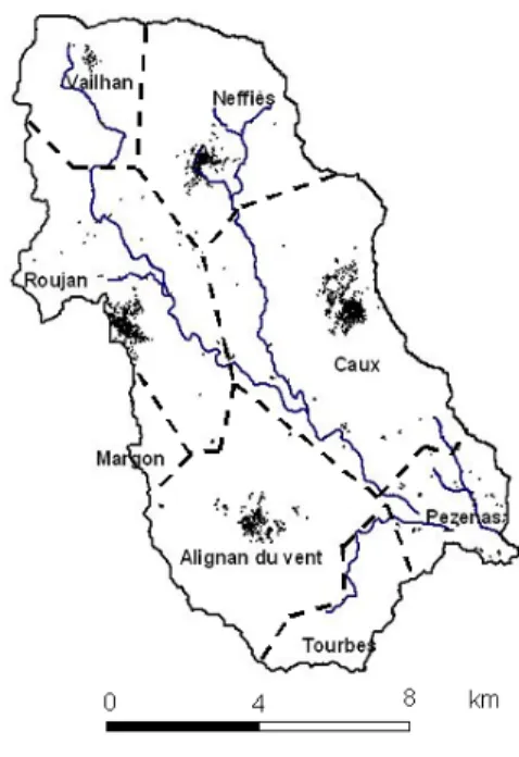
We studied the Peyne river catchment in the mid Hérault valley in the Languedoc-Roussillon region of France, one of the world’s largest wine-producing regions (Figure 1). This catchment suffers from serious herbicide pollution of the surface water. Studies show that this pollution is related to herbicide leaching through runoff during heavy rainfall that is typical of the area’s sub-humid Mediterranean climate (Lennartz et al., 1997; Louchard et al., 2001). Vineyard weed control practices play a crucial role, since they determine both the type and amount of herbicide applied and the evolution of soil surface characteristics on which surface runoff depends (Leonard and Andrieux, 1998; Hébrard et al., 2006). The Peyne river catchment is a representative example of a vineyard catchment in the mid Hérault valley, both in terms of physical characteristics and land use. It covers 75 km², about the same size as catchments in the region that are used as water resources and the area includes about 5000 ha of vines. It presents a succession of clearly differentiated geomorphological units that strongly determine the distribution of soils within the landscape (Bonfils, 1993). The region’s altitude ranges from 20 m (southeast of the catchment) to 340 m (northwest of the catchment). There are sharp contrasts in landscape between the northwest, which is rugged and mainly scrub-covered with little arable land, and the rest of the valley, which has gentler landforms and is almost entirely covered by vines.

The Peyne catchment incorporates all or part of the territories of eight local government areas (LGA, in France referred to as “communes”) and is farmed by 650 winegrowers. In 2000, according to data from the last farm census carried out by the Regional Direction of Agriculture and Forest, 61% of the farm holdings of the LGAs of the catchment cultivated under 5 ha of vines, and only 6% over 20 ha. In terms of area, the former represented only

12% of the vineyard area, whereas the latter represented 26%. 93% of the holdings supplied their grapes to cooperative wineries, whereas the others use private wineries. Four mono-LGA-based cooperative wineries (those of Alignan du vent, Margon, Roujan and Tourbes) and two bi-LGAs-based cooperative wineries (those of Vailhan-Neffiès and of Caux-Pezenas) collect most of the grape production. In the case of the mono-LGA-based cooperative wineries, the supply basin of each winery extends over a great part of the vine growing area of the LGA where the winery is located. In the case of the other two wineries of the Peyne catchment, the supply basin of each winery also includes the neighbouring LGA.

2.2. Data

A geographical database was developed that included (a) information regarding weed control practices (WCP) and (b) a description of physical or socio-economic variables that can potentially explain the practices. The database included a sample of 1007 geo-referenced vine plots of land that are owned by 63 winegrowers.

2.2.1. Sampling scheme and data collection

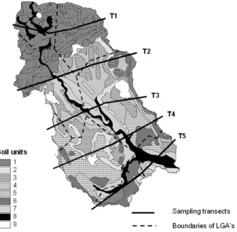
The required data were gathered by surveying winegrowers. The winegrowers were selected by sampling vine plots along five transects perpendicular to the Peyne river. The transects were regularly spread from upstream to downstream so as to intersect LGAs, soil and geomorphological units (Figure 2). Along each transect, one-fifth of the vine plots were randomly selected. The winegrowers cultivating these plots were contacted by telephone in order to make an appointment for the inquiries, which were conducted at the winegrowers’ residences. The refusal rate was 8%. Sixty-three winegrowers were surveyed. These winegrowers cultivated a total of 1007 vine plots within the Peyne catchment, i.e., about 20% of the area under vines within the Peyne valley. Due to the unequal repartition of the farm holdings structures, such sampling gave more weight to the larger farms. We assumed that this sampling was representative of the spatial weight of the farms and of the distribution of WCP in the catchment.

The survey questionnaire consisted of two parts. The first focused on the WCP used in each plot cultivated by the selected winegrowers. The second part was designed to provide data for the variables that were assumed to explain the choice of practices. In addition, the plots were precisely located on both the land register map and the 1:100,000 soil map of Bonfils (1993).

2.2.2. Weed control practices

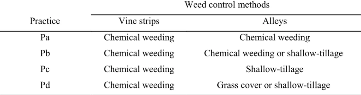
From the collected data, a 4-type expert-based classification of the WCP was performed. The types were distinguished according to: (1) their potential impact on soil surface features and surface runoff, characterised by a range of different possible soil surface characteristics during the year and their corresponding infiltration values, and (2) their intensity of herbicide use, characterised by the mean amount of herbicide used per year. As shown in Table 1, the practices differed in the weed control methods used in the alleys and the vine strips. Practice Pa was based on chemical weeding in vine strips and alleys alike. The other three practices, Pb, Pc, and Pd also used chemical weeding in the strips, but differed in the methods used for the alleys. In practice Pc, the alleys were repeatedly shallow-tilled. Practices Pb and Pd both managed some alleys by shallow tillage but alternated these at regular intervals within the plot with alleys managed by a different method. In practice Pb, shallow tillage alternated with chemical weed control, and in Pd, shallow tillage alternated with alleys under permanent grass, natural or sown and

controlled by mower or rotary cutter. In both Pb and Pd, the untilled alleys were those where tractors passed to spray pesticides during the spring and summer; shallow tilling was not used so as to ensure a good load-bearing capacity. In the case of Pd, the use of grass cover also aimed to reduce vine vigor and production through competition for water and mineral nutriments. This practice may be necessary when plot yield is over the threshold authorized by the French wine legislation, for example.

As a trend, these practices can be ranked according to the risk of runoff and herbicide leaching they generate. From Pa to Pd (Pa > Pb >Pc > Pd), the environmental risk decreases due to a reduction of herbicide used (from total to partial chemical weed control) and to the use of weed control methods that reduce surface runoff.

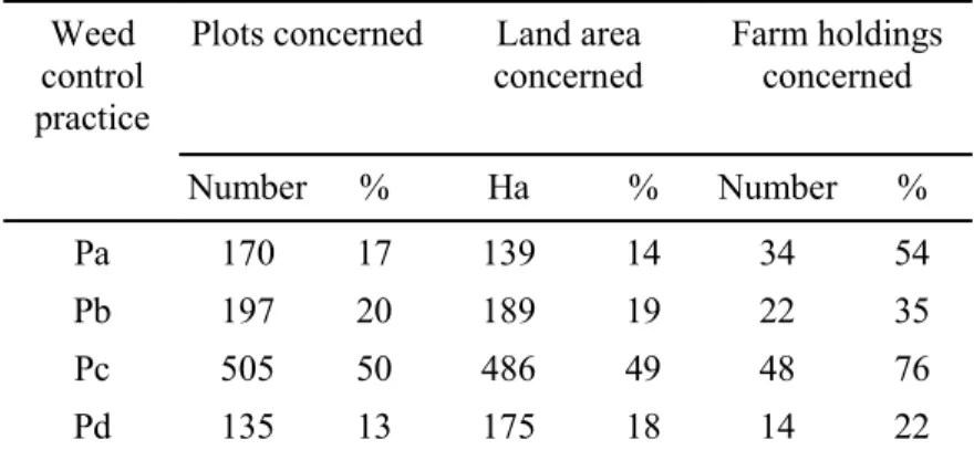
The survey results are summarized in Table 2. They show that the most common practice, Pc, was used on 50% of vine plots, 49% of the land area concerned and by 76% of the winegrowers interviewed. A majority of winegrowers (54%) also used practice Pa, but on fewer plots (17%) and on a much smaller land area (14%). Practices Pb and Pd were used by a minority of winegrowers, and both were used on about the same number of plots and the same area as Pa.

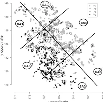
The location of each type of practice in space according to the geographic coordinates of the surveyed plot centroids clearly shows that the WCP were not randomly distributed in space (Figure 3). Pc was the dominant practice in plots located on the left side of the Peyne river (east-northeast side); whereas Pb and Pd were dominant in plots located on the right side of the river (west-southwest side).

2.2.3. Potential explanatory variables

In order to further extend the use of identified explanatory variables to simulate the spatial distribution of WCP throughout the whole Peyne catchment or other vineyard areas of the region, we collected variables that (1) we assumed to be potentially explanatory of the WCP and (2) which were directly (or assumed to be indirectly) available at plot scale from digital regional maps, very high spatial resolution images from French Geographic Mapping Agency (IGN) and national databases.

The collected potential explanatory variables belonged to three groups corresponding to three hypothesized levels of spatial organisation of practice diversity and different degrees of direct availability at plot scale: (1) the physical characteristics of the plots; (2) the structural characteristics and production priorities of the farm holdings; and (3) the local government area (LGA) the plots belong to.

Concerning the spatial organisation of practices, the choice of these three groups of variables was guided (1) by the agronomic literature, which emphasizes the plot and the farm levels to explain the diversity of practices at local or regional scale (Gras et al., 1989; Dounias et al., 1998; Maton et al., 2007) and (2) by the results of a previous study conducted in two of the eight LGAs of the valley, in which the authors confirmed the influence of plot and farm levels (in the case of WCP) and suggested an effect at the LGA level (Biarnès et al., 2004).

Concerning the availability of variables, the variables of the plot and LGA groups can be collected directly at the plot scale by remote sensing (Delenne et al., 2008) and regional digital maps. The farm holding variables are nor directly available at the plot scale. They are usually aggregated at the LGA scale in national databases. To obtain them at the plot scale, without any exhaustive inquiries, a procedure needs to be developed to allocate plots to farm holdings. Although attempts to better geo-reference farm holding territories can be

found in the literature (e.g. Durr and Froggatt, 2002), no procedure has been proposed to produce explicit farm territories defined at the plot resolution.

a- The plot physical characteristics variables

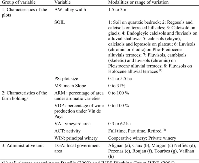
The plot physical characteristics variables (Table 3) were intended to take into account four specific constraints of the plots that might limit the technical options: the type of soil (SOIL), the mean slope (MS), the size of the plot (SP), and the alley width (AW). These variables are respectively available from the regional soil map, DEM (digital elevation model from IGN©) and remote sensing (Delenne et al., 2008).

The soils of the Peyne catchment present contrasting characteristics of moisture and surface texture that determine their mechanical properties (bearing capacity, crusting sensibility) and which might therefore influence the choice of weed control practices. The only available regional map was the 1/100,000 map by Bonfils (1993), which differentiates the soil units according to landscape units. In order to reduce the number of soil units, particularly in the northern part of the catchment where there are very few vine plots, we created an expert-based reclassification of the soils of this map. Eight units of soil (better reflecting landscape units than the original map) were differentiated (Table 3 and Figure 2).

The mean slopes and the sizes of the plots varied respectively from 0 to 31 % and from 0.3 ha to 5.5 ha. A high slope or small plot size make tractor use difficult.

Vine spacing varied greatly, with alley widths ranging from 1.5 m to 3 m. This heterogeneity results from the gradual replanting associated with mechanization since the 1960s, and from the switch from mass production of Vin de Table to quality wines (Appellation d’origine contrôlée or Vin de Pays) since the 1970s. Alley width determines both the maximum size of equipment that can pass in the alleys and the ease of work. Only equipment under 1 m wide can be used if the alley width is 1.6 m or less. Such widths are suitable for animal traction, but make it difficult for tractors to pass easily.

b- The farm holding characteristics variables

Ten variables characterizing the farm holdings were collected : “cultivated area of the holding” (CA); “vineyard area of the holding” (VA); “mean age of the vineyard” (MAV); “percentage of the vineyard area under aromatic varieties” (ARM); “percentage of wine production under Vin de Pays” (VDP), “under Appellation d’origine contrôlée” (AOC), “under Vin de Table” (VDP); “principal winery of the farm holding” (WIN); total manpower (TMP), “other activity” (ACT). These variables are commonly used to characterize the diversity of the winegrowing farms in the Languedoc-Roussillon (Agreste, 1996; Agreste, 2001). They are all available in national administrative farm census databases. We did not collect information on the characteristics of the weed control equipment because such information is not available in farm census databases. From the collected variables, only five independent variables were kept: VA, ARM, VDP, ACT, WIN for the analysis presented in this paper (Table 3). The other variables were left out due to their correlations with these five variables. For each variable, an identical value was attributed to all sets of plots belonging to the same farm holding.

c – The LGA variable

The third group of variables only had one variable, “the local government area the plot belongs to” (LGA), which is available from an administrative map. In the Peyne catchment, such a variable may be considered as a proxy of the local government area to which the farm belongs because most farm holdings have a majority of their plots within

the local government area where they are based. This variable was intended to take into account the natural and socio-professional environment of the winegrowers, including relations between neighbours and the influence of the LGAs-based cooperative wineries in the organization of the industry.

d- Correlation between groups

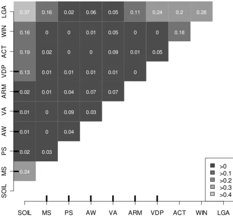
In order to analyse the independence of these three groups of variables, in Figure 4 we computed: the determination coefficient when crossing two numerical variables; the Cramer statistic, derived from the chi-square test used when crossing two qualitative variables; and the eta-square statistic, derived from the ANOVA sum of variances when crossing a qualitative variable and a numerical one. All of these statistics can be interpreted in the same way: values close to zero indicate independent variables; values close to one indicate correlated variables. The results show that the three groups of variables are not entirely independent. The plot variable SOIL and the holding variables VDP, WIN and ACT are not randomly distributed among LGAs. The variable SOIL is the variable most correlated to the variable LGA, a fact that is explained by distribution of the soils within the landscapes (Figure 2). In the case of VDP, the correlation may be explained by the characteristics of the wine industry. The productive orientation of the winegrowing farm holdings is strongly determined by national regulations on wine production that delimit specific geographic areas for producing AOC or VDP wines. The Peyne valley is a VDP production area, but an AOC production area is localized in the northwest area of the valley and corresponds to part of the territory of three LGAs. The winegrowers of these LGAs that have some plots localized in this area can therefore reduce their VDP production to produce AOC wines. However, when the winegrowers are cooperative winegrowers, their productive orientations also depend on the LGA-based wineries of which they are members and, consequently, are linked to the LGA that they belong to. 2.3. Data processing

In order to optimise the choice of indicators used to reproduce the spatial distribution of agricultural practices at plot resolution, we developed methods that permit comparison of results coming from several sets of potential explanatory variables (Bailly et al., 2008). This methodological development was performed in two steps.

In the first step, a statistical modelling method based on the classification and regression tree (CART) algorithm (Breiman et al, 1984) was proposed. Rather than maximising predictive performances of the model, the method, called the robust classification tree (RCT), was built in order to obtain an explicative model, with explicative rules that can be easily interpreted and generalized in other contexts. However, at the end of this first step, the WCP classical prediction performances obtained with the proposed RCT model were compared to the model obtained with classical CART and another CART derivative algorithm in order to verify that the predictive power of the proposed method was not far away from other usual methods.

In the second step, the performance of various sets of explanatory variables to reproduce the observed repartition of practices in space was assessed by a stochastic use of the RCT. In contrast to the usual spatial prediction method that yields only a solution that minimizes prediction error, we preferred to devise a process that shows spatial uncertainties through a set of equiprobable spatial distributions of practices at plot resolution.

2.3.1. Characterisation of the stable relationships between the weed control practices and explanatory variables through the robust classification tree method

The method used is an extension of the classical CART segmentation algorithm. The CART algorithm is based on a recursive partitioning process of the multidimensional space defined by a set of explanatory variables in areas that are as homogeneous as possible regarding the variable being explained (the WCP class, in our case). The result is a binary hierarchical tree. The tree is characterised by several splits whose nodes depend on homogeneity measures (the Gini index (Gini, 1912) in our case), which determine a set of logical if-then conditions linking the variable to be explained to the explanatory variables. The branch lengths are related to the discriminating power of the splitting variables. The growth of the tree is performed on a set of samples, called the growing set. To limit overfitting, the tree is then pruned by maximizing a cost-complexity criterion measured when using the tree to predict classes on another set of samples called test set. At the end of the process, each terminal node of the tree, called a leaf, contains a probabilities vector for each class of WCP. The values of this probabilities vector are adding up to one. In a classical classification use, the major class is attributed to each leaf (Breiman et al., 1984). CART is very popular since it facilitates classification model interpretation and does not assume a particular shape (such as a linear shape) for relationships between variables. It has been widely applied over the last 20 years in many different studies, for example in landscape research (Gellrich et al., 2008) and agronomy (Tittonell et al., 2008; Maton et al., 2007). However, CART is known to be sampling-sensitive, especially when correlations between explanatory variables exist, which can be the case in the present study when using jointly the groups of explanatory variables. To overcome this problem, numerous derivative methods have been proposed (Breiman, 1996; Breiman, 2001; Geurts et al., 2006), which are all based on aggregation of several classification trees (a forest) built with randomisation. Unfortunately, if these derivative methods smooth sampling effects, the advantages of CART interpretation to obtain an easily interpretable explicative model are lost. Therefore, we developed the robust classification tree process in order to preserve the advantage of CART and the advantage of randomised tree algorithms.

The robust classification tree algorithm runs in two steps. We first built a “forest,” i.e., a collection of numerous trees (1000 trees) using random resampling without replacement, where each tree of the forest is grown on a random sample of 702 plots and pruned from the 305 others using a typical pruning process (Breiman et al.,1984). The common tree structure of the forest (the robust structure) is then extracted with a frequency analysis of the tree collection: (1) only nodes in the forest tree having the same position with the same rule for splitting for at least f% (frequency parameter) of forest trees are kept; and (2) only leaves having plots coming from at least p different farm holdings (farm parameter) are kept. To detail the former splitting rule criteria, the frequencies of each variable name and values pair are computed when the variable used for splitting is qualitative; when the variable is continuous, only frequencies of the variable name and sign pair are computed, and pairs are associated with the median continuous value.

2.3.2. Weed control practices spatial distribution simulation: comparison of explanatory variables performances

We used three sets of explanatory variables in order to assess the benefit of using the farm holding characteristics variables: set 1 contains the five farm holding characteristics variables; set 2 contains the four plot characteristics variables and the variable LGA; and set 3 contains the three groups of variables. This choice leads to three different robust trees.

a. Weed control practices prediction overall accuracy

A K-fold cross validation test was computed on each classification method (K=20) to achieve a prediction performance comparison between the proposed robust classification tree and the other classification methods. For each of the 20 loops of the test, 19/20th _{of the} 1007 plots were used to build the models (robust classification tree, CART, random forest). These models were therefore used to predict WCP on the other 1/20th

of the 1007 plots. To calculate prediction accuracy, we computed omissions and commissions on this same set of 1/20th _{of 1007 plots. The predictions were performed with a classical use of the methods} (i.e. attributing the major class of WCP to each leaf). For each new loop, the next 1/20th

of the 1007 plots were used to compute the prediction accuracy resulting from models built on the other 19/20th _{plots and so on to the end. At the end, for each classification method,} we computed a global overall accuracy coming from the arithmetic mean of the 20 accuracy rates.

b. Weed control practices spatial predictions

Each robust tree was used to predict a practice for each of the 1007 plots of the surveyed sample. For each plot, the path in the considered robust tree ends on a leaf. Since this leaf contains a probabilities vector for WCP, a WCP was thus randomly attributed to this plot with respect to the probabilities vector of the leaf. All plots were thus processed, simulating a WCP spatial distribution that was mapped using plot centroids.

c. Spatial predictions comparison

For each robust tree, a set of simulated WCP spatial distributions were compared to the observed one, dividing the whole catchment into regular sub-areas (Figure 3). For each sub-area, we computed a dissimilarity between n simulated WCP (n= 1000), giving an n by p matrix X(n), and the observed WCP distribution y = [y1, ...,yp], with y1 denoting the proportion of practice with modality 1 for instance, and p denoting the total number of modalities (p= 4). The matrix X(n) concatenates n vectors Xi (i=1,...,n) that compute for the simulation i, the proportion of plots for each practice: Xi=[X1i, ...,Xpi]. To compare a value to a distribution, the typical practices are to measure the dissimilarity using normalized Euclidean distances or methods that score when the value fails into confidence intervals for various probabilities (Goovaerts, 2001). Since we obtained correlated data ([X1i, ...,Xpi] summing to one), we preferred to compute the dissimilarity between y and X(n) for each cell using the Mahalanobis distance (Mahalanobis, 1936) given by:

d(y,X(n)) = [ (y-µ)t . Σ-1 . (y-µ) ]0.5

with : µ = [µ1, ...,µp], means of X(n) Σ = covariance matrix of X

t just denotes the transpose of the (y-µ) vector

Finally, we computed a global dissimilarity (dissimilarity between the simulated and the observed WCP distributions) for the entire catchment using a weighted average of the dissimilarities computed for each cell, with weights equal to the plot number for each cell (or sub-area).

From the previous process, we obtained a single value of global dissimilarity. In order to compare the value obtained for each robust tree, we computed a dissimilarities distribution just by repeating the previous process m times, giving m global dissimilarities for robust tree (m = 50). This allowed us to compute and empirically test the significance in the difference of dissimilarities obtained with the three sets of explanatory variables, by simply comparing the obtained distributions (comparison of the mean values and bilateral confidence intervals).

All of these methods were conducted on R 2.6.0 statistical software (Ihaka and Gentleman, 1996) using the tree package (Ripley, 2007), the Random Forest package (Liaw and Wiener, 2008) and many custom R scripts.

3. Results

3.1. Predicting the weed control practices by different sets of explanatory variables

Three robust trees (T1, T2 and T3) were obtained (Figure 5) from the three tested sets of explanatory variables with parameters f=50% (frequency parameter), p=4 (farm parameter) and from forests of 1000 trees. The three trees confirm that it is possible to find indicators of WCP distributions in each group of variables.

From the five variables tested to construct tree T1, only three variables (VDP, VA, ARM) related to the economic scale, and the productive choices of the farm holdings were kept to differentiate distributions of practices. The right branch of tree T1 is associated with VDP oriented farm holdings (percentage of wine under VDP greater than 84.5% of the total production). In these holdings, choices of practices vary according to the vine area. As a trend, winegrowers adopt practices that increasingly limit polluting runoff (Pb, then Pc, then Pd) when increasing the vine area. In the farm holdings characterized by weaker production of VDP (left branch of the tree), choices of weed control practices are linked to the percentage of area under aromatic varieties (ARM). The plots belonging to farm holdings with little renewal of their varieties (ARM <39.345% of the total vine area) are associated with intensive use of herbicide (practice Pa in 54% of the plots), which may be explained by the high proportion of vines with very small alley widths in these farm holdings. The other plots are associated with shallow tillage (Pc in 88 or 66% of the plots). The bases of trees T2 and T3 are very similar. Regarding the branch lengths, the LGA variable clearly appears to be the most discriminant. In the two trees, the root node is split based on the values of the LGA variable, dividing all the sets of plots into two groups respectively located in the LGAs on the left side (right branch of the tree) and on the right side (left branch of the tree) of the Peyne river. As a result, the trees reproduce the non-uniform distribution of practices between the two river sides and highlight its structuring effect in the spatial distribution of the practices. In opposition to our hypothesis, the variables SOIL, SP and MS do not participate in the splitting of these two groups of plots. They do not appear to be determinant criteria to discriminate the practices at the plot scale. In contrast, as hypothesised, the alley width (AW) does appear to be a discriminatory variable.

In T2, the plots characterised by narrow alleys (less than 1.75 m or than 1.875m according to the river side), are associated with intensive use of herbicide (Pa, and even Pb), which is not the case for the plots characterized by wider alleys. On the left river side, the plots with wide alleys are associated with practice Pc in 78% of the cases. On the right river side, they are almost equally associated with practices Pb, Pc or Pd.

In tree T3, in addition to the variables used by tree T2, two farm holding variables (VA and ARM) were used to differentiate the distribution of practices. These variables operate in the last nodes, after the variables LGA and AW. The most appreciable effect of these variables was in obtaining purer leaves, as for example leaf L4, which was principally associated with grass cover (Pd). This leaf contains the plots belonging to farm holdings with more than 45.175 ha of vines. The variable VDP was not used in tree T3, which suggests that due to its non-uniform distribution among LGAs, it does not provide supplementary information to better discriminate between the practices.

3.2. Prediction accuracy comparison

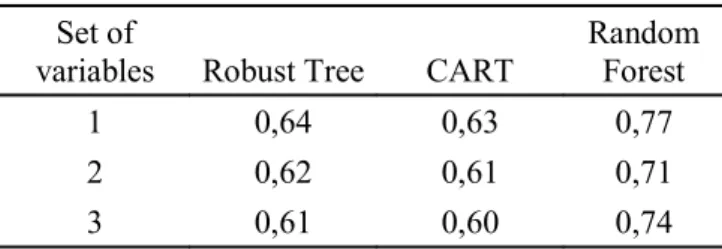
As explained in section 2.3.2, we computed a 20-fold validation test using successively robust trees, CART usual trees and random forest algorithm. The results are tabulated in Table 4 using the three sets of explanatory variables. These results show that random forest gives higher prediction accuracies and that robust trees give slightly higher accuracies than usual CART. The results also indicate that the prediction accuracy is very similar between the three tested sets of variables.

3.3. Simulating the spatial distribution of the weed control practices by the selected robust trees

Figure 6 shows four examples of simulated WCP spatial distributions: a totally random spatial simulation respecting only global practices percentages (Figure 6a) and three spatial simulations using, respectively, trees T1, T2 and T3 (Figures 6b, c and d). These examples show that a random spatial distribution looks very different from the observed one (Figure 3). Conversely, the use of spatialized indicators gives contrasting and realistic distributions between the two sides of the Peyne river. Nevertheless, these distributions are difficult to compare visually.

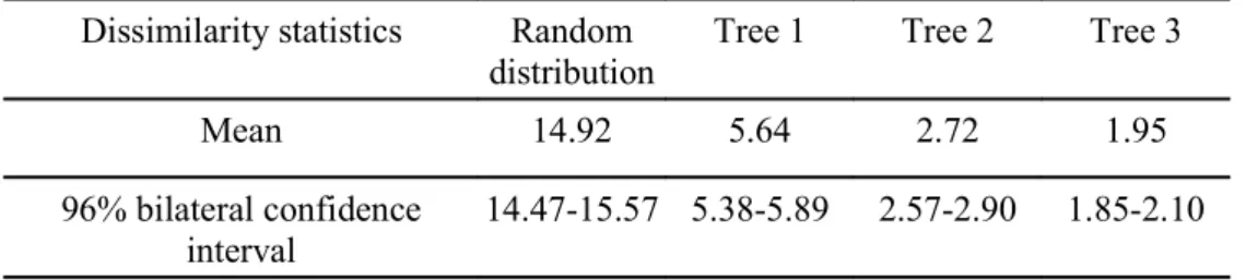
Global dissimilarities between the observed WCP distributions and 1000 simulations were first computed as explained above. This was done successively using trees T1, T2, T3 and a totally random spatial simulation. The results, presented in Table 5, confirm that simulations conditioned by trees are much better than random ones. They also show that simulations resulting from trees T2 and T3 are close but significantly different and that they are the closest to the observed distribution.

4. Discussion

4.1. Variability in weed control practices driving forces

For each of the three assumed levels of spatial organisation of practices, at least one indicator was found.

At the plot scale, the plot characteristic related to alley width explained the most important part of the distribution of practices between integral (Pa) and partial chemical weed control practices (Pb, Pc and Pd), as shown in trees T2 and T3 (Figure 5). But choosing between partial weed control practices could not be explained by this variable. In addition, the soil on a 1/100,000 map did not participate in WCP discrimination. This result may be explained by (1) the uncertainty related to the location of plots on a 1/100,000 scale soil map, (2) by the variability of soil characteristics within a soil unit. The 1/100,000 scale map is probably not sufficiently detailed to detect a relationship between soil and practices. Finally, neither the MS nor the SP variable explained the diversity of WCP, which may be

related to the small number of plots characterized by problematic values for these variables (high slopes or very small plots), since these values determine the plots that are currently abandoned by the winegrowers.

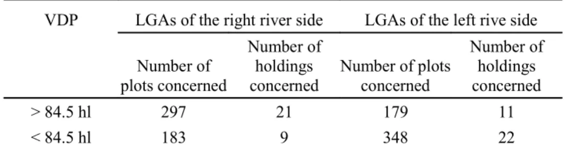
To take fullest account of the diversity of the weed control practices (Pa, Pb, Pc and Pd) and to precisely discriminate them, it appeared necessary to focus on the farm holding variables (tree T1) or to add them into the set of tested variables (tree T3). These results show that the plot constraints were not absolute, and that practice choices are handled in the farm holding context. They confirm previous studies on two Peyne catchment local government areas (Biarnès et al., 2004). From the three explanatory variables selected by the tree, ARM may be related to specific constraints of the holdings, such as the proportion of vines with very small alley widths (tree T1); VA may be related to the economic scale of the farming and an effort to adopt more environmentally-friendly practices when this economic scale increases (trees T1 and T3). However, in tree T1, the effect of VDP is difficult to interpret since this variable is correlated to the LGA variable (Figure 4). An additional independence test (chi-square test) showed that the values of VDP inferior or superior to the threshold value of tree T1 (84.5%) are unequally distributed between the left and the right river sides of the Peyne catchment (Table 6).

Lastly, by affecting the environment of the farm holdings, the variable LGA also affected the spatial distribution of the practices. This variable seemed to integrate various driving factors of practices, which explained its relevance in discriminating the practices. Figure 4 shows that soils and LGA's are correlated, and Figure 2 shows that the distribution of the 1/100 000 soil units are highly dissimilar between the two river sides. In particular, the LGA’s of the right river side have more soils on plateau (unit 5) and less soils on alluvial shallow (unit 4) than does the left river side. We hypothesize that the differences might even be more important with a more detailed soil map and partly explain the difference of WCP between river sides. For example, studies in progress show that unit 5 (soils on the plateau) of the 1/100,000 scale map corresponds to very heterogeneous soils, with the possibility of very clayed surface soils on small areas un-evenly distributed (Couloma G., personal communication). These soils in particular justify the use of practices Pb or Pd due to high risk of not having bearing capacity after a heavy rainfall event. In contrast, the soils of unit 4 partially correspond to equilibrated textures with no specific problem of trafficability or workability. The total area with highly clayed surface soils alone might not justify the extent of practices Pb and Pc. However, studies on farm management indicate an effort to simplify work by limiting the range of different practices used (Aubry, 1998). A practice selected to resolve a particular problem in a particular plot may be used in other plots, particularly when this practice is easy to use and has other advantages, as is the case with practices Pb and Pd. For example, compared to shallow-tillage (Pc), both of Pb and Pd reduce labour time requirement by using herbicides or grass cover in some alleys. Lastly, a leading role in the diffusion of practices by farm information networks has been shown by sociologists (Darré, 1989; Chiffoleau, 2005). The role of such networks and their links with LGA are being studied in two LGAs of the Peyne catchment by sociologists. Initial results indicate that some of the winegrowers’ information networks (proximity networks, technical advice networks) depend on the LGA where they are living and may explain the differences in practices between LGAs (Compagnone and Valdivieso, studies in progress).

However, for each of the three selected trees, all the terminal nodes are composed of a probability distribution of the four WCP. These distributions reflect the uncertainty associated with the discrimination of practices. This uncertainty is also reflected by the prediction performance of each of the robust trees, which does not exceed 0.64 (Table 4).

The uncertainty may result from data collection errors or from the restricted set of variables used. Since our objective was to take into account only variables that are already available, we can assume that the tested variables do not explain the whole variability of WCP. For instance, we know that the non-use of integral chemical WCP (Pa) in vine plots with narrow alleys may be explained by the non-availability of appropriate shallow tillage equipment and tractors.

4.2. Appropriate indicators to represent spatial distribution of practices

Even if the previous results showed that it is possible to find indicators of practices at the three assumed levels of diversity organisation, the individual performance of these levels to reproduce the observed spatial distribution of practices was very variable.

While the farm holding variables appeared to be pertinent to discriminate the distribution of WCP (tree T1), this set of variables was less efficient than the other sets to simulate their spatial distribution: compared to the other tree-based simulations, the T1 ones were the furthest from the observed distribution (Table 4). The combination of the three tested groups of variables led to the best performing simulations of the spatial distribution of WCP. Nevertheless, the proximity of the values of the global dissimilarity between the T2-based and the T3-T2-based simulations suggests that, in tree T3, the nodes linked to the farm holding variables provided little additional spatial information. Such results support the idea that the holding variables, which are not directly available in databases at the plot scale, may be left out for simulating the spatial distribution of WCP in the Peyne catchment.

4.3. Performances and limits of the proposed methods

Considering the usual criteria for classification method assessments, we showed that the proposed RCT process is, as expected, a compromise between the random forest and CART methods. We obtained higher prediction performances than the CART method and a much more easily interpretable model than the random forest method.

Using criteria more devoted to the assessment of the spatial structure of prediction with RCT, only calibration dissimilarities, i.e. the dissimilarities computed on the set of plots used to construct the trees, were considered. We assumed that assessing calibration dissimilarities is sufficient because our objective was to allow a relative comparison of spatial prediction results coming from different sets of explanatory variables and not to interpret the absolute values of spatial prediction performances. (A cross-validation test would have been necessary to assess validation dissimilarities.) In addition, when dividing the study catchment into six cells to allow this relative comparison, only the spatial trends of the WCP distribution were investigated. To investigate local spatial structures it would be necessary to use smaller cells or indicators of spatial autocorrelation, such as local Moran or Geary indices. For this latter point as well for a cross-validation test, much more data than the available ones are necessary which make these in-depth investigations quite difficult to realize.

Considering the chosen variables for the robust trees, tree procedures are known to be sensitive to the number of classes of the qualitative variables. In particular, Srobl et al. (2007) indicate that forest procedures systematically prefer variables with higher numbers of classes. To overcome this problem we chose to use, when it was possible, the same number of classes for the qualitative variables: this is the case for the LGA and the SOIL variables which both have eight classes. Consequently we assumed that the choice of LGA

as the first discriminant variable in T2 and T3 and the non selection of SOIL are not due to a bias in the variables selection procedure.

5. Conclusion

We aimed to identify, from potential explanatory variables, indicators suitable to simulate the observed WCP spatial distribution at plot resolution over a water resource catchment. An important result of the study is a methodological one. In this study, we developed an original statistical and stochastic method that can be used in other contexts. The robust tree method developed combines advantages of CART and Random Forest algorithms: it provides a single, easily interpretable model between indicators and WCP with limited overfitting and intermediate predictive performances. The goal of the proposed method was not just to allow simulation of the spatial distribution of practices. The method also provides an explicit view of the uncertainty associated with the discrimination of the practices and the simulation of their spatial distribution since the output of the trees are probability distributions of practices (Figure 5). These probability distributions may be used to produce a set of equiprobable maps of agricultural practices. When using these maps as input in the biophysical models that assess environmental impact of practices, a sensitivity analysis to agricultural practices mapping uncertainties can be performed. Considering the case study, the results indicate that the three assumed levels of the spatial organisation of practices were pertinent to discriminate the practices in the study area. They show that it was possible to find one or several indicators of practices for each of these levels and to use them to reproduce the observed spatial distribution of practices at plot resolution. However, because of inter-relationships (1) between indicators of the different groups and (2) between some indicators and other decisions factors, the interpretation of these results is still difficult. In particular, the relevance of variable LGA to discriminate the practices may be related to various factors, one of which is the distribution of soil properties within the Peyne catchment; these still need to be more precisely characterized. In contrast, the results also show that the ability of the indicators to reproduce the observed distribution of practices was variable. In the case of the Peyne catchment, the combination of the three groups of variables led to the best performing simulations of the spatial distribution of WCP. Nevertheless, the farm holding variables may not be used to simulate the spatial distribution of WCP without overly affecting the final results.

Such results cannot be directly transferred to other areas of the mid Hérault Valley. Further efforts are needed to verify the relevance of the rules that link the WCP to the explanatory variables in other areas of the mid Herault Valley. To do so, we need a better understanding of what these rules mean.

Finally, our spatial representation of distribution of WCP still cannot be directly combined with a distributed hydrological model. Since one type of input data required by such a model is the soil surface characteristics (whose yearly dynamic depends not only on the four types classification of WCP, but also on the cropping calendars) efforts are needed to take cropping calendars into account in the representation of the practices.

6. References

Agreste, 1996. Typologie 1995 des exploitations viticoles du Languedoc-Roussillon, Chambre d'Agriculture Languedoc Roussillon - Draf- Inra, 8.

Agreste, 2001. Contributions à la connaissance de la viticulture régionale. Montpellier, Agreste Languedoc Rousillon, 127.

Aubry C., Papy F., Capillon A., 1998. Modelling decision-making process for annual crop management. Agricultural Systems. 56 (1), 45-65.

Bailly J. S., Biarnes A., Lagacherie P., 2008. Spatial simulation of agricultural practices using a robust extension of randomized classification tree algorithms, In: Headway in Spatial Data Handling, 2008, Montpellier, A. Ruas, C. Gold (Eds), Springer: Berlin Heidelberg, 91-108.

Beaujouan V., Durand P., Ruiz L., 2001. Modelling the effect of the spatial distribution of agricultural pratices on nitrogen fluxes in rural catchment. Ecological Modelling. 137, 93-105.

Biarnès A., Rio P., Hocheux A., 2004. Analysing the determinants of spatial distribution of weed contol practices in a Languedoc vineyard catchment. Agronomie. 24, 187-191. Bonfils P., 1993. Carte pédologique de France au 1/100°000 ; feuille de Lodève, SESCPF INRA.

Breiman L., Friedman J. H., Olshen R. A., Stone C. J., 1984. Classification and Regression Tree. London, Chapman and Hall, 358.

Breiman L., 1996. Bagging predictors. Machine learning. 26 (2), 123-140. Breiman L., 2001. Random forest. Machine learning. 45, 5-32.

Bricklemyer R. S., Lawrence R. L., Miller P. R., Battogtokh N., 2006. Predicting tillage practices and agricultural soil disturbance in north central Montana with Landsat imagery. Agriculture, Ecosystems & Environment. 114 (2-4), 210-216.

Chiffoleau Y., 2005. Learning about innovation through networks: the development of environment-friendly viticulture. Technovation. 25 (10), 1193-1204.

Corban C., 2006. Reconnaissance des états de surface en milieu cultivé méditerranéen par télédétection optique à très haute résolutions spatiale. Thèse de doctorat. Université Montpellier II. 234.

Darré J.-P., Le Guen Y., Lemery B., 1989. Changement technique et structure professionnelle locale. Economie rurale. 192-193, 115-122.

Delenne C., Durrieu S., Rabatel G., Deshayes M., Bailly J.S., Lelong C., Couteron P., 2008. Textural approaches for vineyard detection and characterization using very high spatial resolution remote-sensing data. International Journal of Remote Sensing. 29(4), 1153-1167

Dounias I., Aubry C., Capillon A., 2002. Decision-making processes for crop management on African farms. Modelling from a case study of cotton crops in northern Cameroon. Agricultural Systems (73), 233-260.

Durr, P. A. and Froggatt, A. E. A. (2002). How best to geo-reference farms?: A case study from Cornwall, England. Preventive Veterinary Medicine, 56(1), 51-62.

Faivre R., Leenhardt D., Voltz M., Benoit M., Papy F., Dedieu B., Wallach D., 2004. Spatialising crop models. Agronomie. 24, 205-217.

Geurts P., Ernst D., Wehenkel L., 2006. Extremely randomized trees. Machine learning. 63, 3 - 42.

Gellrich, M., Baur, P., Robinson, B.H. and Bebi P. (2008). Combining classification tree analyses with interviews to study why sub-alpine grasslands sometimes revert to forest: A case study from the Swiss Alps, Agricultural Systems, 96(1-3), 124-138.

Gini C., 1912. Variabilità e mutabilità. Reprinted in: E. Pizetti, T. Salvemini (Eds), 1955, Memorie di metodologica statistica. Libreria Eredi Virgilio Veschi, Rome, 1, pp. 211-382. Giupponi C., Eiselt B., Ghetti P. F., 1999. A multicriteria approach for mapping risks of agricultural pollution for water ressources: The Venice Lagoon watershed case study. Journal of Environmental Management. 56, 259-269.

Goovaerts P., 2001. Geostatistical modelling of uncertainty in soil science. Geoderma. 103, 3-26.

Gowda P. H., Dalzell B. J., Mulla D. J., Kollman F., 2001. Mapping tillage practices with landstat thematic mapper based logistic regression models. Journal of Soil and Water Conservation Ankeny. 56 (2), 91-96.

Gras R., Benoit M., Deffontaines J.-P., Duru M., Lafarge M., Langlet A., Osty P.-L., 1989. Le fait technique en agronomie. Paris, L'harmattan, 184.

Hartkamp A. D., White J. W., Rossing W. A. H., van Ittersum M. K., Bakker E. J., Rabbinge R., 2004. Regional application of a cropping systems simulation model: crop residue retention in maize production systems of Jalisco, Mexico. Agricultural Systems. 82, 117-138.

Hébrard O., Voltz M., Andrieux P., Moussa R., 2006. Spatio-temporal distribution of soil surface moisture in a heterogeneously farmed Mediterranean catchment. Journal of Hydrology. 329, 110-121.

Ihaka R., Gentleman R., 1996. R: A Language for Data Analysis and Graphics,. Journal of Computational and Graphical Statistics. 5 (3), 299-314.

IUSS Working group WRB, 2006. World reference Base for soil Resources 2006. 2nd edition. World Soil Resources Reports No.103. Rome, FAO, 130.

Knox J. W., Weatherhead E. K., Bradley R. I., 1996. Mapping the spatial distribution of volumetric irrigation water requirements for maincrop potatoes in England and Wales. Agricultural Water Management. 31, 1-15.

Leenhardt D., Trouvat J.-L., Gonzales G., Perarnaud V., Prats S., Bergez J.-E., 2004. Estimating irrigation demand for water management on a regional scale: I. ADEAUMIS, a simulation platform based on bio-decisional modelling and spatial information. Agricultural Water Management. 68 (3), 207-232.

Lennartz B., Louchard X., Voltz M., Andrieux P., 1997. Diuron and simazine losses to runoff water in mediterranean vineyards. Journal of Environmental Quality. 26 (6), 1493-1502.

Leonard J., Andrieux P., 1998. Infiltration characteristics of soils in Mediterranean vineyards in Southern France. Catena. 32, 209-223.

Liaw A., Wiener M., 2008. RandomForest: Breiman and Cutler's random forests for classification and regression, R package version 4.5-25. < http://cran.r-project.org/>

Louchart X., Voltz M., Andrieux P., Moussa R., 2001. Herbicide Transport to Surface Waters at Field and Watershed Scales in a Mediterranean Vineyard Area. Journal of Environmental Quality. 30, 982-991.

Mahalanobis P. C., 1936. On the generalised distance in statistics. Proceedings of the National Institute of Science of India. 12, 49-55.

Maton L., Leenhardt D., Bergez J.-E., 2007. Geo-referenced indicators of maize Sowing and cultivar choice for better water management. Agronomy for sustainable development. 27, 377-386.

Mignolet C., Schott C., Benoît M., 2004. Spatial dynamics of agricultural practices on a basin territory: a retrospective study to simulate nitrate flow. The case of the Seine basin. Agronomie. 24, 219-236.

Ojima D. D., Galvin K. A., Turner B. L., 1994. The global impact of land use change. BioScience. 44 (5), 300-304.

Pierret P., 1996. Activité agricole, organisation de l'espace rural et production de paysage. Thèse de doctorat. Université de Bourgogne. 234.

Ripley B., 2007. Tree: Classification and regression tree, R package version 1.0-26. <http://cran.r-project.org/>

South S., Qi J., Lusch D. P., 2004. Optimal classification methods for mapping agricultural tillage practices. Remote Sensing of Environment. 91 (1), 90-97.

Strobl C., Boulesteix A. L., Zeileis A., Hothorn T., 2007. Bias in random forest variable importance measures: Illustrations, sources and a solution. BMC Bioinformatics. 8:25. doi:10.1186/1471-2105-8-25

Thapa G. B., Rasul G., 2005. Patterns and determinants of agricultural systems in the Chittagong Hill Tracts of Bangladesh. Agricultural Systems. 84 (3), 255-277.

Tittonell, P., Shepherd, K.D. , Vanlauwe, B. and Giller, K.E. (2008) Unravelling the effects of soil and crop management on maize productivity in smallholder agricultural systems of western Kenya—An application of classification and regression tree analysis, Agriculture, Ecosystems & Environment, 123(1-3), 137-150.

Veldkamp A., Lambin E. F., 2001. Predicting land-use change. Agriculture, Ecosystems & Environment. 85 (1-3), 1-6.

Veldkamp A., Verburg P. H., 2004. Modelling land use change and environmental impact. Journal of Environmental Management. 72 (1-2), 1-3.

Verburg P. H., de Koning G. H. J., Kok K., Veldkamp A., Bouma J., 1999. A spatial explicit allocation procedure for modelling the pattern of land use change based upon actual land use. Ecological Modelling. 116 (1), 45-61.

Wassenaar T., Andrieux P., Baret F., Robbez-Masson J. M., 2005. Soil surface infiltration capacity classification based on the bi-directional reflectance distribution function sampled by aerial photographs. The case of vineyards in a Mediterranean area. Catena. 62 (2-3), 94-110.

7. Acknowledgements

This study was part of the ‘Modelisation et OBservations HYdrologiques Distribuées en milieux Cultivés’ MOBHYDIC project funded by the French National Program for Research in Hydrology (FNS – ECCO - PNRH).

Weed control methods

Practice Vine strips Alleys

Pa Chemical weeding Chemical weeding

Pb Chemical weeding Chemical weeding or shallow-tillage

Pc Chemical weeding Shallow-tillage

Pd Chemical weeding Grass cover or shallow-tillage

Weed control practice

Plots concerned Land area concerned Farm holdings concerned Number % Ha % Number % Pa 170 17 139 14 34 54 Pb 197 20 189 19 22 35 Pc 505 50 486 49 48 76 Pd 135 13 175 18 14 22

Note: The last two columns do not add up to 63 or 100, respectively, because some winegrowers use various weed control practices.

Group of variable Variable Modalities or range of variation 1: Characteristics of the

plots

AW: alley width 1.5 to 3 m

SOIL 1: Soil on quartzic bedrock; 2: Regosols and calcisols on terraced hillsides; 3: Calcisold on glacis; 4: Endogleyic calcisols and fluvisols on alluvial shallows; 5: calcisols (clayic),

calcisols and leptosols on plateau; 6: Luvisols (chromic or rhodic) on Plio-Pleitocene alluvials terraces; 7: Fluvisols, cambisols (skeletic) and luvisols (chromic) on

Pleistocene alluvial terraces; 8: Fluvisols on Holocene alluvial terraces (1).

PS: plot size 0.1 to 5.5 ha MS: mean Slope 0 to 31% 2: Characteristics of the

farm holdings

ARM : percentage of area under aromatic varieties

0 to 100 %

VDP : percentage of wine production under Vin de Pays

0 to 100 %

VA : vineyard area 0.3 to 62 ha

ACT: activity Full time, Part time, Retired (2)

WIN: principal winery Cooperative winery; Private winery 3: Administrative unit LGA: local government

area

Alignan (a), Caux (b), Margon (c) Neffiès (d), Pezenas (e), Roujan (f), Tourbes (g), Vailhan (h)

(1) soil classes according to Bonfils (2003) and IUSS Working Group WRB (2006).

(2) Full time: the only activity is vine growing; Part time: the concerned wine growers also have an activity that is not vine growing; Retired: retired wine growers who still cultivate some vine plots.

Set of

variables Robust Tree CART

Random Forest

1 0,64 0,63 0,77

2 0,62 0,61 0,71

3 0,61 0,60 0,74

Dissimilarity statistics Random distribution

Tree 1 Tree 2 Tree 3

Mean 14.92 5.64 2.72 1.95

96% bilateral confidence interval

14.47-15.57 5.38-5.89 2.57-2.90 1.85-2.10

Table 5: Global dissimilarity distribution between observed WCP spatial distribution and simulated ones

VDP LGAs of the right river side LGAs of the left rive side Number of plots concerned Number of holdings concerned Number of plots concerned Number of holdings concerned > 84.5 hl 297 21 179 11 < 84.5 hl 183 9 348 22

Figure 2: Location of the sampling transects (T1 to T5) Note : Soil units 1 to 8: see Table 3 ; soil unit 9: urban area.

Figure 3: Spatial distribution of the observed practices (with division of the Peyne valley into six sub-areas (SA))

Figure 4: Matrix of correlation statistics between variables Note: The six numerical variables have wide tic marks on axes.

SOIL MS PS AW VA ARM VDP ACT WIN LGA

S O IL M S P S A W V A A R M V D P A C T W IN L G A >0 >0.1 >0.2 >0.3 >0.4 1 0.24 1 0.02 0.03 1 0.01 0 0.04 1 0.01 0 0.09 0.03 1 0.02 0.01 0.04 0.07 0.07 1 0.13 0.01 0.01 0.01 0.01 0 1 0.19 0.02 0 0 0.09 0.01 0.05 1 0.16 0 0 0.01 0.05 0 0 0.18 1 0.37 0.16 0.02 0.06 0.05 0.11 0.24 0.2 0.28 1

_

_

_

_

_

_

| | | | | |

_

_

_

_

_

_

Figure 5: Presentation of the selected robust trees

Each terminal node (or leaf Li) is associated with a lay of distribution of the four modalities of WCP (% of plots per practice). For instance, in Tree T1, among the plots belonging to holdings with less than 84.5% of their wine production under VDP and less than 39.345 % of their vine area under aromatic varieties, Pa, Pb, Pc and Pd respectively represent 54, 32, 0 and 14% of the plots (leaf L1).

Figure 5b: Tree T2

Figure 5c: Tree T3

Figure 6: Simulations of spatial distribution of practices