Applying Epoch-Era Analysis for Homeowner Selection of Distributed Generation Power Systems
By
Alexander L. Pina
S.B. Aerospace Engineering, Massachusetts Institute of Technology, 2009
Submitted to the System Design and Management Program In Partial Fulfillment of the Requirements for the Degree of Master of Science in Engineering and Management
at the MASSACHUSETTOF TECHNC
Massachusetts Institute of Technology
June 2014
JUN
2
6C 2014 Alexander L. Pina. All Rights Reserved
LIBRAF
The author hereby grants to MIT permission to reproduce and to distribute publicly paper and electronic copies of this thesis document in whole or in part in any medium now known or hereafter created.
Signature redacted
Signature of Author_
Certified by
Accepted by
System Design and Management Program
Signature redacted
May 22, 2014I ( /s) (iese ci1st, En
Signature
redacted-Adam M. Ross Thesis Supervisor gineering Systems Patrick Hale Director System Design and Management Program59TME,
LOGY
201
IES
Applying Epoch-Era Analysis for Homeowner Selection of Distributed Generation Power Systems
By
Alexander L. Pina
Submitted to the System Design and Management Program on May 22, 2014 in Partial fulfillment of the Requirements for the Degree of Master of
Science in Engineering and Management
ABSTRACT
The current shift from centralized energy generation to a more distributed model has opened a number of choices for homeowners to provide their own power. While there are a number of systems to purchase, there are no tools to help the homeowner determine which system they should select. The research investigates how an Epoch-Era Analysis formulation can be used to select the appropriate distributed generation system for the homeowner. Ten different distributed generation systems were successfully analyzed and resulted in the average homeowner selecting the solar photovoltaic system. Additionally, the research investigated how using an "average" homeowner compared to an individual homeowner might result in a different distributed generation selection. Two randomly selected homeowners were analyzed and there were noticeable differences with the average homeowner results, including one of the homeowners selecting the geothermal system instead. Suggestions for how the research can be expanded -including individual homeowner parameterization, distributed generation systems inclusion, and epoch/era expansion - are covered at the end.
Thesis Supervisor: Adam M. Ross
ACKNOWLEDGEMENTS
This thesis would not have been possible without the support and assistance of many individuals. First, I would like to thank my family who pushed me to aim higher than I ever thought possible of achieving and then being there to support me in getting to those goals. Thanks to you, not only did graduate from MIT but I went back for a second helping to continue reaching for things beyond my childhood dreams.
Next, I would like to thank Dr. Adam Ross, my advisor, for helping me shape my interests into a thesis topic. You were there to guide and teach me every step along the way and always did so with a smile. With your support, I was able to write about something that was relevant to me while expanding my horizons and become a better "systems thinker".
I would like to thank my girlfriend, Lulu. Being in a relationship with someone who is founding their own company, writing their thesis and planning an energy conference is no easy endeavor but throughout you have maintained your grace and patience. You taught me to enjoy each accomplishment, no matter how small, and continually supported me on this journey without hesitation.
Thank you to Ash, Mike, Nico, and all the others that I spoke to about my research. When I needed that little bit of information or an opinion about what I was pursuing, you were there and happy to help. I would also like to thank Al, who edited the entire work on very short notice and fixed my continual insertion of "that" problem. Your help enabled me to clear the thesis hurdles to finish the race on time and for that I am eternally grateful.
Finally, thank you the GEM foundation and the SDM program for sponsoring my last two semesters of study. By allowing me to take an extra semester, you enabled me to focus on creating a body of work that we all can be proud of.
TABLE OF CONTENTS
ABSTRA CT... 3
ACKN O W LEDG EM EN TS... 5
TA BLE OF CON TEN TS ... 7
LIST OF FIG URES ... 9
LIST OF TA BLES... 13
LIST OF A BBREV IA TION S ... 15
Chapter 1 Introduction ... 17
1. 1 Background and M otivation... 17
1.2 Research Scope ... 19
1.3 Research Objectives ... 20
1.4 Organization of Thesis ... 21
1.5 D ata of Thesis ... 23
Chapter 2 Literature Review ... 25
2.1 D istributed G eneration ... 25
2.2 M ulti-A ttribute U tility Theory (M AUT)... 27
2.3 Pareto Optim ality ... 29
2.3.1 Pareto Frontier ... 30
2.3.2 Fuzzy Pareto N um ber ... 31
2.3.3 N orm alized Pareto Traces ... 32
2.3.4 Fuzzy N PT ... 32
2.4 Select System Engineering Methods for Tradespace Analysis ... 33
2.5 Sum m ary ... 36
Chapter 3 D istributed G eneration Choices for the Hom eowner ... 37
3.1 H om eow ner Energy Use and DG Selection Criteria... 37
3.2 D G System A lternative ... 40 3.2.1 Solar Photovoltaic... 40 3.2.2 Solar H ot W ater ... 42 3.2.3 W ind Turbine... 43 3.2.4 H eat Pump ... 45 3.2.5 N atural G as Generator ... 47 3.2.6 D iesel G enerator ... 48 3.2.7 Propane G enerator ... 50 3.2.8 H eating O il Furnace... 51
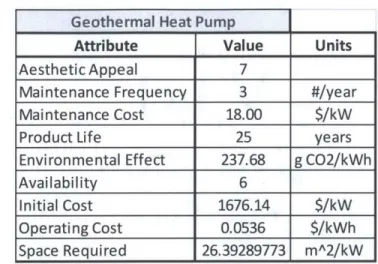
3.2.9 G eotherm al Heat Pump ... 53
3.3 Sum m ary ... 55
Chapter 4 Modification of Epoch-Era Analysis for Application to DG System Selection ... 59
4.1 Introduction ... 59
4.2 M ethodology ... 59
4.2.1 Process 1: V alue-D riving Context Definition ... 61
4.2.2 Process 2: V alue-Driven Design Form ulation... 62
4.2.3 Process 3: Epoch Characterization ... 64
4.2.4 Process 4: D esign-Epoch Tradespace Evaluation ... 66
4.2.5 Process 5: Single Epoch Analyses... 71
4.2.7 Process 7: Era Construction... 74
4.2.8 Process 8: Single-Era A nalyses ... 74
4.2.9 Process 9: M ulti-Era A nalysis ... 75
4.3 Sum m ary ... 76
Chapter 5 D istributed G eneration Case Study ... 77
5.1 Introduction ... 77
5.2 A dapted EEA for D G ... 77
5.2.1 Process 1: V alue-D riving Context D efinition ... 78
5.2.2 Process 2: V alue-D riven D esign Form ulation... 80
5.2.3 Process 3: Epoch Characterization ... 81
5.2.4 Process 4: D esign-Epoch Tradespace Evaluation ... 86
5.2.5 Process 5: Single Epoch Analyses... 95
5.2.6 Process 6: M ulti-Epoch A nalysis ... 101
5.2.7 Process 7: Era Construction... 103
5.2.8 Process 8: Single-Era A nalyses ... 105
5.3 Sum m ary ... 113
Chapter 6 H om eow ner D ifferentiation ... 115
6.1 H om eow ner 4 ... 115
6.2 H om eow ner 2... 129
6.3 Sum m ary ... 142
Chapter 7 Conclusions, A dditional Thoughts, and Future W ork... 145
7.1 Conclusions ... 145
7.1.1 EEA Form ulation for D G Selection ... 146
7.1.2 Benefit of Individual H om eow ner A nalysis ... 147
7.2 A dditional Thoughts... 148
7.3 Future W ork ... 150
Appendix A : Survey Instrum ent ... 153
A ppendix B : Epoch Tradespaces for H om eow ner 4 and 2... 155
A ppendix C : H om eow ner Survey Results ... 159
LIST OF FIGURES
Figure 1-1: Transition from Central to Distributed Generation (Farrell, 2011) ... 17
Figure 2-1: A typical microgrid structure including loads and DER units serviced by a distribution system (K atiraei, et al., 2008)... 26
Figure 2-2: A representation of the fuzzy Pareto metric, where K is the level of "fuzziness" applied to the traditional Pareto front (Schaffner, et al., 2014). ... 31
Figure 2-3: Types of trades: 1) local points, 2) frontier points, 3) frontier sets, 4) full tradespace exploration. (R oss & H astings, 2005)... 33
Figure 2-4: System Needs versus Expectations across Epochs of the System Era (Ross & R h o d es, 2 0 0 8 ). ... 3 5 Figure 3-1: Solar photovoltaic performance across all attributes. ... 41
Figure 3-2: Solar hot water performance across all attributes. ... 43
Figure 3-3: Wind turbine performance across all attributes. ... 44
Figure 3-4: Heat pump performance across all attributes... 46
Figure 3-5: Natural gas generator performance across all attributes. ... 48
Figure 3-6: Diesel generator perfonnance across all attributes. ... 49
Figure 3-7: Propane generator performance across all attributes. ... 51
Figure 3-8: Heating oil performance across all attributes... 53
Figure 3-9: Geothermal heat pump performance across all attributes... 54
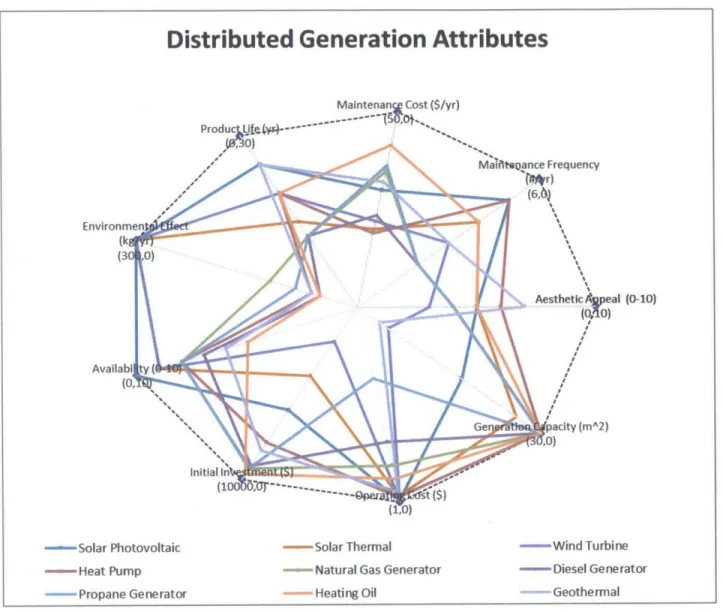
Figure 3-10: Comparison of all the distributed generation system performance attributes with the m axim um score on the perim eter... 56
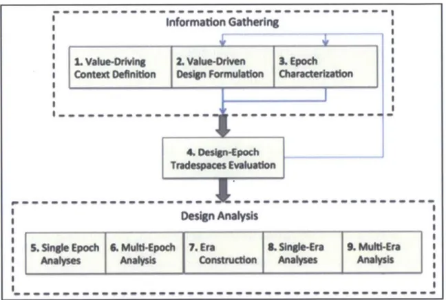
Figure 4-1: A Graphical Overview of the Gather-Evaluate-Analyze Structure of the Method (Schaffner, W u, Ross, & Rhodes, 2013)... 60
Figure 4-2: Stakeholder System D iagram ... 61
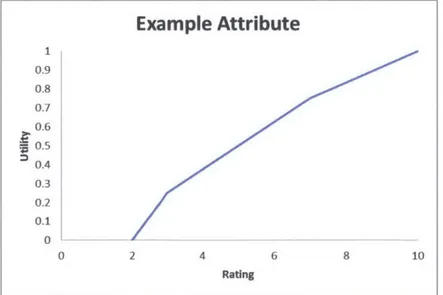
Figure 4-3: Single Attribute Expense (SAE) curve based on an example system attribute. ... 68
Figure 4-4: Single Attribute Utility (SAU) curve based on an example system attribute... 68
Figure 4-5: Examples of evaluated designs for different epochs. (Schaffner, Ross, & Rhodes, 2 0 14 ) ... 7 2 Figure 4-6: Example epoch selection for a single era. (Schaffner, Ross, & Rhodes, 2014)... 75
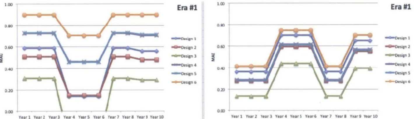
Figure 4-7: Example MAU and MAE values for each design in an era. (Schaffner, Ross, & R h o d es, 2 0 14 ) ... 7 5 Figure 5-1: A Graphical Overview of the Gather-Evaluate-Analyze Structure without including p ro c e ss 9 ... 7 8 Figure 5-2: Complex system diagram of the homeowner distributed generation network. ... 79
Figure 5-3: Simplified system diagram of the homeowner distributed generation network. ... 79
Figure 5-4: The exogenous factors that cross the system boundary and interact with the primary stak eh o ld er sy stem ... 82
Figure 5-5: Single attribute expense curves based on Table 5-6. ... 87
Figure 5-6: Single attribute utility curves based on Table 5-8... 91
Figure 5-7: Visual tradespace (MAE v. MAU) for the baseline epoch. ... 95
Figure 5-8: The evaluated designs for each of the 10 non-baseline epoch periods... 100
Figure 5-9: Normalized Pareto Trace of the design choices over all 11 epochs... 101
Figure 5-10: Trend of NPT for design choices after inclusion of "fuzzy" boundary. ... 103
Figure 5-11: Design choice values across each of the epoch in Eral (Environment) moving from left to right and top to bottom . ... 106
Figure 5-12: Environmental era MAE and MAU values for each design choice over 12 years. 107 Figure 5-13: Implementation of the operational value metric across the environmental era for all D G sy stem s. ... 10 8 Figure 5-14: Design choice values across each of the epoch in Era2 (Cost) moving from left to right and top to bottom in per English language reading rules... 109 Figure 5-15: Cost era MAE and MAU values for each design choice over 12 years... 109 Figure 5-16: Implementation of the operational value metric across the cost era for all DG
sy stem s... 1 10 Figure 5-17: Design choice values across each of the epoch in Era3 (Hi-Tech) moving from left to right and top to bottom in per English language reading rules... 111 Figure 5-18: Hi-Tech era MAE and MAU values for each design choice over 12 years... 112 Figure 5-19: Implementation of the operational value metric across the hi-tech era for all DG sy stem s... 1 13 Figure 6-1: Comparison between average homeowner and Homeowner 4 preferences when selecting distributed generation system s... 116 Figure 6-2: The difference in the baseline tradespace between the average homeowner (blue) and Homeowner 4 (red). The Pareto Frontier is represented by the appropriate dotted line. ... 117 Figure 6-3: The difference in the product available tradespace between the average homeowner (blue) and Homeowner 4 (red). The Pareto Frontier is represented by the appropriate dotted line.
... 1 1 8 Figure 6-4: Trend of NPT for design choices after inclusion of "fuzzy" boundary for the average homeowner (blue) and Homeowner 4 (red). The results from Homeowner 4 are layered onto the average hom eow ner results... 119 Figure 6-5: Environmental era MAE and MAU values for each design choice over 12 years for the average hom eow ner. ... 120 Figure 6-6: Environmental era MAE and MAU values for each design choice over 12 years for H om eow n er 4 ... 12 1 Figure 6-7: Comparison of the operational value metric across the environmental era for the average homeowner (blue) and Homeowner 4 (red). ... 121 Figure 6-8: Cost era MAE and MAU values for each design choice over 12 years for the average h o m eo w n er... 12 3 Figure 6-9: Cost era MAE and MAU values for each design choice over 12 years for
H om eow n er 4 ... 12 3 Figure 6-10: Comparison of the operational value metric across the cost era for the average hom eowner (blue) and H om eowner 4 (red)... 124 Figure 6-11: Hi-Tech era MAE and MAU values for each design choice over 12 years for the average hom eow ner. ... 126 Figure 6-12: Hi-Tech era MAE and MAU values for each design choice over 12 years for
H om eow n er 4 ... 12 6 Figure 6-13: Comparison of the operational value metric across the hi-tech era for the average hom eowner (blue) and H om eow ner 4 (red)... 127 Figure 6-14: Comparison between average homeowner and Homeowner 2 preferences when selecting distributed generation system s... 129 Figure 6-15: The difference in the 50% cost of maintenance tradespace between the average homeowner (blue) and Homeowner 2 (red). The Pareto Frontier is represented by the appropriate d o tted lin e ... 13 0
Figure 6-16: The difference in the neighbor agreeing tradespace between the average homeowner (blue) and Homeowner 2 (red). The Pareto Frontier is represented by the appropriate dotted line. ... 1 3 1 Figure 6-17: Trend of NPT for design choices after inclusion of "fuzzy" boundary for the average
hom eow ner (blue) and H om eowner 2 (red)... 132
Figure 6-18: Environmental era MAE and MAU values for each design choice over 12 years for the average hom eow ner. ... 134
Figure 6-19: Environmental era MAE and MAU values for each design choice over 12 years for H o m eo w n er 2 ... 134
Figure 6-20: Comparison of the operational value metric across the environmental era for the average homeowner (blue) and Homeowner 2 (red). ... 135
Figure 6-21: Cost era MAE and MAU values for each design choice over 12 years for the average h om eow n er. ... 136
Figure 6-22: Cost era MAE and MAU values for each design choice over 12 years for H o m eo w n er 2 ... 13 6 Figure 6-23: Comparison of the operational value metric across the cost era for the average hom eow ner (blue) and H om eow ner 2 (red)... 137
Figure 6-24: Hi-Tech era MAE and MAU values for each design choice over 12 years for the averag e h om eow n er. ... 139
Figure 6-25: Hi-Tech era MAE and MAU values for each design choice over 12 years for H o m eo w n er 2 ... 13 9 Figure 6-26: Comparison of the operational value metric across the hi-tech era for the average hom eow ner (blue) and H om eowner 2 (red)... 140
Figure 6-27: All interviewed homeowner preferences when selecting distributed generation system s com pared to the average "hom eowner". ... 142
Figure B-1: The evaluated designs for each of the 11 epoch periods for Homeowner 4. ... 156
Figure B-2: The evaluated design for each of the 11 epoch periods for Homeowner 2... 158
LIST OF TABLES
Table 3-1: Key description of the example homeowner's energy use and desired DG portfolio. 37
Table 3-2: Solar photovoltaic (PV) values considered for this case study. ... 41
Table 3-3: Solar hot water values considered for this case study... 42
Table 3-4: Wind turbine values considered for this case study. ... 44
Table 3-5: Heat pump values considered for this case study... 45
Table 3-6: Natural gas generator values considered for this case study... 47
Table 3-7: Diesel generator values considered for this case study. ... 49
Table 3-8: Propane generator values considered for this case study. ... 50
Table 3-9: Heating oil furnace values considered for this case study... 52
Table 3-10: Geothermal heat pump values considered for this case study... 54
Table 3-11: Summary of all nine DG systems and their performance across all nine attributes.. 55
Table 4-1: Prim ary Stakeholder A ttributes... 62
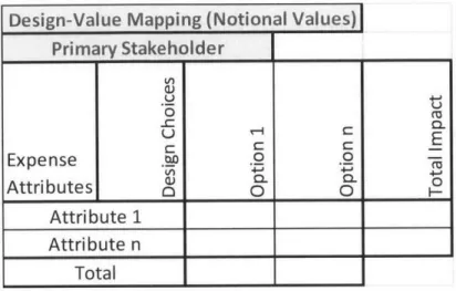
Table 4-2: A Design-Value Matrix reflecting the notional impact of design variables on expense attrib u te s... 6 3 Table 4-3: A Design-Value Matrix reflecting the notional impact of design variables on utility attrib u te s... 6 3 Table 4-4: Epoch D escriptions... 64
Table 4-5: A matrix reflecting the notional impact of epoch variables on expense attributes. .... 65
Table 4-6: A matrix reflecting the notional impact of epoch variables on utility attributes... 65
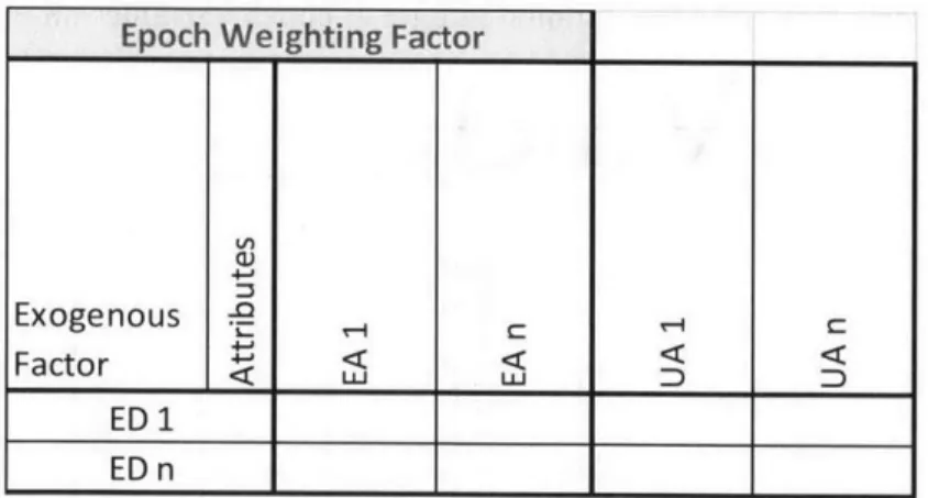
Table 4-7: The epoch weighting factors for both expense and utility attributes. ... 66
Table 4-8: Single Attribute Expense (SAE) values for the system expense attributes... 67
Table 4-9: Single Attribute Utility (SAU) values for the system utilty attributes... 67
Table 4-10: The evaluated attributes for each design choice with MAE and MAU values. ... 70
Table 4-11: The MAE values of the design choices for the epoch descriptors. ... 71
Table 4-12: The MAU values of the design choices for the epoch descriptors... 71
Table 4-13: The NPT for each design across all epochs... 73
Table 4-14: NPT and fNPT of the design choices. ... 73
Table 4-15: Construction of Eras including the epoch sequencing and duration. ... 74
Table 5-1: California hom eowner attributes. ... 80
Table 5-2: Characterization of epochs that represent exogenous factors from Figure 5-4... 82
Table 5-3: A matrix reflecting the notional impact of the epoch variables on the expense attrib u te s... 8 4 Table 5-4: A matrix reflecting the notional impact of the epoch variables on the utility attributes. ... 8 5 Table 5-5: The weighting factors of the epochs for both the expense and utility attributes... 85
Table 5-6: Single attribute expense values for distributed generation systems... 87
Table 5-7: MAE k factors for each epoch determined from the homeowner interviews. ... 88
Table 5-8: Single attribute utility values for distributed generation systems. ... 90
Table 5-9: MAU k factors for each epoch determined from the homeowner interviews... 92
Table 5-10: The evaluated attributes for each design choice with MAE and MAU values. ... 93
Table 5-11: The evaluated M AE values for all epochs... 96
Table 5-12: The evaluated M AU values for all epochs. ... 97 Table 5-13: Joint MAE and MAU feasibility of the distributed generation systems over all
Table 5-14: The NPT for each design across all 11 epochs... 101 Table 5-15: NPT and fNPT of the distributed generation design choices over all 11 epochs.... 102 Table 5-16: Era construction of likely scenarios from the represented epochs... 104 Table 5-17: Summary of the average homeowner distributed generation system selection through each analysis with Ist in green, 2 in yellow, and 3rd in orange... 114 Table 6-1: Difference in the fNPT values between Homeowner 4 and the "average" homeowner. ... 1 2 0 Table 6-2: Difference in the operational value metric between Homeowner 4 and the "average" hom eow ner for the environm ental era. ... 122 Table 6-3: Difference in the operational value metric between Homeowner 4 and the "average" hom eow ner for the cost era... 125 Table 6-4: Difference in the operational value metric between Homeowner 4 and the "average" hom eow ner for the hi-tech era. ... 127 Table 6-5: Summary of Homeowner 4 distributed generation system selection through each analysis with 1st in green, 2 nd in yellow, and 3 rd in orange. ... 128
Table 6-6: Difference in the fNPT values between Homeowner 2 and the "average" homeowner. ... 1 3 3 Table 6-7: Difference in the operational value metric between Homeowner 2 and the "average" hom eow ner for the environm ental era. ... 135 Table 6-8: Difference in the operational value metric between Homeowner 2 and the "average" hom eow ner for the cost era... 138 Table 6-9: Difference in the operational value metric between Homeowner 2 and the "average" hom eow ner for the hi-tech era... 140 Table 6-10: Summary of Homeowner 2 distributed generation system selection through each analysis with 1st in green, 2 in yellow, and 3rd in orange. ... 141 Table 6-11: Summary of the top three selections for the average homeowner, Homeowner 2, and Homeowner 4 across the different analyses with 1st in green, 2 in yellow, and 3rd in orange. 143
LIST OF ABBREVIATIONS
CO2 Carbon Dioxide
DG Distributed Generation
EEA Epoch-Era Analysis
fNPT Fuzzy Normalized Pareto Trace
GHG Greenhouse Gas
kW Kilowatt
LCOE Levelized Cost of Electricity
MAE Multi-attribute expense
MAU Multi-attribute utility
NPT Normalized Pareto Trace
SAE Single attribute expense
SAU Single-attribute utility
SEAri System Engineering Advancement Research Institute
Chapter 1 Introduction 1.1 Background and Motivation
Power generation in the United States has largely remained stagnant for a large part of the previous century with the centralized power distribution network. This style of distributed network structure resulted in centralized generation facilities that were connected to consumers with massive transmission and distribution networks. Centralized power structures did not provide the consumer with the ability to generate their own power through renewable and non-traditional generation methods. The Intergovernmental Panel on Climate Change's (IPCC) report indicating the existence of global warming (IPCC Third Assessment Report, 2001) created a shift in public desire to attain energy from renewable resources. When this sentiment shift was
coupled with legislation that was restructuring and deregulating the power sector and increasing technological power innovation, a new power generation model became possible - distributed generation.
Centralized
Power
C
DtJrutian noiwork
Figure 1-1: Transition from Central to
lean, local power
4(
Distributed Generation (Farr
HP I
ell, 2011)
Over the past ten years distributed generation (DG) has started to become economically viable for the average homeowner to install and utilize for their energy needs, due in large part to increased focus placed on finding a solution to curb the increasing global warming trend. As such, there are a number of DG technologies that the homeowner can select, each having their own advantages and disadvantages in certain possible scenarios over the life of the system. This leads to a large degree of uncertainty for the homeowner when trying to determine which DG technologies are most attractive for meeting their needs or even their risk profile, a potentially
formidable challenge. Therefore, the homeowner would benefit from a structured approach for comparing the different DG systems across various scenarios, assisting them in determining their most appropriate DG system. This thesis provides an example application of a structured system
engineering method for DG system decision. Additionally, two individual homeowner cases are analyzed to determine whether an average of homeowner information can be used or if
individual analysis must be performed on each homeowner.
Additional motivation for pursuing this research is from a provider perspective, complementing the homeowner perspective decision problem above. The author has recently started a solar thermal company and is trying to determine the value that the distributed generation system will provide to homeowners in southern California. Since there has not been a widely accepted or publicized method for comparing distributed generation systems, it is difficult to determine where there are unmet homeowner needs. By performing the analysis for all DG systems
available to the homeowner, the author will be able to gather insight into where these gaps in the tradespace are and how a new system might be able to provide value to the homeowner.
1.2 Research Scope
Based on the background and motivation aforementioned, the primary focus of the thesis is to create a multi-attributed expense (MAE) and multi-attribute utility (MAU) function - detailed in section 2.2 - that enables the comparison of distributed generation systems using multiple decision making criteria. The variables for the MAU and MAE function will be determined by
investigating the preferences of homeowners in Southern California - gathered by in-person interviews - along with collecting data provided by the Department of Energy and other
validated resources. These functions will formalize, structure, and make explicit the homeowner preferences on costs and benefits of potential DG systems. This approach enables the researcher to generate homeowner scores for each alternative system and compare them on a common basis.
Since preferences for the homeowner, as well as the performance of DG systems may be
impacted by exogenous factors - also referred to as scenarios in this thesis - another component of the research is to evaluate how the score changes for each DG system based on a number of exogenous factors that may occur during the product's lifetime. These changes in the utility value score will provide an indication into which of the DG systems are more robust for each of the given scenarios. A third component of the research will be to evaluate the distributed
generation systems across a sequence of the exogenous factors which will represent how the utility value of each system might change over time. By evaluating the change in utility value over time, the homeowner will have a better understanding of which DG system will provide the greatest benefit over the product's life. This approach forms the basis of the Epoch-Era Analysis (EEA) method - described in greater detail during section 2.4 - which provides for visualization
and a structured way to think about the temporal system value environment (Ross & Rhodes, 2008).
The final component will be to select a couple of homeowners with vastly different preferences and analyze the best DG system for them based on the previous steps. The results of the analysis will be used to demonstrate that the selection of the average homeowner case may not be the most attractive choice for each homeowner. Therefore, it is more beneficial to find better solutions for each of the individual stakeholders instead of providing a singular solution to all homeowners. To summarize the research, the benefits and limitations will be discussed along with proposed recommendations for future research work.
1.3 Research Objectives
The main objective of the research is to evaluate the different technologies for distributed generation that the Southern California homeowner has available to them and provide the homeowner with a score that can be used to compare the DG systems. The research will
incorporate exogenous factors into the resulting scores for each distributed generation system to account for externalities that affect the homeowner's decision making process, but are out of their control. A secondary objective of the research is to provide homeowners with a possible
scenario of exogenous factors over the life of the system and capture the utility value created by the system over time. The final objective of the research is to provide evidence - through a few
example homeowner cases - whether the "average homeowner" selection matches their
individual selection. In summation, these objectives can be described by the following research questions:
* Given an Epoch-Era Analysis formulation, which of the distributed generation power system choices available to the southern California homeowner provides the highest
value across the greatest number of epochs and in a select number of potential era scenarios?
* Using the same Epoch-Era Analysis formulation, how does the highest value distributed generation choice for randomly selected homeowners differ from that of the highest value for the homeowner subset average?
1.4 Organization of Thesis
Chapter 2 provides a literature review of distributed generation, methods for tradespace analysis, Multi-Attribute Utility Theory, and Pareto efficiency. Broader discussions will cover the
definition of distributed generation and how it is starting to become available to homeowners. This will be followed by a discussion of tradespace analysis methods utilized by the MIT
Systems Engineering Advancement Research Initiative (SEAri). Focus will be placed on the methodologies' structure and how they have been previously applied, along with stating how they can be utilized in other technical areas. The author will then proceed to introduce Multi-Attribute Utility Theory, which is a key component of evaluating how differing choices can be
compared and analyzed. Lastly, Pareto efficiency - another core concept in the methods - will be explained as it pertains to tradespace analysis and the more specific instruments that are utilized in this thesis.
Chapter 3 will introduce the representative homeowner considered in the study and his available distributed generation system choices. The demographic information that was used to select the homeowners' decision making criteria used for the research will be presented. Following this will be an explanation of the distributed generation systems available to the homeowner and their
associated performance metrics of interest to the homeowner, derived from system brochures and government data sources.
Chapter 4 provides the framework that is used in Epoch-Era Analysis when applied to system selection, as opposed to the more traditional system design application. The chapter begins by describing the overarching framework and then decomposes the framework into actionable steps that can be used for the analysis. Each of the steps or processes will include the information that needs to be gathered and produced for providing the desired end result. The author will indicate the modifications to the overarching method for the chosen application and also indicate which of the processes will not be employed.
Chapter 5 utilizes each step in the methodology proposed in Chapter 4 for the average homeowner DG system selection case example. This includes describing the modification to Epoch-Era Analysis methodology and detailing the abstracted system used in the analysis. The steps used to create the model that generates the tradespace analysis and how the utility functions were created to determine the scores for each DG system will be presented. Following the model creation step will be the analysis and results of the epoch periods. Comparison of the epochs to one another will also be displayed in the chapter alongside preliminary determination of trends for each DG system. The author will propose a select number of era scenarios based on research from sources about the likely trend of events over the next period of time - although it will not be an all-inclusive list of possible scenarios.
Chapter 6 evaluates the effect of the individual homeowner attributes on the resulting "best" distributed generation system selection for the aggregate homeowner in Chapter 5. This is done by comparing the best distributed generation resource for the average homeowner to the best DG resource for a couple of randomly selected homeowners. These randomly selected cases will be presented to demonstrate how the average homeowner selection did not match the selection for
the individual homeowners and in this case, the interview participants.
Chapter 7 summarizes the answers to the research questions provided by the thesis and indicates areas where future work could strengthen the presented results.
1.5 Data of Thesis
The thesis data for the background information is derived from a literature review of publically available information, while the detailed technical information on the DG systems is summarized from product brochures, interviews with industry experts and government websites. There are a multitude of DG systems available to the homeowner and the systems presented are understood to not be an all-inclusive representation. Information about homeowner preferences is attained from one-on-one interviews with homeowners and their results were anonymized to meet MIT Committee on the Use of Humans as Experimental Subjects (COUHES) standards. Similar to the DG system performance metrics, the number of interviews and information gathered is not intended to represent the entire population of southern California but is intended to be a representative subset. The model and method is still applicable to a larger sample size and tlie
appropriateness of this application is discussed later in the thesis. Some of the data has been inferred by the author, since there are a number of different estimates of possible scenarios of exogenous factors and these inferences are only used to provide examples of how the method
could be used to provide results when the data becomes available. Lastly, any of the data presented in this thesis should be independently verified as there are a number of factors that change across the population and over different periods of time as world events continue to shape our responses to different scenarios.
Chapter 2 Literature Review 2.1 Distributed Generation
As mentioned previously in section 1.1, the large majority of residences in the United States receive their power from traditional power systems. These traditional power systems are large
generation plants that are geographically isolated from the population where the power is transferred via long distance transmission lines to the end consumer. This type of system requires monitors and system control centers to ensure that the power delivered to the end user meets the required standards (Blaabjerg, et al., 2004).
While the traditional power systems have been successful for a number of years, sentiment has begun to shift about the use of fossil fuels to generate power for the majority of the worldwide economy. Additionally, the traditional power systems are struggling to keep up with the daily increase in demand for energy and the challenges of maintaining the required power standards are manifesting in the form of outages. These two primary factors have driven interest in clean technology development that could be placed closer to the population centers in larger quantities but smaller capacities (Blaabjerg, et al., 2006).
The term for this new concept for power generation systems started out being called dispersed
generation, but has more recently been called distributed generation or simply abbreviated as
DG. Since DG power systems are much smaller than traditional power systems, they can be
placed closer to or within population centers to take advantage of previously untapped renewable and nonconventional energy sources. This ability to generate additional power near the end user
has been welcomed into the energy management systems in most countries and has become part of their long term energy solution plans (Guerrero, et al., 2010).
DG systems come in a variety of different forms and technologies to capture previously untapped renewable resources, which include, but are not limited to, solar photovoltaic cells, wind
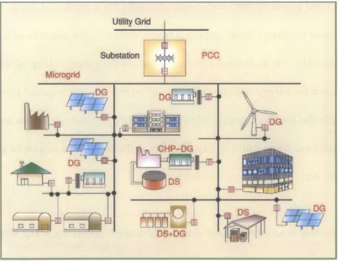
turbines, fuel cells, and combined heat and power turbine (Blaabjerg, et al., 2004). These new technologies have enabled new formations of distribution grids to take place, as seen in Figure
2-1, which capitalize on the different characteristics of the technologies to provide a more efficient and effective power delivery system (Katiraei, et al., 2008).
Utility Grid Substation PCC Microgrid DGG CHP-DG rnGD DS+DG
Figure 2-1: A typical microgrid structure including loads and DER units serviced by a distribution system (Katiraei, et al., 2008).
Microgrid is the term typically used for the new formation of the distribution grid that enables
the integration of DG technologies due to its ability to be a self-contained grid on a significantly smaller scale than the traditional power grid structure. The arrangement in Figure 2-1 is
connected to the traditional power grid, but as described above, it is expected to operate as a standalone entity. This arrangement style enables the DG technologies to work in tandem to deliver reliable power according to the required power standard, something that renewable technologies have had a difficult time meeting in the traditional power systems scale (Katiraei, Iravani, Hatziargyriou, & Dimeas, 2008). As a function of the ability to group renewable
resources together in the microgrid model, a number of countries are predicting that there will be much higher percentages of power that will be delivered from a DG resource (Blaabjerg, et al., 2004).
The rise of microgrids and distributed generation as possible solutions to the problems currently experienced by the larger grid creates a new problem about determining which solutions should be incorporated. This problem needs to be addressed beyond selecting the most popular
technology at the time and multi-criteria decision making techniques could provide useful in this regard.
2.2 Multi-Attribute Utility Theory (MAUT)
Utility theory was first introduced in 1947 by Von Neumann and Morgenstern (Von Neumann & Morgenstern, 1947) and in its most basic form maps the outcome of an action to a subjective measure of value. According to the theory in the above terms, a rational individual will act in a manner that would maximize their value. In order to generate mathematical equations which could characterize these choices, the authors denoted the action as an attribute and the value as the associated utility. Also, four axioms were generated to characterize rationality through three hypothetical lottery outcomes H, J, and K:
1. For two lotteries H and J, either H is preferred to J, J is preferred to H, or the individual is indifferent between H and J (completeness axiom).
2. If H is preferred to J and J is preferred to K, then H is preferred to K (transitivity axiom). 3. If H is preferred to J and J is preferred to K, then a probability p exists such that an
individual is indifferent between pH + (1 -p)K and J (continuity axiom).
4. For the three lotteries, H is preferred to J if and only if pH + (1-p)K is preferred to pJ + (l-p)K (independence axiom). (Von Neumann & Morgenstern, 1947)
Based on the work of Von Neumann and Morgenstern, Keeney and Raiffa expanded utility theory to cover instances where there were multiple attributes that concurrently contributed to value. This work became the foundation of Multi-Attribute Utility Theory (MAUT). MAUT enables the classification of user decisions with regards to multiple features of a product or system at the same time, which more closely models the decision making process (Keeney & Raiffa, 1976). Instead of simply having individual scores for each of the product or system attributes - as derived in utility theory - MAUT combines the multiple single attribute utility values across the desired attributes into a single multi-attribute utility value. The single value can then be used to compare multiple products or systems to one another to determine which creates the greatest combined utility for the stakeholder. MAUT can be expressed as the following mathematical equation:
U(X) = u(x, k)
Equation 2-1: Multi-attribute utility function.
Equation 2-1 can be represented in a number of ways and the simplest is the linear-additive form shown in Equation 2-2 where the desire to represent the decision maker's preferences accurately
is balanced by the need to maintain simplicity. Additionally, to utilize this form of the equation the features of the system need to maintain an independent relationship with how they affect the overall utility (Keeney & Raiffa, 1976). For the case that will be presented throughout this body of work, Equation 2-2 will be used to calculate the multi-attribute utility of the proposed DG designs. Shown here is the mathematical representation:
n
U(X) = 1k -u(xi)
i=1
Equation 2-2: Linear-additive form of the multi-attribute utility function.
where n values of k - acting as a weighting mechanism - sum to one and u - representing the
single attribute utility value for attribute xi- ranges from zero (worst) to one (best), resulting in the multi-attribute utility value U, ranging from zero (worst) to one (best), for the vector X of all attributes.
MAUT is clearly a power approach that creates a single value for multi-criteria decision making situations, but this new information generates a problem when trying to determine how to select a system based on the their respective values. Pareto Optimality is one solution to the problem that could provide useful in selecting the appropriate DG system based upon multi-attribute values.
2.3 Pareto Optimality
Sometimes evaluated design alternatives are compared to one another across more than one factor, such as MAU - the utility metric of the system - and the cost metric of the system. Conceptually this comparison can be considered as the affordability tradeoff (what do you get benefit-wise, for different expenditure of cost?). This comparison across multiple factors without
aggregation into a single metric is called a tradespace and different analysis tools for tradespaces will be described in section 2.4. ("Tradespace" is an amalgamation of "trades" and "space" representing that there is a space of tradeoffs where no "best" solution exists without further determining how to evaluate the tradeoffs. This formulation promotes knowledge generation, especially for complex systems where the relationship between costs and benefits may not be obvious a priori.) In the tradespace, multiple designs are compared against each other and a common approach that is used to determine the better designs is the concept of Pareto
Optimality, often used in multi-objective analysis. In other words, "Pareto Optimality is achieved when a solution is non-dominated, that is, a solution cannot be improved in a particular objective score without making other objective scores worse" (Ross, et al., 2009).
2.3.1 Pareto Frontier
In most tradespaces there is not a single design that is considered the ultimate best as the
intention is to provide insight to a decision maker for understanding the result of a design choice (the cost versus benefit tradeoff that may not be well understood in advance). Still, there are designs that can be considered better than the other designs given a certain set of decisions or attributes. For example, there could be a design solution that has the highest utility while having the greatest cost or having the least cost while having the lowest utility.
As described in Ross, Rhodes, and Hastings, the concept of Pareto Optimality can be applied to the tradespaces created by MAUT which results in a number of non-dominated solutions in the tradespace (Ross, et al., 2009). These design solutions result in a boundary in which there are no designs that perform better than the boundary design for that given set of objective metrics. The designs on the frontier represent the most efficient tradeoff of cost and benefit (e.g. MAU) and
reduce the tradespace under consideration, providing a simpler subset for comparison by the decision maker.
2.3.2 Fuzzy Pareto Number
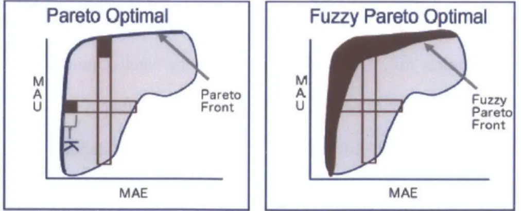
Although careful analysis is used when creating the values that generate tradespaces, there are instances where uncertainty may exist - especially in cases where the design is highly conceptual or the data tends to vary on uncontrollable factors. One method that can be used to address the uncertainty is to incorporate "fuzziness" into the Pareto Frontier. The fuzzy factor is represented by a fraction or percentage of the Pareto Optimal values, which results in a range of values that are considered part of the non-dominated space (Smaling, 2005). By increasing the acceptable range of values that are non-dominated, the number of designs that a decision maker chooses from may increase to include designs with uncertainty that were near the Pareto Optimal (Ross, et al., 2009). Summarizing the concepts from section 2.3. land this section, Figure 2-2 presents images that clarify the concept of the Pareto Optimal solution and the effect of including a fuzzy factor to that solution.
Pareto Optimal
M
A Pareto
U Front
MAE
Fuzzy Pareto Optimal
M
A Fuzzy
U Pareto
Front
MAE
Figure 2-2: A representation of the fuzzy Pareto metric, where K is the level of "fuzziness" applied to the traditional Pareto front (Schaffner, et al., 2014).
2.3.3 Normalized Pareto Traces
A method that can be employed by product or system designers is to create multiple tradespaces through the consideration of systems in different short run scenarios, or epochs, to determine how a particular system performs under different circumstances. When multi-tradespace analysis is coupled with standard Pareto Optimality for each design, then the result is called a Pareto Trace. According to Ross, Rhodes, and Hastings, a Pareto Trace is defined as "the number of Pareto Sets containing that design," (Ross, et al., 2009).
To achieve a Normalized Pareto Trace (NPT), the Pareto Trace must be divided by the total number of Pareto Sets analyzed, which then results in a fractional representation of the number of occurrences where the design is part of the Pareto Set. Normalized Pareto Trace is often used as a metric to determine which of the designs are most passively value robust for the given scenarios investigated (these designs stay utility-cost efficient across a large fraction of considered scenarios) (Ross, et al., 2009).
2.3.4 Fuzzy NPT
Similar to how uncertainty may need to be addressed for the Pareto Optimality, there may be the desire to determine the amount of uncertainty in the Normalized Pareto Trace for each design. According to Ross, Rhodes, and Hastings the Fuzzy Pareto Trace is defined as "the number of Fuzzy Pareto Sets containing that design" (Ross, et al., 2009). Typically the amount of fuzziness - represented by the factor K - is varied to determine how often the design is part of the Pareto Set, which defines the band of new Pareto values. To achieve the Fuzzy NPT value, the Fuzzy Pareto Trace number is dived by the number of total number of Pareto Sets analyzed. Fuzzy NPT
is another metric that can be used to determine the passive value robustness of a design with uncertain characteristics and over a number of potential scenarios.
2.4 Select System Engineering Methods for Tradespace Analysis
Tradespaces are can be helpful tools when selecting between different design and characterizing the advantages and disadvantages given certain scenarios or desired performance metrics. Research has been performed at MIT to determine how tradespaces can be better utilized by decision makers - where better can be exemplified through either simpler implementation, a more complete representation of the factors involved (Ross, 2006). Ross and Hastings (2005) identified that there were four types of trades that are most common, which are represented in Figure 2-3. Value 32 41 0 0 0 ee .. :0 Cost
Figure 2-3: Types of trades: 1) local points, 2) frontier points, 3) frontier sets, 4) full tradespace exploration. (Ross & Hastings, 2005)
As one steps through the different types of trades in increasing order, the level of effort that is required to develop a relevant solution also increases - moving from a local point solution to
frontier subset to frontier solution set to full tradespace exploration - but the higher effort trades also provide the greatest level of detail, allowing for greater insights into the appropriate design
(Ross & Hastings, 2005). In this research, the full tradespace will be explored with the majority of the analysis focused on the frontier solutions.
Beyond identifying the types of trades that are available for selecting the appropriate design, a number of methodologies can be used to properly set up a tradespace analysis to ensure positive results. In his work from 2006, Ross describes an end-to-end process called Multi-Attribute Tradespace Exploration (MATE) to develop and explore the tradespace that covers the problem
identification to generating a utility value. The steps of the process are to: 1. Identify decision-maker needs by eliciting attributes and preferences. 2. Generate attribute utility functions through formal stakeholder interviews. 3. Aggregate utilities into multi-attribute utility function.
4. Propose design solutions to perform well in attributes.
5. Develop models to link solutions to decision-maker value.
6. Apply multi-attribute utility function to evaluated design solutions. 7. Plot utility and other important metric - often a form of cost.
8. Explore the tradespace to generate knowledge of nonobvious trade-offs.
Typically this process utilizes parametric or other numerical computer models that can evaluate a large number of designs while providing the attribute metrics and system costs that are ultimately plotted to create the fully developed tradespace (Ross, 2006).
A weakness of traditional tradespace exploration approaches is that they often assume a static contextual reference for the lifespan of the analysis. This may not be a realistic assumption when scenarios are modeled, leading to inconsistencies and inaccuracies in design selection.
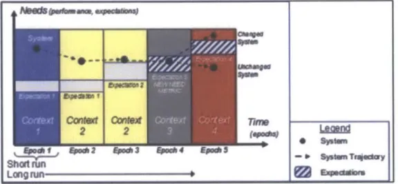
Additionally, this prevents a thorough understanding of the system value across the design's lifespan (Ross & Rhodes, 2008). Building upon the foundation of a strong tradespace analysis, an analysis method to consider the impacts of context changes during the associated timeline called Epoch-Era Analysis (EEA) was developed (Ross, 2006). Considering the impact of context changes enables a more thorough and accurate representation of the desired scenarios (Ross & Rhodes, 2008). Figure 2-4, shown below, illustrates how the context changes, impacting the success of a design, are manifested in the method.
' y~SPUTiq.cwyI
Shot run
Lonig run____ ____
Figure 2-4: System Needs versus Expectations across Epochs of the System Era (Ross & Rhodes, 2008).
An epoch is a time period of fixed contexts and needs, sometimes called a "short run scenario."
The context and needs may change over time (as represented by exogenous factors). Epochs can also be considered "state scenarios" representing one possible configuration of the exogenous
factors (Ross, et al., 2009). An era is defined as an ordered sequence of epochs and represents a potential "long run scenario." A collection of epochs form an era and that era varies depending
on the composition of the contexts incorporated since each era does not include every context considered in the analysis (Ross & Rhodes, 2008). This form of analysis enables a broad
timescale and context understanding of system performance while also using existing tradespace methods including Multi-Attribute Tradespace Exploration (Ross, et al., 2009). The Epoch-Era Analysis formulation used in this research will be addressed in greater detail throughout Chapter
4.
2.5 Summary
Each section of this literature review is meant to build upon each other to provide a base understanding before each of the topics are covered in further depth in the subsequent chapters. The foundation of the research is on distributed generation systems that are available for homeowners. Building on top of this is the need to translate the individual metrics for each system into a value that can be compared across each; therefore, an understanding of Multi-Attribute Utility Theory is needed. Since the systems offer different value for their respective costs, it is important to understand various topics surrounding Pareto Optimality through the concept of a trade-off. Creating a full tradespace analysis enables further investigation into how various contexts may shape an alternative design's value over time. These foundational concepts are necessary to comprehend the Epoch-Era Analysis of distributed generation systems for homeowners.
Chapter 3 Distributed Generation Choices for the Homeowner
Chapter 3 will provide the context for the application of EEA in Chapter 5 and Chapter 6. This chapter will provide the homeowner geographical location and energy use information as well as the homeowner decision criteria. Additionally, the performance metrics of the distributed
generation systems used in the analysis will also be provided. These pieces of information are necessary to develop the foundations of the EEA formulation being investigated in the research
questions.
3.1 Homeowner Energy Use and DG Selection Criteria
When determining the distributed generation power system choices that are available to the homeowner in this analysis, it is imperative to define the region that the homeowner is from in addition to general power characteristics. The energy use information for a typical San Jose, CA homeowner is found in Table 3-1.
Homeowner (San Jose, CA)
Description Value Units
Electricity Cost 0.20 $/kWh Yearly Energy Use 6480 kWh/yr Daily Energy Use 17.75 kWh/day
DG Percentage 50%
DG Daily Operation 2 hours
DG Capacity 4.44 kW
Table 3-1: Key description of the example homeowner's energy use and desired DG portfolio.
The location of the homeowner was selected by the author for several reasons. First, the electrical power grid in California is currently undergoing a shift from traditional power generation to distributed power generation. Next, of the states shifting towards distributed
generation systems, California provides the greatest number of choices for homeowners pursuing this path. Additionally, the homeowners in this region face higher electricity rates than the
majority of the contiguous U.S. while having one of the lowest energy uses per capita, which aligns with the economics of current distributed generation solutions. Lastly, San Jose was selected due to a priori knowledge of the city and ease of locating energy use data.
Energy use data and electricity cost data for the homeowner was gathered from the Energy Information Administration website and is based on annual average consumption for the state of California (California State Profile and Energy Estimates, 2014). Although exact usage may vary depending on the homeowner, this approximation is suitable for the analysis presented. In order to achieve a more accurate analysis, a specific homeowner's usage information should replace the more general aggregate data.
In order to determine the data for the distributed generation usage, homeowners were informally polled about the amount of energy they wished to generate from non-grid technologies and how long they wished the system to operate. Again, the numbers provided in Table 3-1 for the DG usage were based on the aggregate, but numbers for a specific homeowner could be incorporated to provide a more accurate analysis. The two previously mentioned numbers resulted in the capacity of the system that would be needed to meet those homeowners' desires.
A fundamental component needed for an Epoch Era Analysis formulation - covered in greater detail in Chapter 4 and Chapter 5 - is the preferences of the primary stakeholder, which in this case is the San Jose homeowner. Using the verbal survey instrument from Appendix A: Survey Instrument, six homeowners were interviewed to determine the criteria that they would use if they were to make a distributed generation purchase. This resulted in the following nine
attributes, their definitions that these particular homeowners use during their evaluation process, and the value scales from the least preferred to the most preferred:
" Aesthetic appeal - the system's appearance when considered part of their property having a scale from zero to ten
" Maintenance frequency - the number of maintenance and service events per year that the system requires the homeowner or third party to replace, change, or fix systems or components having a scale from twelve to zero
* Maintenance cost - the total cost in dollars per year required to keep the system operating at full efficiency including parts and labor hours invcstcd by the homeowner or
designated third party having a scale from $1000 to $0
* Product life - the minimum numbers of years that the manufacturing or retailing
companies specifies that the system is able to operate before replacement having a scale from zero to fifty
* Environmental effect - the pounds of carbon dioxide (lbs. C0 2) that are produced by the
system during annual operation having a scale of 2000 to 0
* Availability - how easy is the system to acquire, by the homeowner, as a function of the number of outlets retailing the system for a given region having a scale from zero to ten * Initial cost - the total cost that the homeowner must pay to acquire the system' having a
scale from $100,000 to $0
The initial cost will be considered a one-time payment to acquire the system for this research project, but there are other methods that are also considered as the initial cost of the system - financing options, renting, power purchase agreements, etc. -that are not incorporated into this analysis.
" Operating cost - the cost that the homeowner must pay to operate the system with
specific focus on fuel or electric usage that is required to produce the homeowners desired amount of energy having a scale from $1000 to $0
" Space required - the number of square meters that are required per kilowatt of generation capacity of the system having a scale from twenty-five to zero.
3.2 DG System Alternative
With the fundamental understanding of the homeowner attributes used when evaluating a distributed generation power system, the alternatives available to the homeowner can now be discussed. The majority of the data provided for each system is from public sources (websites) available through the National Renewable Energy Laboratory (Energy Technology Cost and Performance Data for Distributed Generation, 2013), U.S. Energy Information Administration (Frequently Asked Questions, 2013), and Lawrence Berkeley National Laboratory (Technology data Archive, 2004). The remaining data was gathered directly from informally polling the homeowners in that geographical location.
3.2.1 Solar Photovoltaic
Solar photovoltaic, commonly shortened to PV, is the distributed generation technology that converts solar energy directly into electricity using panels of specially manufactured silicon wafers (Solar Photovoltaic Technology Basics, 2012). This type of system has been
commercially available to homeowners for the past 30 years, with significant reductions in cost and improvements in performance being realized in the past 10 years. PV panels have become the front runner of DG technologies available to the homeowner for a number of different reasons itemized in Table 3-2.
Solar Photovotaic (PV)
Attribute Value Units
Aesthetic Appeal 5
Maintenance Frequency 1 #/year
Maintenance Cost 20.00 $/kW Product Life 25 years
Environmental Effect 0.00 g C02/kWh
Availability 10
Initial Cost 4000.00 $/kW
Operating Cost 0.0104 $/kWh
Space Required 12.95 mA2/kW
Table 3-2: Solar photovoltaic (PV) values considered for this case study.
Solar Photovoltaic Attributes
Maintenance Cost Prod--- ---ProductL~fy- (50,0) ,,M4intenance Frequ ty (#/yr) (6,N Environ Effect yr) ( 1,0) AestheticAppeal (0 .0) (0,10) Availabi ty(0-10) Generation capatii (MA2) Initi anvestrnent .- (30,0) (10000,0)
Figure 3-1: Solar photovoltaic performance across all attributes.
Solar PV panels are generally favored by those homeowners looking to reduce their energy
generation impact on the environment, but this technology comes with a higher initial cost and
one of the larger space requirements of the DG systems that will be analyzed. This DG system is