ecoinvent: Materials and Agriculture
Establishing Life Cycle Inventories of Chemicals Based on
Differing Data Availability
Roland Hischier1*, Stefanie Hellweg2, Christian Capello2 and Alex Primas2
1 EMPA, Swiss Federal Laboratories for Materials Testing and Research, LCA unit, Lerchenfeldstrasse 5, CH-9014 St. Gallen, Switzerland 2 Swiss Federal Institute of Technology Zurich (ETHZ), Institute for Chemical- and Bioengineering, HCl G129, CH-8093 Zurich, Switzerland
* Corresponding author ([email protected])
1 Introduction 1.1 Background
Chemicals are omnipresent in today's societies, as they are used in the production of almost all goods. Some examples are the use of chemicals as substrates, ancillaries, coatings, additives, pigments, etc. Annual worldwide production of chemicals amounts to 400 million tonnes (Jansen 2002). At present there are about 100,000 chemicals registered in the European Union. And chemical industry in the European Union has the largest market share worldwide. The variety of chemicals increases, as the chemical industry synthesizes new chemicals in order to find new products with improved activity or properties. The increasing variety and amount of chemicals lead to increased exposure and therefore repre-sents a potential environmental risk to humans and ecosys-tems. This risk of potential environmental impacts empha-sizes the need to consider chemicals in environmental assessment tools such as LCA.
In spite of this importance of chemicals, only few LCI data have been publicly available in the past (Frischknecht et al. 1996, European Plastics Industry1). With respect to fine
chemical production, generic estimation tools (Geisler et al. 2004, Jimenez-Gonzales et al. 2000) have been developed to abridge this lack of data. LCI databases such as ecoinvent (Frischknecht et al. 2004 a,b) allow one to hide information in order to keep the confidentiality of such data. Neverthe-less, such estimation procedures will probably remain the only way of obtaining LCI data for fine chemicals in the near future, because the chemical industry is very restricted with its information about the production processes and thousands of such fine chemicals exist. With respect to ba-sic chemicals, confidentiality is not as strict as with regard to fine chemicals, but it is still a limiting factor. Basic chemi-cals make up the largest share of chemichemi-cals, by weight. There-fore, it was the primary aim of the new ecoinvent database project to include datasets of important basic chemicals in the database (for a detailed overview of the ecoinvent back-ground and philosophy see Frischknecht et al. (2004a). Accordingly, more than 200 unit processes of chemicals be-came part of the new ecoinvent database. Most of these unit processes are classified as 'organic chemicals' or 'inorganic
DOI: http://dx.doi.org/10.1065/lca2004.10.181.7 Abstract
Goal, Scope and Background. In contrast to inventory data of energy and transport processes, public inventory data of chemi-cals are rather scarce. Chemichemi-cals are important to consider in LCA, because they are used in the production of many, if not all, products. Moreover, they may cause considerable environ-mental impacts. For these reasons, it was one goal of the new ecoinvent database to provide LCI data on chemicals. In this paper, the methods and procedures used for establishing LCIs of chemicals in ecoinvent are presented.
Methods. Three different approaches are suggested for situa-tions of differing data availability. First, in the case of good data availability, the general quality guidelines of ecoinvent can be followed. Second, a procedure is proposed for the translation of aggregated inventory data (cumulative LCI results) from indus-try into the ecoinvent format. This approach was used, if ad-equate unit process data was not available. Third, a procedure is put forward for estimating inventory data using stoichiomet-ric equations from technical literature as a main information source. This latter method was used if no other information was available. The application of each of the three procedures is illustrated with the help of a case study.
Results and Conclusion. When sufficient information is available to follow the general guidelines of ecoinvent, the resulting dataset is characterized by a high degree of detail, and it is thus of high quality. For chemicals, however, the application of the standard procedure is possible in only a few cases. When using industrial data, the main drawback is the fact that those data are often available only as aggregated data, thus being out of tune with the quality guidelines of ecoinvent and its main aim, the harmoniza-tion of LCI data. As a third approach, the use of the stoichiomet-ric reaction equation is used for the compilation of LCI datasets of chemicals. This approach represents an alternative to neglect-ing chemicals completely, but it contains a high risk to not con-sider important aspects of the life cycle of the respective substance. Outlook. Further work in the area of chemicals should focus on an improvement of datasets, so far established by either of the two estimation procedures (APME method; estimation based on technical literature) described. Besides the improvement of already established inventories, the compilation of further har-monized inventories of specific types of chemicals (e.g. solvents) or of chemicals for new industrial sectors (e.g. electronics in-dustry) are in discussion.
Keywords: Chemicals; data availability; data gaps; ecoinvent;
inventory; life cycle inventory (LCI); Switzerland 1Also known as APME data (APME – the Association of the Plastics
chemicals' in ecoinvent, but chemicals are also contained in other data categories such as 'detergents', 'plastics', 'construc-tion materials', and 'agricultural means of produc'construc-tion'. The substances included in ecoinvent belong to a large variety of chemicals, such as solvents (e.g. acetone, methanol), inorganic bases (e.g. ammonia), inorganic acids (e.g. sulfuric acid, nitric acid, hydrochloric acid), organic bases (e.g. triethanolamine), organic acids (e.g. acetic acid), inorganic gases (Kr, Xe), inor-ganic reactive chemicals (e.g. sodium chlorate, hydrogen per-oxide), organic reactive chemicals (e.g. phosphorous chloride, epichlorhydrin, ethylene oxide, phosgene), salts (e.g. NaCl, sodium sulphate) and organic natural substances (e.g. soya oil, palm oil). They therefore cover a large variety of different basic chemicals. Besides these basic chemicals, some more specific chemicals are also included in the database. For an overview of all chemical substances included, see Althaus et al. 2004.
1.2 Goal and scope
Within the framework of the ecoinvent database, it was a goal to include data from the most important chemical sub-stances (e.g. methanol, chlorine, sodium hydroxide, etc.). Furthermore, datasets for those chemicals used within the other datasets, e.g. within the natural gas chain or educts for other chemicals, are included.
The aim of this paper is to present the various methods and procedures followed in ecoinvent for establishing such in-ventories of basic chemicals. A special focus lies on the ap-proaches to abridge data gaps. The application of the pre-sented methods and procedures are illustrated using a respective case study for each one.
2 Methods
Despite the fact that confidentiality is supposed to be less strict for basic chemicals, it has been very difficult to obtain enough information to comply with the basic approach of ecoinvent, that is to establish all datasets on a unit process level (see Frischknecht et al. 2004a and Section 2.1). In a lot of cases, the established datasets are not based on actual production data of the respective material or product in Switzerland or Europe, respectively, nor was there already LCI data avail-able. Thus, other ways had to be found for establishing the respective datasets. The following three paragraphs describe the various methods used in the ecoinvent project to establish inventories of chemicals. In the first section, some general quality guidelines are presented for the inventories of chemi-cals. These guidelines could only be followed completely in cases of good data availability. In the second part (Section 2.2), we illustrate how aggregated inventory data from the European Plastics Industry1 are used within ecoinvent. Finally,
Section 2.3 shows how, in the absence of better data, very basic information from a technical reference book (e.g. Häussinger et al. 2000), together with additional assumptions and simplifications, is used as a basis for establishing a dataset.
2.1 Guidelines for the inventory analysis of chemicals
In addition to the guidelines presented in Frischknecht et al. 2004a, the following quality aspects are important for the inventories of chemical substances:
••••• Naming: Inventories of chemicals refer to a specified amount, usually one kilogram, of active ingredient. The concentration in water or other carrier material is also given in the name, if relevant. This information is im-portant with respect to the calculation of energy use in the production of the chemical and with respect to trans-port. For instance, transport of 1 kg NaOH, 25% in water requires double as much transport as 1 kg NaOH, 50% in water.
••••• Material and energy flow data need to be discussed in the context of all values found in the literature. Litera-ture sources are to be cited on the lowest level possible (elementary flow, process description etc.). The choice of a particular value needs to be accounted for in the documentation.
••••• Vertical or horizontal aggregation of inventory flows across unit processes shall be avoided if possible. Excep-tions may be made if data is confidential or if insuffi-cient data is available. Only in case of low data avail-ability, stoichiometric balances may be used to estimate ancillary needs and other inputs, wastes and emissions.
••••• Standard transport distances: If no information about transport distances is available, standard transport dis-tances, according to Frischknecht et al. (2004a,b), are assumed. With regard to basic chemicals, for instance, the ecoinvent team estimated these standard distances to be 100 km lorry and 600 km train transport within Eu-rope, with the exception of HCl, for which only 200 km train transport was assumed.
••••• Emissions are only inventoried once, on the lowest level possible. For instance, benzene emissions to air are re-corded as such and they are not further included in sum emissions such as NMVOC, aromatic or volatile carbon hydroxides. An exception to this rule are organic emis-sions to water (see Frischknecht et al. 2004a).
2.2 Case of APME data
APME data (Boustead 1993, 1994, 1999) are not available on a unit process level, but only as aggregated datasets report-ing cumulative LCI results. These data are thus not in compli-ance with the requirements and methodology of ecoinvent. Within the framework of ecoinvent, this data source is thus only used when no alternative data were available.
For a potential integration of data according to the APME philosophy, a uniform approach has been used within the whole ecoinvent project. The basic idea was to integrate those data without any changes, i.e. just to match the resources and emis-sion lists from APME with the respective lists from ecoinvent. Within this, all emissions to air are shown in the subcategory 'high population density', due to the fact that the majority of these emissions is released from production processes that are located near cities. The water emissions are reported as part of the subcategory 'river'. The following list summarizes ad-ditional assumptions and simplifications used for the integra-tion of APME data in the ecoinvent database:
• For the reported primary energy inputs, the values based on the mass amounts are used and not the energetic val-ues. This procedure guarantees that the various heating
values in function of the origin of the respective fuel used within the APME dataset are taken into account. • In accordance with the overall methodology of ecoinvent,
the consumption of the resources air, nitrogen and oxy-gen is not taken into account. The amount of electricity consumption and burned fuels is on the output side, ad-ditionally expressed as air emission 'heat, waste'. For that purpose, the gross energy data are used by calculat-ing 'Total Energy minus Feedstock Energy'.
• Unspecific sum parameters of 'metals' (air emission & water emission), 'mercaptans' (air) and 'CFC/HCFC' (air) are not included in the ecoinvent database, due to the fact that no impact assessment method provides impact factors for such unspecific sum parameters.
• APME distinguishes between industrial waste and refuse. For the amounts that are mentioned in the category 'waste to incineration', Boustead 1999 states that they are not included in the process data. Thus, for the ecoinvent project, it was deduced that all other industrial waste is neither included in the process data and therefore all dif-ferent waste categories are connected with the respec-tive waste disposal datasets of the ecoinvent database. • Due to their minor importance, infrastructure is
ne-glected in APME data, with the exception of oil well operation and road transportation (Boustead 1999). As in this study it was decided not to change the data from Boustead, but only to transfer them into the ecoinvent format, no efforts were made to add information about land-use or other missing parts of infrastructure. • It is very difficult to establish a quantitative data
uncer-tainty for a dataset where the exact background behind the final numbers is not known. According to Boustead 1999, each dataset that is published as an APME dataset represents a so-called horizontal average – i.e. a weighted average of the last production step –, while the preceding process steps back to the resources are calculated individu-ally for each production chain involved. Thus, in this study, no uncertainty approximations have been made for any APME dataset. Instead, the paragraph: 'Uncertainty for LCI results cannot be determined' is added to each input and output, respective to the APME dataset.
2.3 Case of very weak data availability
With respect to many chemical products, little or no infor-mation on specific production processes is available from the literature. Thus, as the choice with lowest priority, the use of very basic information from a technical reference book (e.g. Häussinger et al. 2000) together with additional as-sumptions and simplifications was used as a basis for estab-lishing a dataset. Within the ecoinvent project, a common procedure for those cases has been established, based on the following assumptions and simplifications2:
• Reaction equation: The reaction equation is taken from the technical reference book (Häussinger et al. 2000). Depending on the importance of various possible pro-duction ways, one or several ways are taken into account. • Input materials: Over the entire stoichiometric equation,
an efficiency of 95% is assumed.
• Energy consumption: Even in processes that chemically spoken are exotherm, i.e. release of energy in form of heat, an energy consumption is added to the process. This is due to the fact that electricity is needed to run the process auxiliaries and the waste water treatment, and fossil fuel is needed to generate the desired heat for the preheating and the distillation of the product. Based on the information in the Environmental Report (Gen-dorf 2000) of a chemical plant site of several chemical production companies in Germany (Werk GENDORF – 12 companies, producing 1,500 different products), av-erage consumption of electricity and heat are calculated and used as default values. The uncertainty of these data, due to a lack of respective information, is calculated using the simplified standard procedure developed within the ecoinvent project and described in Frischknecht et al. 2004a.
• Water consumption: Similar to the energy consumption, the water consumption is based on the information from the Environmental Report of the above-mentioned chemi-cal plant site in Germany.
• Emission to air / to water: Emissions to air are estimated based on the assumption that 0.2% of the input materi-als are emitted to air. The water emissions are calculated as the difference between the input materials and the air emissions.
• Waste: Solid wastes have been omitted within this study, because solid waste are rarely produced in chemical pro-cesses with liquids and/or gaseous educts.
• Transports: Standard distances and means according to Frischknecht et al. 2004b are used for all input materials. • Infrastructure: The importance of the infrastructure of a production plant is assumed to be low and the general infrastructure dataset 'chemical plant, organics' is there-fore used as an approximation. As this dataset is based on a production capacity of 50,000 t per year and a plant life time of 50 years, an amount of 4 * 10–10 units per kg
of produced chemical is added to the unit process of the respective chemical.
3 Case Studies
3.1 Good availability of LCI data: Methanol case study
With respect to some chemicals, sufficient data was avail-able from literature or directly from producers to follow the quality guidelines of the ecoinvent project. The establish-ment of an LCI dataset in such a situation of good data availability is illustrated with the example of methanol pro-duction. Methanol is one of the chemicals most used in the chemical industry, with a worldwide annual demand of 28 million tonnes (Methanol 2000). Methanol is used in chemi-cal synthesis and as a solvent.
2In cases where parts of this information is known, the known information
In ecoinvent there are three datasets or unit processes with respect to methanol:
1. Methanol plant, GLO: this dataset comprises inventory data of the methanol plant (infrastructure). GLO is an abbreviation for 'global'. In general, a standard dataset describing infrastructure of chemical plants is used for basic chemicals. With respect to methanol, however, more specific data was available from several existing plants and, in particular, about one newly-built methanol plant in Siberia (Pehnt 2002). The functional unit was defined as the total production of methanol during the life-time of the plant, namely 27 million tonnes of methanol. There-fore, 3.7 * 10–11 units of this process are needed for the
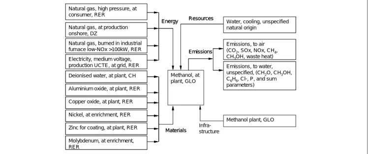
production of 1 kg of methanol (see unit process 'Metha-nol, at plant, GLO', Fig. 1). The unit process 'Methanol plant, GLO' considers the use of land, materials, and en-ergy as well as transport processes and waste treatment. 2. Methanol, at plant, GLO: this dataset describes average
worldwide production of 1 kg pure methanol. This unit process will be presented in detail below.
3. Methanol, at regional storage, CH: This process unit may be useful if methanol is used in Switzerland (CH). In addition to methanol production, transport, storage and losses of methanol are considered. Transport is assessed by determining the various production locations of the methanol used in Switzerland and weighting the respec-tive transport distances with the according methanol amounts from these locations.
The unit process Methanol, at plant, GLO contains inven-tory data about the production of 1 kg of methanol. Since more than 90% of worldwide methanol production is made of natural gas (Fiedler et al. 2001), we only considered this production route. Three technologies and several plant sizes were considered in this inventory. We used data from plant builders (Johnson Matthey), scientific journals (Nitrogen & Methanol), a PhD thesis (Pehnt 2002), and textbooks (Cheng 1994, Häussinger et al. 2000) as literature sources.
The inputs and outputs of the methanol production pro-cess are shown in Fig. 1. Natural gas is needed as feedstock and as an energy source. Furthermore, electricity and wa-ter (cooling and process wawa-ter) are needed, as well as met-als used as catalysts. During methanol production, emis-sions are released to air and water (see Fig. 1). Infrastructure demands are contained in the process unit 'Methanol plant, GLO' (see above).
The main resource needed for methanol production is natu-ral gas. To set up the inventory, first, available data about the natural gas demand of existing plants was collected (Table 1). Since the unit process 'Methanol, at plant, GLO' shall rep-resent worldwide methanol production, an average value was used in the inventory, as well as a maximum and mini-mum value for the uncertainty analysis (last three lines of Table 1). The values presented in technical literature (Le Blanc et al. 1994) were assumed to represent the average for the total natural gas consumption. These values were de-rived from a methanol plant with steam reforming process and an average plant size (2000 tonnes per day). The steam reforming process was chosen as reference because it is the technology most used in the world (60% of the world ca-pacity (Synetix 2000a)). The maximum value was determined from an old methanol plant working with steam reforming Fritsch 2000. As minimum value, we used the natural gas demand of a modern high efficiency combined reforming plant design (Nitrogen and Methanol 2001).
Three different natural gas unit processes were used to de-scribe the resource use of natural gas (see Fig. 1). All these three unit processes consider the complete production chain of natural gas. The two unit processes 'natural gas, high pressure, at consumer, RER' and 'natural gas, at produc-tion, onshore, DZ' were used to describe the fraction of natu-ral gas used as feedstock, while the third unit process 'natu-ral gas, burned in industrial furnace low-NOx>100kW, RER'
(see Fig. 1) was used for the fraction of natural gas used as
Methanol, at plant, GLO
Methanol plant, GLO Emissions, to air (CO2, SOx, NOx, CH4,
CH3OH, waste heat)
Emissions, to water, unspecified, (CH2O, CH3OH, C6H6, Cl-, P, and sum parameters) Emissions Emissions, to air (CO2, SOx, NOx, CH4,
CH3OH, waste heat)
Emissions, to water, unspecified, (CH2O, CH3OH, C6H6, Cl-, P, and sum parameters) Emissions Infra-structure Natural gas, high pressure, at
consumer, RER Natural gas, at production onshore, DZ
Natural gas, burned in industrial furnace low-NOx >100kW, RER
Energy
Electricity, medium voltage, production UCTE, at grid, RER Natural gas, high pressure, at consumer, RER
Natural gas, at production onshore, DZ
Natural gas, burned in industrial furnace low-NOx >100kW, RER
Energy
Electricity, medium voltage, production UCTE, at grid, RER
Resources
Water, cooling, unspecified natural origin
Resources
Water, cooling, unspecified natural origin
Materials Deionised water, at plant, CH
Aluminium oxide, at plant, RER Copper oxide, at plant, RER
Zinc for coating, at plant, RER Molybdenum, at enrichment, RER
Nickel, at enrichment, RER
Materials Deionised water, at plant, CH
Aluminium oxide, at plant, RER Copper oxide, at plant, RER
Zinc for coating, at plant, RER Molybdenum, at enrichment, RER
Nickel, at enrichment, RER Deionised water, at plant, CH Aluminium oxide, at plant, RER Copper oxide, at plant, RER
Zinc for coating, at plant, RER Molybdenum, at enrichment, RER
Nickel, at enrichment, RER
Fig. 1: Process chain for methanol production (unit process 'Methanol, at plant, GLO'). Names in the boxes denote unit processes of the ecoinvent database (RER: Europe, DZ: Algeria, CH: Switzerland, GLO: global)
an energy source. In contrast to the former two processes, the latter considers emissions to air from the combustion of natural gas. The reason for using two different unit pro-cesses for the feedstock-gas was that methanol plants are scattered all over the world (and they are increasingly built at remote locations, where resources of natural gas are avail-able). Therefore, natural gas needs to be transported over long distances at some sites, while no pipeline is needed at other sites. Accordingly, the two unit processes reflect dif-ferences in transport distances.
Other resource demands were determined in a similar way as with respect to natural gas. Emissions to air are domi-nated by the emissions of the furnace. Most air emissions are already included in the unit process 'natural gas, burned in industrial furnace low-NOx>100kW, RER'. However, the methanol synthesis produces access amounts of hydrogen, the burning of which produces thermal NOx emissions. Therefore, the average additional NOx emissions were cal-culated with the NOx emission factor for industrial furnaces
(low-NOx>100kW), as presented in Faist Emmenegger et al. 2003. Moreover, SOx is emitted from desulphurisation of natural gas. It was assumed that all the sulphur entering the unit is released as SO2 during regeneration. VOC
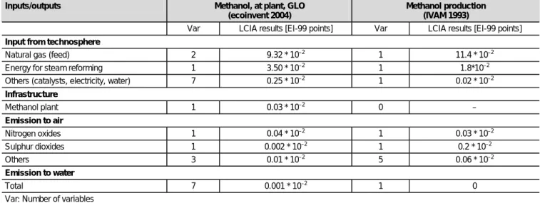
emis-sions from purge vent and the distillation vent were consid-ered using data from technical literature (Delucci et al. 1996). The only emissions to water arise in the purification of metha-nol. Distillation residues containing water, methanol, ethanol, higher alcohols, other oxygen containing compounds, and variable amounts of paraffin, are discharged. This effluent is treated biologically, which was considered in the inventory. Table 2 displays a comparison of the methanol unit process dataset used in ecoinvent with a corresponding dataset from IVAM (Environmental Research University of Amsterdam (IVAM) 1993). For both datasets, the ecoinvent 1.01 (ecoinvent Centre 2003) data was used for the background technosphere flows (see Input from technosphere in Table 2). The reason for this was to compare merely the unit processes without
Flow Process type Plant size [tonnes per day] Total [MJ] Feed [MJ] Fuel [MJ]
2500 36.8 / 38 33.7 / 35.1 3.1 / 2.9 2000 35.8 / 36.3 34.4 / 33.5 1.4 / 2.8 500 39.2 / 40.7 – – Steam reforming Unspecified 37.2 – – 2500 36.1 29.5 2.1 2000 33 / 31.6 31.9 1.1 Combined reforming Unspecified 32.7 – – 5000 31.6 – – 2000 35.3 35.3 –
Natural gas demand (HHV) per kg methanol Autothermal reforming Unspecified 32.1 – – Average value 36.3 33.5 2.8 High value 40.7 37.6 3.1 Low value 31.6 30.5 1.1
Table 1: Natural gas demand for methanol production with three technologies (steam reforming, combined reforming, autothermal reforming), several plant sizes, and values chosen for the ecoinvent unit process 'Methanol, at plant, GLO' (Fitzpatrick 2000, Fritsch 2000, Hydrocarbon Processing 1985, Le Blanc et al. 1994, Nitrogen 1995, Nitrogen and Methanol 2001, Synetix 2000b). The energy demand refers to the gross calorific value (HHV) of natural gas
Inputs/outputs Methanol, at plant, GLO
(ecoinvent 2004)
Methanol production (IVAM 1993)
Var LCIA results [EI-99 points] Var LCIA results [EI-99 points] Input from technosphere
Natural gas (feed) 2 9.32 * 10–2 1 11.4 * 10–2
Energy for steam reforming 1 3.50 * 10–2 1 1.8*10–2
Others (catalysts, electricity, water) 7 0.25 * 10–2 1 0.02 * 10–2
Infrastructure Methanol plant 1 0.03 * 10–2 0 – Emission to air Nitrogen oxides 1 0.04 * 10–2 1 0.03 * 10–2 Sulphur dioxides 1 0.002 * 10–2 1 0.2 * 10–2 Others 3 0.01 * 10–2 5 0.06 * 10–2 Emission to water Total 7 0.001 * 10–2 1 0
Var: Number of variables
Table 2: Comparison of the inventories of production of 1 kg methanol used in the ecoinvent database and in the Simapro extensa database Pré Consultants 2002 (Environmental Research University of Amsterdam (IVAM) 1993). The number of reported inputs and outputs in the datasets is shown in the column 'var'. The LCIA results were calculated using Ecoindicator 99 (H/A) methodology (Goedkoop & Spriensma 2000)
Inputs/outputs Ecoinvent ESU’96 Changes between
Ethylene, average Ethylene, pipline Ethylene two databases
Cumulative Energy Demand (in MJ-Eq per kg ethylene)
non-renewables, fossil 6.69 *101 7.00 *101 7.77 *101 –11.9%
non-renewables, nuclear 4.72 *10–1 3.02 *10–1 1.56 –75.2%
renewables, water 1.90 *10–1 2.31 *10–2 2.21 *10–1 –51.8%
renewables, wind, solar, geothermal 7.99 *10–6 6.42 *10–6 0 –
renewables, biomass 8.21 *10–3 3.08 *10–3 0 –
Air emissions (in kg per kg ethylene)
Carbon monoxide, fossil 8.87 *10–4 1.17 *10–3 9.46 *10–4 +8.7%
Carbon dioxide, fossil 1.16 1.15 1.96 –41.1%
NMVOC 1.70 *10–3 1.21 *10–3 1.33 *10–2 –89.1% Nitrogen oxides 6.35 *10–3 4.74 *10–3 5.17 *10–3 +7.2% Sulphur dioxide 5.16 *10–3 3.22 *10–3 1.41 *10–2 –70.3% Particulates, > 10 um 2.21 *10–4 1.80 *10–4 Particulates, < 10 and > 2.5 um 2.96 *10–4 2.39 *10–4 Particulates, < 2.5 um 1.71 *10–4 1.38 *10–4 1.12 *10–3 –44.4%
Water emissions (in kg per kg ethylene)
BOD 8.43 *10–5 7.75 *10–5 4.30 *10–6 +1861.4%
COD 3.02 *10–4 3.03 *10–4 1.22 *10–4 +146.6%
Chloride 1.53 *10–4 2.34 *10–4 3.28 *10–2 –99.5%
considering differences in the background data. The results show that the feedstock causes the largest environmental impact (see Table 2). The according values of both datasets are in the same order of magnitude. The aggregated envi-ronmental impact of the other technosphere inputs, such as catalysts, electricity and water (see Table 2), are one order of magnitude higher in the ecoinvent dataset, because elec-tricity for rotary machines, compressors, fans, and pumps are considered in ecoinvent, in contrast to the IVAM dataset. Comparing the foreground processes, the two inventories are in reasonable accordance concerning most inventory flows. One exception is the environmental impact of sulphur diox-ide emissions, which are two orders of magnitude higher in the IVAM inventory. Sulphur dioxide emissions originate from the desulphurisation of the natural gas used as feedstock. In the ecoinvent dataset, sulphur dioxide emissions are estimated using an emission factor, which takes into account the vari-able sulphur content of natural gas from different gas mining sites. By contrast, the IVAM dataset focusses on gas mining on the continental shelf (North sea gas fields). Furthermore, and in contrast to the IVAM dataset, the use of catalysts, the discharge of distillation residues, and the use of infrastructure are taken into account in the ecoinvent dataset.
3.2 Cumulative Industry data (APME data): Ethylene case study
One of the most important raw materials for the produc-tion of chemicals is raw oil. Within a typical refinery pro-cess, about 50 to 150 kg of naphtha – the fraction of crude oil with a boiling point between 104 and 157°C (Leffler 1985) – are produced per tonne of raw oil as the starting point for the further processing. Naphtha comprises vari-ous unsaturated hydrocarbon molecules and is therefore only suitable as a raw material for the polymer industry after cracking. This processing step splits naphtha into
smaller, unsaturated and, hence, more reactive molecules, primarily into ethylene, propylene, various butylenes and butadiene. Within these chemicals, ethylene (CAS No. 74-85-1) is the largest-volume petrochemical produced world-wide (Häussinger et al. 2000). However, this chemical is mainly used as an intermediate, e.g. for the production of polyethylene. Due to its importance for the plastics indus-try, inventory data for ethylene have been collected already in an early stage of the LCA history. According to an Aus-tralian review (CRC for Waste Management and Pollution Control 1998), around half a dozen of different datasets for ethylene are published, used in a variety of further da-tabases and documents concerned with LCI data. In Swit-zerland, several of these sources have been used so far – while the ethylene data in the previous Swiss energy sys-tems LCI database (ESU'94, ESU'96) are based on a US-study (Tellus-Institute 1992), the dataset in the previous packaging LCI database (SRU 250) is based on the Euro-pean Plastics data (Boustead 1999). Within the ecoinvent project, the data from APME have been used due to the fact that they are representing best the actual European pro-duction of ethylene. The major drawback of these data is the fact that they are not available on a unit process level, but only as an aggregated and cumulated dataset.
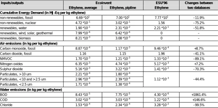
A comparison of the dataset for ethylene integrated into the database ecoinvent with the dataset in the former energy inventories (Frischknecht et al. 1996), based on a US study (Tellus-Institute 1992), is established. In Table 3, selected cumulative inventory results as well as the life cycle impact assessment (LCIA) factor cumulative energy demand are shown for the two data sources mentioned.
Comparing the selected results shown in Table 3, large dif-ferences can be observed. While a clear reduction for the APME data is shown compared to the ESU inventory for
Table 3: Selected cumulative inventory results and the LCIA indicator cumulative energy demand of the production of ethylene (Data sources: Frischknecht et al. 1996, Hischier 2004). The values in the last row show the changes from ESU'96 (Frischknecht et al. 1996) to ecoinvent (Hischier 2004) as difference of the average from the two datasets in ecoinvent and ESU'96, expressed in % of the ESU’96 value
the cumulative energy demand as well as parts of the emis-sions to air, the two inventories differ up to two orders of magnitude in both directions for the water emissions. A more detailed comparison of the two datasets is hardly possible due to the missing transparency in the APME data.
3.3 Estimation based on technical reference source: Propylene glycol case study
A variety of chemical datasets has been established based on the framework described in Section 2.3. One of these chemicals is propylene glycol (CAS No. 57-55-6, HOCH2CH (CH3)OH), an important precursor for the production of unsaturated polyester resins and thus of automotive plas-tics, fibreglass boats and construction materials. Furthermore, it is used as a solvent or as a preservative in food and pet food products, or in the de-icing as well as the lubricant sectors. The only data source available within the framework of the ecoinvent work for propylene glycol was the respective chap-ter from Ullmann's (Sullivan 2000), in which the overall reac-tion for the producreac-tion of this substance is reported as:
CH2OC(CH3)H + H2O → HOCH2CH(CH3)OH (1)
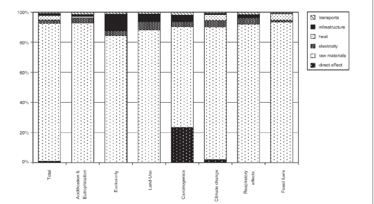
Fig. 2 shows the contribution of process inputs to the results from the cumulative process of propylene glycol. The LCIA method applied here is the Eco-indicator'99, hierarchist per-spective, of which the total score as well as several indi-vidual impact scores are shown.
As can be seen in Fig. 2, the raw materials dominate the impact score, while the contribution from all other process inputs is very small. However, this is not really astonishing due to the fact that the only input that is not based on as-sumptions but on the stoichiometric equation documented in Sullivan (2000) is raw material input. The amounts of direct emissions as well as the energy consumption, by con-trast, are very rough estimations, and waste production is completely neglected. While, with respect to direct emissions and energy, other amounts as well as further types of emis-sions are possible in reality, resulting in either an increase or decrease in the environmental load, more information on the amount and type of waste generated can only result in a higher environmental load.
To conclude, a dataset such as propylene glycol can only be used in a life cycle assessment study when the respective chemical substance is not a crucial part of the problem set-ting of the study. A comparison with older inventory data of this substance is not possible, as no such inventory has been established in the past.
4 Summary, Discussion, and Outlook
The present paper illustrates various methods that were used in the context of the ecoinvent database to establish LCIs of chemicals in situations of differing data availability. With the help of these approaches, more than 200 datasets of important chemicals were included in the ecoinvent data-base. This constitutes a major progress in LCI development
Fig. 2: Contribution of process inputs to the cumulative impact of 1 kg of propylene glycol, expressed as several impact scores from the Eco-Indicator'99 methodology
of chemicals, which traditionally has been characterized by limited data availability.
The three procedures presented in this paper illustrate how LCI data of basic chemicals were established in ecoinvent. As a first priority, the general guidelines of ecoinvent were followed to set up the inventories. This procedure could be followed with respect to some chemicals, such as illustrated with the case study of methanol. The comparison of the ecoinvent dataset with the IVAM dataset showed that the ecoinvent dataset is able to cover the methanol production process in more detail. Unfortunately, such a good data situ-ation is rare with respect to chemicals. As a second priority, data from the APME were therefore used within ecoinvent. These data have the advantage of representing well average European production conditions (covering up to 100% of the production in mid to end nineties of the last century). However, major drawbacks are that these datasets are not in accordance with the ecoinvent philosophy of a unit pro-cess database (see Frischknecht et al. 2004b). The main dis-advantage from this is that no information on the different production steps is available, and thus it is not possible to make any statement on which process step or input material contribute most to the environmental impact of chemicals, such as presented in the case study of ethylene. A further problem is the fact that these datasets are not based on the same preceding process steps as the other data in ecoinvent. For instance, the APME data are based on their own elec-tricity mix model. These differences allow no direct com-parison of the APME data with other ecoinvent data. In brief, APME datasets do not allow one to fully achieve one primary aim of the project ecoinvent – the harmonization of the various LCI datasets.
If no information was available at all from the literature, the third procedure was followed, namely using the stoichio-metric reaction equation as only an information input. While this is a rather crude procedure, it represents one way how to consider the vast majority of existing chemicals within ecoinvent, namely chemicals of which only basic process information is available. This procedure therefore represents an alternative to neglecting chemicals in LCA. Since the pro-cedure uses only very little information as input informa-tion, it can potentially be applied to many more chemicals than has been done in the current version of ecoinvent. One major drawback of this procedure, however, is that the esti-mations of LCI data are very uncertain and that there is a high risk involved that important aspects of the life-cycle are not considered. To conclude, a dataset that was estab-lished on the basis of the overall reaction equation, such as presented in the case study of propylene glycol, can only be used in a life cycle assessment study when the respective chemical substance is assumed not to be a crucial part of the problem setting of the study.
One of the goals of the ecoinvent project was to provide harmonized and transparent data on a unit process level. With respect to chemicals, these aims could only be partly fulfilled. The major reason was the extremely heterogeneous
availability and quality of chemical LCI data. In order to harmonize the data, the methods and procedures presented in this paper were developed and applied within the ecoinvent project. These approaches were successful in transforming the data into a common format and, thus, they enabled the consideration of a large number of chemi-cals. This is a major advance in the field of chemical LCI data. However, the inventory data of chemicals in ecoinvent is far from being complete, and some of the data included in ecoinvent does not meet the quality goals of ecoinvent. This is especially the case for the data elaborated according to the second and partly to the third approach described above. One of the aims for future versions of the ecoinvent database is therefore to establish more sound inventories for all those chemical substances not yet inventoried ac-cording to the first approach described within this paper. Besides the improvement of already established inventories, the compilation of further harmonized inventories of spe-cific types of chemicals (e.g. solvents) or of chemicals for new industrial sectors (e.g. electronics industry) are in dis-cussion. International bodies such as OECD and EU have recognized the need for more documentation of chemical ingredients, and corresponding activities are currently un-dertaken to stimulate information exchange and documen-tation on the contents of chemicals in products. Such infor-mation will facilitate LCI work with respect to chemicals included in products, i.e. it will help to identify chemicals that are of high priority and need to be included in LCI databases such as ecoinvent.
With regard to the LCIA results of many chemicals in ecoinvent, environmental impacts related to energy demand are often of primary importance. However, this may be due to the fact that information about chemical emissions is not complete. For instance, from approximately 100,000 exist-ing chemicals, there are only a few hundred chemicals for which LCIA characterization factors exist. This situation is likely to improve in the future. For instance, databases, such as the SIDS (Screening Information Data Set) database of OECD (OECD 2003), are currently set up that aim to in-clude substance property data of chemicals for a large vari-ety of chemicals. These developments may help to consider more chemical emissions in future LCIA methods, which would have according implications on the inventory side (reporting and recording of the releases of these chemicals in manufacturing and use).
References
Althaus H-J, Chudacoff M, Hischier R, Jungbluth N, Osses M, Primas A (2004): Life Cycle Inventories of Chemicals. CD-ROM, No. Final report ecoinvent 2000 No. 8, EMPA Düben-dorf, Swiss Centre for Life Cycle Inventories <http://www. ecoinvent.ch>, Dübendorf, CH
Boustead I (1993): Eco-Profiles of the European Plastics Industry. Olefin feedstock sources. No. Report 2, Association of Plas-tics Manufacturers in Europe (APME) <http://www.apme. org/lca, Brussels>
Boustead I (1994): Eco-profiles of the European polymer indus-try. Co-Product Allocation in Chlorine Plants. No. Report 5, Association of Plastics Manufacturers in Europe (APME), Brussels
Boustead I (1999): Eco-Profiles of Plastics and Related Intermedi-ates. Methodology. Association of Plastics Manufacturers in Europe (APME) <http://www.apme.org/lca>, Brussels Cheng WH (1994): Methanol Production and Use. Marcel Dekker
Inc., New York
CRC for Waste Management and Pollution Control (1998): Life Cycle Inventory of Polyethylene Manufacture in Australia. Draft report Centre for Design at RMIT, Melbourne
Delucci M, Wang Q, Ceerla R (1996): Emissions of criteria pollut-ants, toxic air pollutants and greenhouse gases from the use of alternative transportation modes and fuels. UCD-ITS-RR-96-12 1. Institute of Transportation Studies. University of Califor-nia <http://www.uctc.net/papers/344.pdf>, Davis (CA) ecoinvent Centre (2003): ecoinvent data v1.01. CD-ROM No.
ISBN 3-905594-38-2, Swiss Centre for Life Cycle Inventories <http://www.ecoinvent.ch>, Dübendorf, CH
Environmental Research University of Amsterdam (IVAM) (1993): Methanol production in Simapro extensa database
Faist Emmenegger M, Heck T, Jungbluth N (2003): Erdgas. In: Dones R (ed), Sachbilanzen von Energiesystemen: Grundlagen für den ökologischen Vergleich von Energiesystemen und den Einbezug von Energiesystemen in Ökobilanzen für die Schweiz. Paul Scherrer Institut Villigen, Swiss Centre for Life Cycle In-ventories, Dübendorf, CH
Fiedler E, Grossmann G, Kersebohm D, Weiss G, Witte C (eds) (2001): Methanol, Chapter 4,6,8,10. In: Ullmann's Encyclope-dia of Industrial Chemistry, Sixth Edition, June-2001 Electronic Release. Wiley InterScience <http://www.mrw.interscience.wiley. com/ueic/ull_search_fs.html>, New York
Fitzpatrick TJ (2000): Impact of New Technology on Methanol Plant Production Costs. IMTOF 99 Paper 596W/029/0/IMTOF. Synetix (ICI Group), Cleveland (UK)
Frischknecht R, Bollens U, Bosshart S, Ciot M, Ciseri L, Doka G, Dones R, Gantner U, Hischier R, Martin A (1996): Ökoinven-tare von Energiesystemen. ESU-Schlussbericht ETH/PSI, Zürich/ Villigen
Frischknecht R, Jungbluth N, Althaus H-J, Doka G, Dones R, Heck T, Hellweg S, Heck T, Hischier R, Nemecek T, Rebitzer G, Spielmann M (2004a): The ecoinvent Database: Overview and Methodological Framework. Int J LCA 10 (1) 3–9 Frischknecht R, Jungbluth N, Althaus H-J, Doka G, Dones R,
Hischier R, Hellweg S, Nemecek T, Rebitzer G, Spielmann M (2004b): Overview and Methodology. CD-ROM Final report ecoinvent 2000 No. 1, Swiss Centre for Life Cycle Inventories <http://www.ecoinvent.ch>, Dübendorf, CH
Fritsch S (2000): Revamp of ENIP Methanol Plant in Algeria. Krupp Uhde GmbH. IMTOF 99 Paper 600W/029/0/IMTOF, Synetix (ICI Group), Cleveland (UK)
Geisler G, Hofstetter TB, Hungerbühler K (2004): Production of Fine and Speciality Chemicals: Procedure for the Estimation of LCIs. Int J LCA 9 (2) 101–113
Gendorf (2000): Umwelterklärung 2000, Werk Gendorf. Werk Gendorf, Burgkirchen
Goedkoop M, Spriensma R (2000): Eco-Indicator '99 Methodol-ogy Report. 2nd ed. pré-Consultants. Amersfoort, Netherlands Häussinger P, Leitgeb P, Schmücker B (eds) (2000): Ullmann's En-cyclopedia of Industrial Chemistry, Sixth Edition, June 2001 Electronic Release. Wiley InterScience <http://www.mrw. interscience.wiley.com/ueic/ull_search_fs.html>, New York Hischier R (2004): Life Cycle Inventories of Packaging and
Graphical Paper. CD-ROM, No. Final report ecoinvent 2000 No. 11, EMPA St. Gallen, Swiss Centre for Life Cycle Inven-tories <http://www.ecoinvent.ch>, Dübendorf, CH
Hydrocarbon Processing (1985): Petrochemical Processes, Spe-cial Report, November 1985. Hydrocarbon Processing 64 (11) 144–146
Jansen B (2002): Consolidating a culture of risk prevention. In: Dangerous substances – Handle with care. European Agency for Safety and Health at Work (6) 4–5
Jimenez-Gonzales C, Kim S, Overcash MR (2000): Methodology for Developing Gate-to-Gate Life Cycle Inventory Information. Int J LCA 5 (3) 153–159
Le Blanc JR, Schneider RV, Ill and Strait RB (1994): Production of Methanol. In: Cheng WH (ed), Methanol Production and Use. Vol. 1 , pp 51–132, Marcel Dekker Inc, New York Methanol (2000): World Methanol Supply / Demand. Source:
DeWitt & Company, Place
Nitrogen (1995): Refining Reforming Technology. In: Nitrogen, Vol. 214 (March/April 1995) 38–56
Nitrogen and Methanol (2001): Mega-methanol and what to use it for. In: Nitrogen & Methanol, Vol. 254 (November/Decem-ber 2001) 24–27
OECD (2003): OECD's environment, health and safety pro-gramme brochure. OECD Environment Directorate Environ-ment, Health and Safety Division, Paris
Pehnt M (2002): Ganzheitliche Bilanzierung von Brennstoffzellen als zukünftige Energiesysteme. In: Fortschrittsberichte Vol. 6 (476)
Pré Consultants BV (2002): Simapro 5.0 LCI Database and LCA Software, Amersfoort, Netherlands
Sullivan CJ (2000): Propanediols. In: Häussinger P, Leitgeb P, Schmücker B (eds), Ullmann's Encyclopedia of Industrial Chem-istry, Sixth Edition, June-2001 Electronic Release. Wiley InterScience, New York
Synetix (2000a): Methanol Plant Technology. ICI Leading Con-cept Methanol (LCM) Process, 2002, Place
Synetix (2000b): Methanol Plant Technology. ICI Low Pressure Methanol (LPM) Process, 2002, Place
Tellus-Institute (1992): Impacts of production and disposal of pack-aging materials – Methods and case studies. Tellus-Institute, Boston, MA (USA)
Received: July 18th, 2004 Accepted: October 24th, 2004 OnlineFirst: October 25th, 2004