HAL Id: hal-01111966
https://hal.inria.fr/hal-01111966
Submitted on 2 Feb 2015
HAL is a multi-disciplinary open access
archive for the deposit and dissemination of
sci-entific research documents, whether they are
pub-lished or not. The documents may come from
teaching and research institutions in France or
abroad, or from public or private research centers.
L’archive ouverte pluridisciplinaire HAL, est
destinée au dépôt et à la diffusion de documents
scientifiques de niveau recherche, publiés ou non,
émanant des établissements d’enseignement et de
recherche français ou étrangers, des laboratoires
publics ou privés.
Jean-Baptiste Apoung-Kamga, Pascal Have, Jean Houot, Michel Kern, Adrien
Semin
To cite this version:
Jean-Baptiste Apoung-Kamga, Pascal Have, Jean Houot, Michel Kern, Adrien Semin. Reactive
Trans-port in Porous Media. ESAIM: Proceedings, EDP Sciences, 2009, CEMRACS 2008 - Modelling and
Numerical Simulation of Complex Fluids, 28, pp.227 - 245. �10.1051/proc/2009049�. �hal-01111966�
Editors: Will be set by the publisher
REACTIVE TRANSPORT IN POROUS MEDIA
∗Jean-Baptiste APOUNG
1, Pascal HAVE
2, Jean HOUOT
3, Michel KERN
4and
Adrien SEMIN
5Abstract. We present a numerical method for coupling transport with chemistry in porous media. Our method is based on a fixed-point algorithm that enables us to coupled different transport and chemistry modules. We present the methods for solving the sub-problems, detail the formulation for the coupled problem and show numerical examples to validate the method.
Résumé. Nous présentons une méthode numérique pour le couplage du transport et de la chimie en milieu poreux. Notre méthode utilise un algorithme de point fixe, qui nous permet de coupler des modules de transport et de chimie différents. Nous présentons les méthodes numériques utilisées pour chacun des sous-problèmes, ainsi qu’une formulation pour le problème couplé, et nous validons la méthode sur quelques exemples numériques.
Introduction
Most of our drinking water comes from underground resources, but these resources are subject to numerous threats of various origins: industrial and agricultural waste, acid rains, nuclear waste, ... Understanding these risks to mitigate them, and implement remediation policies if possible, is becoming an increasingly important stake [34]. In this respect, chemical phenomena play a fundamental role: chemical species in the subsurface may react both between themselves,to form new compound species, and also with the host rock. These heteroge-neous reactions could potentially have an important effect on the flow and transport phenomena, by opening new channels, or closing existing ones. The mathematical model underlying these phenomena couples a transport model (advection–diffusion partial differential equations) together with a chemical model (ordinary differential equations or algebraic equations, depending on whether chemistry is modeled with kinetic or equilibrium reac-tions).
This work is concerned with a numerical method for the simulation of coupled transport–chemistry models. We consider a simplified setting, with only equilibrium reactions, and we only take into account heterogeneous reac-tions in the form of sorption. The transport–chemistry problem thus takes the form of a large system of PDEs coupled with algebraic equations. As the numerical methods for both parts of the system are quite different, we
∗This work was supported by ANR SHPCO2 project, and partly supported by Groupement MoMaS (PACEN/CNRS, ANDRA,
BRGM, CEA, EdF, IRSN)
1 Laboratoire de mathématiques, Université Paris-Sud, [email protected] 2 IFP, [email protected]
3 Institut Elie Cartan, Nancy, [email protected]
4 INRIA Paris-Rocquencourt, Equipe-projet ESTIME, [email protected] 5 INRIA Paris-Rocquencourt, Equipe-projet POems, [email protected]
c
want the overall coupling algorithm to respect this separation (see [37] for a discussion of various approaches to reactive transport simulation). In this work we use a simple fixed–point algorithm [16, 24, 31], that enables us to put together the pieces for a general coupling strategy, and to demonstrate some of the phenomena involved. An outline of the paper is as follows: in section 1 we present the models used for the basic phenomena of flow transport and chemistry. The solution method, both for the individual sub-problems and for the overall coupled problem are presented in section 2, and we show numerical examples in section 3.
1. Presentation of the flow, chemical phenomena and transport
We consider a porous medium occupying a domain Ω⊂ Rd (d = 2 or 3) and carrying a set of chemical species
that can either be in solution (aqueous species) or attached to the host rock matrix (sorbed species). The 3 main phenomena we describe are the flow of water in the subsurface (we assume the flow is stationary, and that there is no feedback between chemistry and flow), the transport of the various species, due to this flow, and chemical phenomena both between species in solution, and between the species and the host matrix.
1.1. Flow phenomena
We consider Darcy’s law and the incompressibility law to describe the velocity u and the pressure p of the flux
in the domain Ω : {
ωu = −K∇p
∇ · (ωu) = 0 in Ω, (1)
where ω is the porosity of the medium (expressing the amount of void in the porous medium), and K is the permeability tensor. The boundary conditions may be of different type
{
p = p0 on ΓD,
u.n = g on ΓN,
, (2)
with p0 a given boundary pressure, and g a prescribed boundary flux. We assume that the Darcy velocity is
not affected by the chemical phenomena (i.e. flow is constant over time, and the porosity does not depend on the concentrations of the various species). We make the usual assumptions on the permeability K, which may be a tensor, and may depend on x : we assume that K ∈ L∞(Ω)d×dand that there exists constants k∗ and k∗ such that,
∀ξ ∈ Rd, 0 < k
∗|ξ|2≤ ξTKξ≤ k∗|ξ|2<∞.
We also assume that the functions p0and g are “smooth enough”.
1.2. Chemical reactions
We assume that the chemical reactions are local (that is, we consider that the reaction phenomena at a point
x∈ Ω only involve the concentrations of the species at this point). According to Rubin [30], chemical reactions
can be classified according as to whether they are kinetic or at equilibrium, and whether they are homogeneous or heterogeneous. In this work, we only consider instantaneous reactions (there is no kinetic term), and only some forms of heterogeneous reactions.
The restriction to equilibrium only reactions deserves some justification. This is a common modelling hypoth-esis in reactive transport in porous media (see for instance the discussions in Valocchi [35] or Rubin [30]). Its validity stems from the fact that chemical phenomena usually occur on a much faster time scale than the transport phenomena, thus leading to the so-called “local equilibrium” assumption (this is of course in sharp contrast with the situation in atmospheric chemistry where taking into account kinetic reactions is essential, see for instance [3]). For the kind of applications discussed in this paper, kinetic models would be needed if we had included minerals, or biodegradation reactions. Finally, we briefly indicate at the end of section 1.4 the modifications that would be necessary if we took kinetic reactions into account.
As to the nature of the reactions, it is customary to distinguish between two types of chemical reactions: Homogeneous reactions: These occur only within the aqueous phase, and include for instance,
com-plexation, acid–base reactions, and oxydo–reduction reactions;
Heterogeneous reactions: These obviously play a fundamental role in geochemistry. They include precipitation dissolution reactions, whereby an aqueous species can form a solid complex. These are threshold reactions, with specific difficulties, and we do not consider them further in this paper. The other type of heterogeneous reactions are the sorption reactions, which are the main vehicle of exchange at the rock–water interface. We only consider a ion–exchange mechanism, where ions are exchanged between the aqueous species and the rock matrix, and a complex is formed on the matrix. Only a specific number of “sites” on the matrix can accept ions. The medium is characterized by its Cationic Exchange Capacity (CEC). More details on the actual mechanisms involved can be found in the reference book [12]. From the simplified point of view adopted in this paper, the end result is that we can model sorption reactions in the same way as homogeneous ones.
Note that the equilibrium assumption is consistent with the restriction to sorption reactions only.
We now consider NA aqueous species and NS sorbed species, undergoing NR linearly independent chemical
reactions that can be written as
NA∑+NS
j=1
AijEj ⇆ 0, i = 1, . . . , NR.
We can express NR species, that we call secondary species, according to the Morel formalism (see [25]), as
functions of the NP = NA+ NS− NR other species, that we call primary species.
In the following, we denote by X1, . . . , XNxthe concentrations of the primary aqueous species and by Y1, . . . , YNy
the concentrations of the primary sorbed species (note that Nx+ Ny = NP). In the same way, we denote by
C1, . . . , CMc the concentrations of the secondary aqueous species and by S1, . . . , SMs the concentrations of the
secondary sorbed species (note also that Mc+ Ms= NR). Of course these concentrations are functions defined
onRt× Ω.
To describe the chemical problem, we have two types of laws to consider :
Mass Action Law : Each reaction gives rise to a mass action law, describing how we can get the concentrations of the secondary species, given the concentrations of the primary species.
Mass action law for aqueous species : since we consider no precipitation phenomena, the ithsecondary aqueous specie is obtained from a linear combination of the Nxprimary aqueous species. Denote byA1,i,j the coefficient
of the jth primary aqueous specie in this linear combination. The mass action law can then be written, in
logarithmic form, as
log(Ci) = Nx
∑
j=1
A1,i,jlog(Xj) + log(KCi) (3)
where KCi is a thermodynamic constant which depends only on the temperature (supposed constant in our
model).
Mass action law for sorbed species : in the same way, the ith secondary sorbed specie is obtained from a linear
combination of the Nx primary aqueous species (with linear coefficients A3,i,j) and the Ny primary sorbed
species (with linear coefficientsA4,i,j). The mass action law can be written as
log(Si) = Nx ∑ j=1 A3,i,jlog(Xj) + Ny ∑ j=1
where KSi is a thermodynamic constant which depends only on the temperature.
Conservation Law : the Conservation Law (also known as the Lavoisier law) can be expressed by the two following relations Ti= Mc ∑ j=1 A1,j,iCj+ Ms ∑ j=1 A3,j,iSj+ Xi, ∀i ∈ {1, . . . , Nx} (5) Wi = Ms ∑ j=1 A4,j,iSj+ Yi, ∀i ∈ {1, . . . , Ny} (6)
where Ti is the total concentration of the aqueous specie Xi and Wi is the total concentration (related to the
CEC of the medium, and assumed constant over time in our model) of the sorbed specie Yi.
Summary : if we denoteAk the matrix with coefficients Ak,i,j, the Mass Action Laws (3, 4) and the
Conser-vation Law (5, 6) can be put in the following matrix form [ log(C) log(S) ] = [ A 1 0 A3 A4 ] [ log(X) log(Y ) ] + [ log(KC) log(KS) ] and [ T W ] = [ AT 1 A T 3 0 AT4 ] [ C S ] + [ X Y ] (7)
where log(Z) is the vector whose ith component is equal to log(Z
i).
We can summarize these matrix equations by giving the Morel tableau:
X Y K
C A1 0 KC
S A3 A4 KS
T W
(8)
This table can be easily found in the literature for concrete examples (see for example the Morel tableau given by (24)).
In the following, for each aqueous species i, we denote by Qi =
∑
A1,j,iCj+ Xiits total aqueous concentration,
and by Fi =
∑
A3,j,iSj its total fixed concentration. The associated matrix forms are Q = AT1C + X and F =AT
3S. Of course one has T = Q + F .
Remark 1.1. If the secondary species are only sorbed species (i.e. Mc = 0), one can easily see that the total
aqueous concentration Qi of each specie i is equal to its concentration Xi.
1.3. Transport model
Since we study the transport of small particles, the mathematical model is the advection-dispersion equation (for any specie Xi, Yi, Ci and / or Si) :
ωdZ
dt +∇ · (ωuZ − D(u)∇Z) = f(Z) in Ω (for aqueous species), (9) or (as only aqueous species are subject to transport)
ωdZ
dt = f (Z) in Ω (for fixed species) (10)
where D(u) is a dispersion tensor given by D(u) = ωdeI + αTω|u| + (αL− αT)ω(u⊗ u)|u|−1 (the Scheidegger
The scalar de is called the molecular diffusion coefficient, αT is the transverse dispersion coefficient and αL
is the longitudinal dispersion coefficient (dispersion is a macroscopic way of taking into account microscopic heterogeneities of the velocity). In practice, we often consider either molecular diffusion only or dispersion only. The boundary conditions can be either of Dirichlet (given concentration), total flux or diffusive flux given. In the sequel, we denote the transport operator by L(Z) =∇ · (ωuZ − D(u)∇Z).
1.4. The coupled system
We make the classical assumption that the diffusion (and dispersivity) coefficients are the same for all species, so that the transport operator is the same. Its validity is at best questionable, but without this assumption, it would be difficult to carry out the reduction to total concentrations.
We write one equation like (9) above for each aqueous primary and secondary species, and one equation like (10) for each fixed species. Each equation involves an unknown reaction term. In order to eliminate these terms, we introduce the total aqueous concentration Q and total fixed concentration F (details on the elimination procedure are given for example in [37]). We obtain a transport equation of the same form for the total aqueous concentration, with a source term given by the (change in) total fixed concentration.
ωdQ
dt + ω dF
dt + L(Q) = 0 with L(Q) =∇ · (ωuQ − D(u)∇Q) (11)
This model is consistent with the model often used for the transport of a single species undergoing sorption (see for example [20]).
Finally, the transport-reaction equations can be written in the form : find C, X, S, Y , Q, F and T defined on Rt× Ω such that : [ log(C) log(S) ] =A [ log(X) log(Y ) ] + [ log(KC) log(KS) ] [ T W ] =AT [ C S ] + [ X Y ] T = Q + F, Q = X +AT 1C, F =AT3S (12) ωdQ dt + ω dF dt + L(Q) = 0 Initial and boundary conditions
(13)
It has recently been shown by S. Kraütle [17] that this system is well posed, under quite general hypotheses on the data.
Let us note that if we had included kinetic reactions in the model, equation (13) would have a zeroth order term, depending on the concentrations of all species, whereas equations (12) would remain intact (including only equilibrium species). Thus most of our work would remain valid, the main difference being that the various transport operators would no longer be uncoupled.
2. Solution algorithms
In the following, we will denote by ∆t the time step (taken constant for simplicity. Variable time step could, and should,easily be included in the framework), and we wish to compute an approximation of the functions F ,
2.1. Solution of the individual problems
2.1.1. Flow solver
The flow computation is not the main focus of this work, but the Darcy velocity is needed for the transport. In a complex geometry, it will not be possible to prescribe a consistent velocity, so we must first compute the flow, where the main unknown will be the velocity, and not the pressure.
It has long been recognized that standard Lagrange finite elements are not adequate for this task (see [26], [11], as the computed flux may not be continuous across a face. The standard method is the mixed finite element, based for instance on the Raviart-Thomas, or Brezzi-Douglas-Marini, spaces (see [5] or [29] for more details about those spaces).
We briefly review the solution of the flow problem (1) by the mixed finite element method. It is based on the mixed formulation of the system: Find (p, u)∈ L2(Ω)× Vg such that :
∫ Ω K−1u.v dx− ∫ Ω p∇.v dx = − ∫ ΓD p0v.n dγ, ∀v ∈ V0 − ∫ Ω q∇.u dx = 0, ∀q ∈ L2(Ω), (14)
where we have defined
Vg= HNg(div, Ω) ={u ∈ L2(Ω),∇.u ∈ L2(Ω), u.n = g on ΓN}.
Existence and uniqueness for the mixed problem (14) follows from the LBB theory (see [5, 29]), thanks to the assumptions on the data made in section 1.1.
For the discretization, we introduce a regular triangulation Th of Ω, where the elements may be triangles or
rectangles in 2D, and tetrahedra or hexahedra in 3D. In the sequel, we concentrate on the rectangular case, as that is what we use in the examples. In order to obtain a positive definite linear system, we will use the hybrid form of the mixed finite element method. We first define the local Raviart-Thomas space, noting that other choices exist [5, 29]. Denoting by K a rectangle in the triangulation, we define
RT0(K) ={vh= ( α + ax β + by ) , (a, b, α, β)∈ R4}. (15) 0 1 00 00 11 11 00 11 00 11
w
3w
4E
1w
2w
1E
2E
3E
4 1q
q
2q
3q
4The degrees of freedom are the fluxes across the side of the elements
λe=
∫
e
vh.ν dγ, for each side e⊂ ∂K,
this is illustrated on figure 1.
Next, we introduce the global spaces:
Vhg ={vh∈ Vg,∀K ∈ Th, vh|K ∈ RT0(K)}, Wh={qh∈ L2(Ω), qh|KP0(K)},
as well as a multiplier space
Λh= ∪ K∈Th {vh.νK, vh∈ RT0(K)}, and Λ p0 h ={λh∈ Λh, ∫ ΓD (λh− p0)µh= 0,∀µh∈ Λh}
where νK is the outgoing normal to K, and the trace is taken in the weak sense.
The mixed hybrid finite element method is obtained by relaxing the inter-element continuity for the normal fluxes, and introducing a Lagrange multiplier. Thus we look for a triple
(ph, uh, λh)∈ Wh× V g h × Λ p0 h such that ∑ K∈Th (∫ K K−1uh.vhdx− ∫ K ph∇.vhdx + ∫ ∂K λhvh.n dγ, ) = 0 ∀vh∈ Vh ∑ K∈Th − ∫ K qh∇.uhdx = 0, ∀qh∈ Wh, ∑ K∈Th ∫ ∂K µhuh.ν dγ = 0 ∀µh∈ Λ0h. (16)
The main advantage of the hybrid method is that both the pressure and the fluxes can be eliminated locally (this was the motivation for relaxing the continuity of the fluxes). Then one obtains a linear system involving only the Lagrange multipliers, which can be interpreted as pressure traces on the edges. It can be shown that this linear system is symmetric and positive definite, so that efficient solution methods can be used.
It is known that the method just described is convergent, ans it has been demonstrated that it can be used for porous media, and that is gives an accurate velocity field, see the above references.
2.1.2. Chemical solver
Due to the widely different orders of magnitude of the concentrations that are commonly encountered (this will be seen in section 3.1 below, for the MoMaS benchmark [23], or the gallic acid example [4]), we solve this system by taking as unknown x = log(X) and y = log(Y ). This has the added advantage that the concentrations X and Y are automatically positive (however Q and F are not necessarily positive), and has become the standard way to solve the problem (see [36] for more details).
If we rewrite our chemical system (12) in terms of the new unknowns x and y, we get [ log(C) log(S) ] = A [ x y ] + [ log(KC) log(KS) ] [ T W ] = AT [ C S ] + [ exp(x) exp(y) ]
that can be rewritten as ATexp ( A [ x y ] + [ log(KC) log(KS) ]) + [ exp(x) exp(y) ] − [ T W ] = 0 (17)
The chemical system (12) can be now seen as searching for a root of the function defined in (17).
Numerically, our chemical solver uses the GSL library1 (see for instance or [14]) and KNM library 2. The chemical solver can use either Newton’s method, Newton’s method with a finite difference Jacobian, Broyden’s method, and the hybridj algorithm (which is a modified version of Powell’s Hybrid method, see [28] or the references given for GSL). Due to the way the code is written, user defined algorithm could easily be integrated. As we have seen above (equation (12)), in the context of reactive transport what is of interest is not so much the individual concentrations, but the way they are distributed between their aqueous part Q and their fixed part F . Accordingly, after system (17) has been solved, we compute F as in equation (12):
F = AT3exp(A3log(X) + A4log(Y )).
To formulate the coupled problem, it will be convenient to condense the solution of the chemical sub-problem by the function ΨC defined as
F = ΨC(T ). (18)
It should be emphasized that the function ΨCis defined implicitly, via the solution of the nonlinear system (17).
Also, we have omitted the dependence on W as, in this work, it is assumed constant in time. The “role” of the function ΨC is thus to take a given total concentration, and to extract its fixed concentration, according to the
chemical equilibrium, This will enable us to treat the chemical solver as a black-box. 2.1.3. Transport solver
We want to be able to couple different transport modules. To achieve this goal, we will formulate the result of a transport step in a way analogous to the chemical solver in section 2.1.2. We write the transport problem, after discretization in space as
dZ
dt + L(Z) = r,
where r takes into account sources and boundary conditions. We assume that the result of a transport step (after discretization both in time and space) can be put in the form
Zn+1= ΨT(Zn, rn, rn+1).
For instance, if we use a method of lines type of discretization, with a backward Euler scheme in time, we obtain
Zn+1= (I + ∆tL)−1(Zn+ ∆trn+1).
The coupling algorithm in section 2.3 will only use the existence of the function ΨT, not its specific form.
To be specific, we now give the details for the discretization of the transport step used in this work. Rather than the full backward Euler time discretization shown above, we use a splitting technique developed by Siegel et
al. [33] (see also [22]), that enables us to use different spatial and temporal approximations for different transport
processes (advection and diffusion). As explained in these references, it is important to be able to use different methods for the discretization of the different phenomena involved in the transport operator. Explicit methods are better suited for dealing with advection type phenomena (implicit methods add more numerical diffusion than explicit ones), whereas diffusion phenomena require an implicit method to overcome the stringent stability restriction of explicit ones.
1GSL : http://www.gnu.org/software/gsl/
The method is based on operator splitting: each time step has an (explicit) advection half-step, followed by an (implicit) diffusion half-step. We first solve, by an explicit method
Zn+1/2− Zn ∆t +∇.(ωuZ n) = 0 in Ω (19) Then we solve Zn+1− Zn+1./2 ∆t − ∇.(D(u)∇Z n+1) = 0, in Ω. (20)
Let us detail each half-step:
Advection step: We discretize equation (19) by an upwind, cell-centered finite volume method. We denote by ¯ZK the average of the concentration over grid cell K. We integrate the equation over a grid
cell K, and use Green’s formula to obtain
|K|Z¯ n+1/2 K − ¯Z n K ∆t + ∫ ∂K ω u.n ZKindγ = 0,
where ZKin is the upwind concentration across the boundary of the cell K. Across one face F = ¯K∪ ¯K′, the upwind concentration is defined by
ZKin= ZKn if u.nF > 0 Zn
K′ if u, n≤ 0 and face F is not a Dirichlet face,
ZdF if face F is a Dirichlet face.
Diffusion step: We use the same mixed finite element method as for the flow problem in section 2.1.1. Indeed, the diffusion half-step can be written in the form
¯ ZKn+1− ¯ZKn+1/2 ∆t +∇.j = 0 j =−D(u)∇ ¯ZKn+1. in Ω,
which has the same form as (14) above, up to the zeroth order term ¯ZKn+1/2, and this can easily be included in a mixed formulation.
The explicit advection step has a CFL restriction that takes the form
∆t≤ min
K
ω|K|
max{K,u.n<0 on ∂K}(UK, 0)
. (21)
A further refinement is to take several advection steps per diffusion step, by choosing a large diffusion time step, and restricting the advection time step to obey the CFL limit given in (21).
When we apply this solution method to the coupled problem (13), the unknown function is Qn+1, and the right hand side r depends on boundary conditions (known) and both Fn (known) and Fn+1(unknown in principle,
but given in the context of a fixed point algorithm). It will be convenient to abuse notation, and to denote the solution of the transport step for equation (13) by
Of course the function ΨT used in (22) may depend on n.
The code for implementing both the flow solver described in section 2.1.1 and the transport solver described here is based on a the LiveV finite element library3.
2.2. Solution of the coupled system by a fixed point method
We recall the definition of ΨC(18) and ΨT (22), and add the relation T = Q + F to obtain the discrete coupled
system Qn+1 = ΨT(Fn+1) Tn+1 = Qn+1+ Fn+1 Fn+1 = ΨC(Tn+1) (23)
This system can be solved by various methods. The classical way is still based on a fixed-point method [37] or [16]. Recently, more global approaches have been used with good success, based on variants of Newton’s method. Several papers implementing global methods are [1, 8, 15, 18, 19]. The paper [9] explains why the so called fixed-point method should more properly be viewed as a Block Gauss-Seidel method.
In this work, we will present results for a fixed-point method, as this has the same ingredient as the more tightly coupled methods, and provides a base case for validating the latter methods. The main advantage of the fixed point method is that the sub-problems ΨT and ΨC are decoupled, and this lets us reuse the solvers for the
sub-problems that we detailed earlier, namely the chemistry solver described in section 2.1.2, and the transport solver described in section 2.1.3.
We note that a Newton–Krylov method for solving the coupled problem (23) is currently being implemented. In this method, the nonlinear system (23) is solved by Newton’s method, and the linear system arising at each Newton iteration is solved by an iterative method, usually GMRES. The main advantage of this method is that it does not require storing the Jacobian matrix of the coupled system, which could become quite large for realistic 3D simulations, with a large number of chemical species. We do not report results for this method, noting that most of the modules developed for the fixed-point method can be reused for Newton’s method, but in addition modules for the derivatives are needed. The Newton-Krylov method has been used in the same context by Hammond et al. [15], and with the formulation described here, but with only a 1D geometry by Amir and Kern [1]. It is this work that is currently being extended to the setup described in this paper.
2.3. Implementation of the fixed point method
Suppose that Qn, Fn and Tn are known. We start by initializing Fn+1,0= Fn, and we loop over the following algorithm :
(1) compute Qn+1,k+1= ΨT(Fn+1,k) by using the transport solver, once for each aqueous species,
(2) compute Tn+1,k+1= Qn+1,k+1+ Fn+1,k, (3) compute Fn+1,k+1 = Ψ
C(Tn+1,k+1) by using the chemical solver, once for each degree of freedom of
the mesh
(4) start again from (1) until the norm∥Fn+1,k+1−Fn+1,k∥ is small enough (in our test case, small enough
means 10−6 in absolute norm).
Step (2) may look troublesome, as we add aqueous and fixed concentrations from different iterations. Indeed, this is probably the main reason why the so called “Standard Non Iterative Algorithm” (just one iteration of the above algorithm) fails. However, since we iterate to convergence, this discrepancy should not matter as long as the tolerance is tight enough.
To set up the initial concentrations, we consider that T0and , W are piecewise constants. By using the chemical
solver, we compute F0= Ψ
C(T0) and then Q0= [T0, W ]− F0for each subdomain.
3LifeV is the joint collaboration between three institutions: École Polytechnique Fédérale de Lausanne (CMCS) in Switzerland,
3. Numerical results
3.1. Validation of the chemical solver
We report on the performance of our chemical solver on several examples taken from the literature. 3.1.1. Ion exchange example
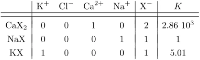
The first example is used as a validation test case. It comes from the documentation of the PhreeqC [27] software, a standard geochemical code, where it is known as “Example 11”. The system is an ion exchange, where a solution of sodium and potassium in equilibrium with an exchanger is injected with calcium-chloride. The reactions involved are as follows
Na++ X− ⇌ NaX K++ X− ⇌ KX 1 2Ca 2+ + X− ⇌ 1 2CaX2
where NaX, KX and CaX2are complexes formed on the surface of the rock matrix, and X represents an exchange
site with charge -1 (see [12] for details on modeling surface reactions). The corresponding Morel tableau is given by For this chemical system, one can see that there are no secondary aqueous species, i.e. we have Q = X (X
K+ Cl− Ca2+ Na+ X− K
CaX2 0 0 1 0 2 2.86 103
NaX 0 0 0 1 1 1
KX 1 0 0 0 1 5.01
(24)
Table 1. Morel tableau for ion exchange example
here is the fictitious concentration of the exchange site, not it’s name).
The quantity that may be determined experimentally is Q and not T . If we start with X and Y (here, we start with X = [2 10−4; 0; 0; 10−3] and Y = [0]), using respectively the Mass Action Law (first line of 12) and the Conservation Law (second line of (12)), we may compute T and W (here, T = [7.51 10−4; 0; 0; 1.55 10−3] and
W = [1.10 10−3]). We can then recompute [Xapp, Yapp] = [T, W ]− ΨC([T, W ]) (since Q = X) and match up
Xappwith X (and Yapp with Y ).
We compare different algorithms, as implemented in the GSL library. For each algorithm, we start with the initial guess [x, y] = max(log10[T, W ],−10) (of course we start with xi =−10 if associated Ti ≤ 0). We run
each algorithm with a relative tolerance of 10−8 and an absolute tolerance of 10−5, and limit the number of iterations to 2000 (considering the algorithm failed if this limit number is reached).
We have compared the classical Newton’s method, without any line search, with two variants of Powell’s hybrid method [28], the difference being in the scaling used for the unknowns, and the fact that the hybrids method uses a finite difference Jacobian. The results are shown in table 2.
Algorithm used XK+ XCl− XCa2+ XNa+ YX− Iters #f #j
Newton 2.00 10−4 0 0 1.00 10−3 0 20 20 20
hybridj 2.00 10−4 0 0 1.00 10−3 0 35 35 3
hybrids 2.00 10−4 0 0 1.00 10−3 0 52 57 0
In table 2, #f and #j are respectively the number of function evaluations and the number of Jacobian evaluation. The Newton algorithm needs the least number of function evaluations, while the hybridj algorithm uses more function evaluations, but only 3 Jacobian evaluations. The finite difference algorithm is not competitive with the methods based on an exact Jacobian. Finally, we note that the hybridj algorithm is more robust, as it converges for several examples when the Newton algorithm fails - see the second test case described in sub-section 3.1.2. In fact, for XCl−, XCa2+ and YX−, one can never have exactly zero (because we solve for the logarithms), but
the result obtained is so much smaller than the relative tolerance that we can consider it is effectively zero. 3.1.2. MoMaS Benchmark (a synthetic example)
The first test case involved only ion exchange. We test now the chemical solver on a more complex system, the "easy test case" of the MoMaS benchmark [6], and see also [23]. Indeed, one should note that “easy” refers to the chemical phenomena taken into account (here no minerals, and no kinetics), as this test case is by no means easy numerically. We recall here the Morel tableau for the chemical system. As can be seen on the tableau, the equilibrium constants span more than 45 orders of magnitude, and some of the stoichiometric coefficients are quite large, making the system very nonlinear. We take for total concentrations T = [0,−2, 0, 2, 1] and either
X1 X2 X3 X4 Y K C1 0 −1 0 0 0 10−12 C2 0 1 1 0 0 1 C3 0 −1 0 1 0 1 C4 0 −4 1 3 0 0.1 C5 0 4 3 1 0 1035 S1 0 3 1 0 1 106 S2 0 −3 0 1 2 0.1 (25)
Table 3. Morel tableau for MoMaS example
W = 1 (test case A) or W = 10 (test case B). We compute the concentrations by using the same algorithms as
in sub-section 3.1.1. The method was validated against a solution obtained by using a Gröbner basis method for solving the polynomial system with a symbolic algebra system.
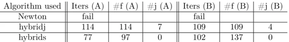
The results are shown in table 4.
Algorithm used Iters (A) #f (A) #j (A) Iters (B) #f (B) #j (B)
Newton fail fail
hybridj 114 114 7 109 109 4
hybrids 77 97 0 102 137 0
Table 4. Comparison of algorithms for the chemical problem - MoMaS benchmark test case
One can see on this table that the “pure” Newton’s method fails, whereas both the hybridj algorithm and the hybrids algorithm converge.
3.1.3. A difficult aqueous system
To see the effects of the initial point choice, we test with another chemical system from [4], or [7]. We recall the Morel tableau of this system (which contains only aqueous species) on table 5.
We take for total concentrations [T ] = [0, 10−3, 10−3], and for both newton and hybridj algorithm we take as initial guess with [x] = [−10, α, β] (in logarithmic form), with α and β varying from −12 to −2, and we limit the maximum number of iterations to 200. On figures 2 and 3, we plot number of iterations needed for convergence with respect to α (horizontal axis) and β (vertical axis).
H+ Al3+ H3L log10K OH− −1 0 0 −14 H2L− −1 0 1 −4.15 HL2− −2 0 1 −12.59 L3− −3 0 1 −23.67 AlHL+ −2 1 1 −4.93 AlL −3 1 1 −9.43 AlL32− −6 1 2 −21.98 AlL63− −9 1 3 −37.69 Al2(OH)2(HL)23− −8 2 3 −22.65 Al2(OH)2(HL)2L3− −9 2 3 −27.81 Al2(OH)2(HL)L4− −10 2 3 −32.87 Al2(OH)2L5− −11 2 3 −39.56 Al4L3+3 −9 4 3 −20.25 Al3(OH)4(H2L)4+ −9 4 3 −12.52 (26)
Table 5. Morel tableau for the gallic acid example
−12 −10 −8 −6 −4 −2 −12 −11 −10 −9 −8 −7 −6 −5 −4 −3 −2 0 20 40 60 80 100 120 140 160 180 200
Figure 2. Convergence of hybridj algorithm
−12 −10 −8 −6 −4 −2 −12 −11 −10 −9 −8 −7 −6 −5 −4 −3 −2 0 20 40 60 80 100 120 140 160 180 200
One can see by comparing figures 2 and 3 that for many choices of the initial guess, Newton’s method is more efficient that the hybridj algorithm. However, we can see a zone (dark red on figure 3) for which the Newton algorithm fails - however the hybridj algorithm still converges.
These tests tend to support the (well known) conclusion that the pure form of Newton’s method is not robust, but that some form of globalization (the hybridj method uses a trust region globalization) makes it much less susceptible to failure when starting far from the solution. This is an especially important issue when the chemical solver is used as a module in a coupled code, as it will be called repeatedly, with little possibility of restarting if it fails.
3.2. Validation of the advection–diffusion part
Results for the flow and transport solvers have already been reported elsewhere [21, 32], so we just give one example to illustrate the performance of these solvers. We use the geometry for the MoMaS benchmark, and compute the transport for species X1, which is an inert tracer, subject only to transport. The domain Ω is made
00000000000000000000000000000000000000000 00000000000000000000000000000000000000000 00000000000000000000000000000000000000000 00000000000000000000000000000000000000000 00000000000000000000000000000000000000000 00000000000000000000000000000000000000000 00000000000000000000000000000000000000000 00000000000000000000000000000000000000000 00000000000000000000000000000000000000000 00000000000000000000000000000000000000000 00000000000000000000000000000000000000000 00000000000000000000000000000000000000000 00000000000000000000000000000000000000000 00000000000000000000000000000000000000000 00000000000000000000000000000000000000000 00000000000000000000000000000000000000000 00000000000000000000000000000000000000000 00000000000000000000000000000000000000000 00000000000000000000000000000000000000000 11111111111111111111111111111111111111111 11111111111111111111111111111111111111111 11111111111111111111111111111111111111111 11111111111111111111111111111111111111111 11111111111111111111111111111111111111111 11111111111111111111111111111111111111111 11111111111111111111111111111111111111111 11111111111111111111111111111111111111111 11111111111111111111111111111111111111111 11111111111111111111111111111111111111111 11111111111111111111111111111111111111111 11111111111111111111111111111111111111111 11111111111111111111111111111111111111111 11111111111111111111111111111111111111111 11111111111111111111111111111111111111111 11111111111111111111111111111111111111111 11111111111111111111111111111111111111111 11111111111111111111111111111111111111111 11111111111111111111111111111111111111111 000 000 000 000 000 000 000 000 000 000 000 000 000 000 000 000 000 000 000 000 000 000 000 000 000 000 000 000 000 000 000 000 000 000 111 111 111 111 111 111 111 111 111 111 111 111 111 111 111 111 111 111 111 111 111 111 111 111 111 111 111 111 111 111 111 111 111 111 B In Out In A
Figure 4. Geometry of the domain Ω for the transport-diffusion part
up of two media : medium A (diagonally dashed) is less permeable and less dispersive than medium B (the barrier, horizontally dashed). The characteristics for both media are given in table 6 (taken from the MoMaS benchmark description [6, 23]). Medium A Medium B Permeability K (LT−1) 10−2 10−5 Porosity ω (-) 0.25 0.5 Dispersivity αL (L) 10−2 6 10−2 Dispersivity αT (L) 10−3 6 10−3
Table 6. Characteristics for the MoMaS benchmark flow and transport example
Note that the contrast in permeabilities for the two media is 1000, so this model presents a fairly stringent test for the ability of the code to handle heterogeneous media.
The boundary conditions for the flow computations are as follows:
• imposed flux on the boundaries labeled “In” ωu1= ωu2= 2.25 10−2LT−1, • imposed head on the boundary labeled “Out” H = 1L,
• no flow on the remaining boundary
and the boundary conditions for transport are
• given concentration on the inflow “In” boundaries Q = 1 • zero diffusive flux on the outflow “Out” boundary,
• zero total flux on the remaining boundary - this condition may be decomposed into two terms :
– no convective flux because we have homogeneous flow velocity condition, – no diffusive flux, giving an homogeneous Neumann condition,
and we take zero initial concentration at time t = 0.
We computed the flow with using the LiFeV environment, and saved it as input for the transport solver.
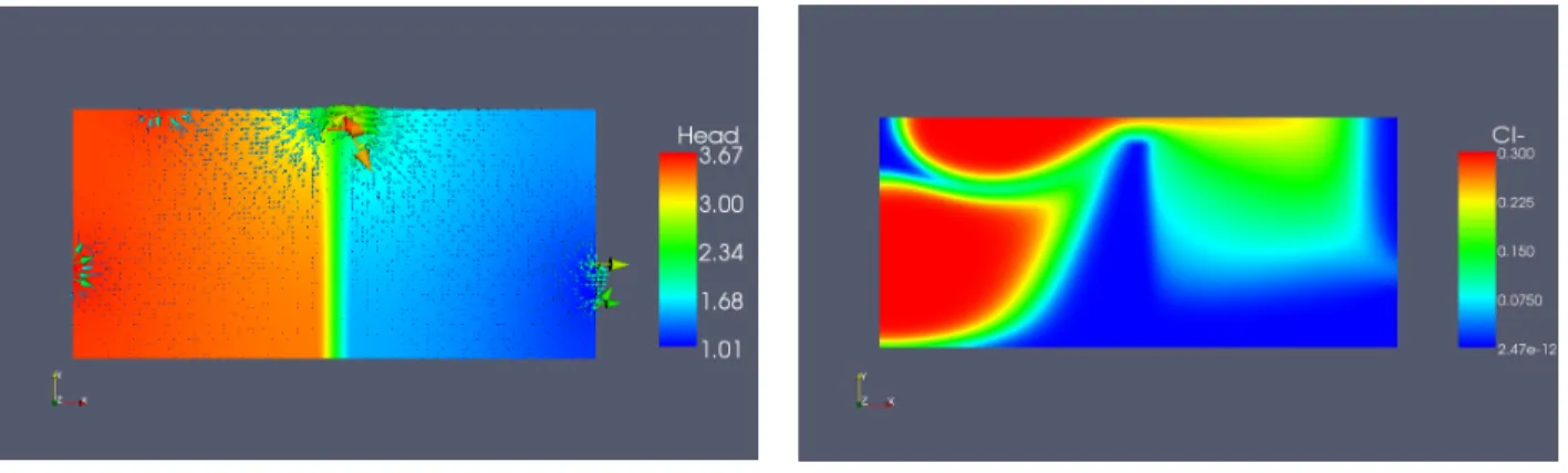
Figure 5. Plot of Darcy velocity and pressure Figure 6. Plot of QCl−
We superimpose on figure 5 the level lines for the pressure on top of the Darcy velocity, and we plot on figure 6 the level lines of the tracer concentration at time t = 25. Qualitatively, we can see that concentration seen on figure 6 follows the Darcy velocity shown on figure 5.
3.3. Coupled system
We now consider the full coupled problem, with the chemical system given by (24), subject now to both transport and chemistry. We consider the simple geometry shown on figure 7:
y axis
x axis
Figure 7. Geometry of the domain Ω for the full test
We assume that the the flow gives rise to a uniform horizontal velocity field given by u = (1, 0)T. We thus do
not need to compute the flow in this case.
With the geometry defined above, we consider two different configurations, depending on the way the CaCl2
is injected: in this first case, the injection occurs along the full left side of the domain, leading to a solution depending only on x (1D configuration). In the second case, the injection occurs only on part of the boundary, giving rise to a truly 2 dimensional solution (2D configuration).
3.3.1. 1D configuration
In this case, the concentration is prescribed along the full left boundary of the computational domain. This corresponds to the ion exchange example from the PhreeqC documentation a;ready mentioned in section 3.1.1. This reference solution will enable us to validate the coupled solution.
For the total aqueous concentrations Qj, we consider :
• Q = [ 0; 1.2 10−3; 6 10−4; 0] on Γ r∪ Γg,
• ∇Q · n = 0 on Γb∪ Γk.
In other words, we start from a porous media which contains K+ and Na+, and we inject on the left side of this media CaCl2, letting the right side free. The idea is, since the Darcy velocity u is parallel to the x-axis, to
get concentrations T , Q and F that only depend on x (assuming that no there is no transverse diffusion, the transport phenomena and boundary conditions are invariant with respect to y).
Figure 8. Plot of different concentrations Qj for time t=20
Figure 8 shows the aqueous concentrations of Ca2+(top-left corner), Na+ (top-right corner), K+(bottom-right corner) at time t = 20, and, since the solutions are constant with respect to y, we also plot the total aqueous concentration of each aqueous species as a function of x (bottom-left corner). Moreover, since each function
Qj is a function of x only, its value at the right boundary only depends on time. We plot the corresponding
“elution curves” on figure 9. This figure can be compared with figure 11, p 241 of the PhreeqC documentation. Interpretation of the results of the figure 9 :
• QCl− (blue line) : since chlorine does not react in our chemical system, it is only subject to transport.
The obtained curve coincides with the well-known solution for a perfect tracer.
• QCa2+ (black line) : if calcium were not affected by chemical reactions, at each time we would have
QCa2+(t) = 0.5QCl−(t) on the right boundary (since the initial data and boundary conditions satisfy this
relation). However, calcium does react, and the reaction is quasi-total (since the equilibrium constant K associated to the reaction Ca2++ 2X− = CaX2 is much larger than 1). This explains why calcium
reaches the right boundary so late.
• QK+ (green line) and QNa+ (red line) : since Ca2+ reacts with X−, we see a disappearance of KX and
NaX. This effect would increase QK+and QNa+. However, we have also transport-diffusion effects, and
since we inject no sodium nor potassium, these effects will decrease QK+ and QNa+. So there are two
Figure 9. Plot of different aqueous concentrations as functions of time
For sodium, transport-diffusion is always more important than chemistry. For potassium,the chemistry effects dominate at first, then the transport takes over.
3.3.2. 2D configuration
In this second case, we only inject the CaCl2 solution on part of the left boundary. For the total aqueous
boundary conditions, we consider the following conditions :
• Q = [ 0; 1.2 10−3; 6 10−4; 0] on Γr,
• ∇Q · n = 0 on ∂Ω \ Γr.
The object of this test is to show truly 2D effects, and not only a 1D solution computed on a 2D grid. We show on figure 10 the aqueous concentration of Cl− (top-left corner), Ca2+(top-right corner), K+(bottom-left corner) and Na+ (bottom-right corner) at time t = 35. We find results that can be explained according to the theory. In particular, chlorine is still a perfect tracer, and an analytical solution has been computed by Feike and Dane [13], and our results show a good agreement with this solution. The other concentrations can be explained from the chemical point of view as in the previous section.
Acknowledgments
Part of the work reported in this paper took place during the Cemracs summer school in August 2008. The authors thank the organizers of the Cemracs for making possible a very productive (and pleasant) session.
References
[1] L. Amir and M. Kern. Newton - Krylov methods for coupling transport with chemistry in heterogeneous porous media.
Computational Geosciences, 2009. submitted.
[2] J. Bear and A. Verruijt. Modeling Groundwater Flow and Pollution. Theory And Applications Of Transport In Porous Media. Kluwer Academic Publishers Group, 1987.
[3] J. Blom and J. Verwer. A comparison of integration methods for atmospheric transport-chemistry problems. J. Comp. Appl.
Math., 126:381–396, 2000.
[4] P. Brassard and P. Bodurtha. A feasible set for chemical speciation problems. Computers & Geosciences, 26(3):277 – 291, 2000.
[5] F. Brezzi and M. Fortin. Mixed and Hybrid Finite Element Methods. Springer Series in Computational Mathematics. Springer, Berlin, 1991.
[6] J. Carrayrou, M. Kern, and P. Knabner. presentation of the MoMaS reactive transport benchmark. Computational Geosciences, 2009. to appear, special issue on MoMaS Reactive Transport Benchmark.
[7] J. Carrayrou, R. Mosé, and P. Behra. New Efficient Algorithm for Solving Thermodynamic Chemistry. AIChE Journal, 48:894–904, 2002.
Figure 10. Instants snapshots of the aqueous concentration of Cl− (top-left corner), Ca2+ (top-right corner), K+ (bottom-left corner) and Na+ (bottom-right corner)
[8] C. de Dieuleveult and J. Erhel. A numerical model for coupling chemistry and transport. In International Conference on
SCIentific Computation And Differential Equations, SciCADE 2007, 2007.
[9] C. de Dieuleveult, J. Erhel, and M. Kern. A global strategy for solving reactive transport equations. Journal of Computational
Physics, In Press, Corrected Proof:–, 2009.
[10] G. de Marsily. Hydrogéologie quantitative. Masson, 1981.
[11] L. J. Durlofsky. Accuracy of mixed and control volume finite element approximations to Darcy velocity and related quantities.
Water Resour. Res.,, 30(4):965–973, 1994.
[12] D. Dzombak and F. Morel. Surface complexation modeling–Hydrous ferric oxide. John Wiley, 1993.
[13] L. Feike and J. H. Dane. Analytical solution of the one dimensional advection equation and two- and three- dimensional dispersion equation. Water Resources Res., 26:1475–1482, 1990.
[14] M. Galassi, J. Davies, J. Theiler, B. Gough, G. Jungman, M. Booth, and F. Rossi. GNU Scientific Library Reference Manual
- Revised Second Edition (v1.8). Network Theory Ltd, 2006.
[15] G. E. Hammond, A. Valocchi, and P. Lichtner. Application of Jacobian-free Newton–Krylov with physics-based preconditioning to biogeochemical transport. Advances in Water Resources, 28:359–376, 2005.
[16] C. J., R. Mosé, and P. Behra. Efficiency of operator splitting procedures for solving reactive transport equation. J. Contam.
Hydrol., 68:239–268, 2004.
[17] S. Kraütle. General multi-species reactive transport problems in porous media: Efficient numerical approaches and existence of
global solutions. Habilitation thesis, University of Erlangen, 2008. http://www1.am.uni-erlangen.de/~kraeutle/habil.pdf.
[18] S. Kraütle and P. Knabner. A new numerical reduction scheme for fully coupled multicomponent transport-reaction problems in porous media. Water Resources Research, 41(W09414), 2005.
[19] S. Kraütle and P. Knabner. A reduction scheme for coupled multicomponent transport-reaction problems in porous media: Generalization to problems with heterogeneous equilibrium reactions. Water Resources Research, 43(W03429), 2007. [20] J. D. Logan. Transport modelling in hydrogeochemical systems. Springer, 2001.
[21] E. Marchand. Analyse de sensibilité déterministe pour la simulation numérique du transfert de contaminants. thèse de doctorat, Université Paris IX Dauphine, 2007.
[22] A. Mazzia, L. Bergamaschi, and M. Putti. A time-splitting technique for the advection-dispersion equation in groundwater. J.
Comput. Phys., 157(1):181–198, 2000.
[23] G. MoMaS. Exercices de qualification numérique de codes. http://www.gdrmomas.org/ex_qualifications.html, 2004. [24] P. Montarnal, A. Dimier, E. Deville, E. Adam, J. Gaombalet, A. Bengaouer, L. Loth, and C. Chavant. Coupling
on Computational Methods for Coupled Problems in Science and Engineering, Barcelona, 2005. CIMNE. available as
http://hal.archives-ouvertes.fr/hal-00116195/fr/.
[25] F. Morel and J. G. Hering. Principes and Applications of Aquatic Chemistry. Wiley, 1993.
[26] R. Mosé, P. Ackerer, P. Siegel, and G. Chavent. Application of the mixed hybrid finite element approximation in a groundwater flow model : Luxury or necessity. Water Ressources Res., 30:3001–3012, 1994.
[27] D. L. Parkhurst and C. Appelo. User’s guide to PHREEQC (version 2)- A computer program for speciation, batch-reaction, one-dimensional transport, and inverse geochemical calculations. Technical Report 99-4259, USGS, 1999.
[28] M. J. D. Powell. A hybrid method for nonlinear equations. In P.Rabinowitz, editor, Numerical Methods for Nonlinear Algebraic
Equations, pages 87–114. Gordon and Breach, 1970.
[29] J. E. Roberts and J.-M. Thomas. Mixed and hybrid methods. In P. G. Ciarlet and J.-L. Lions, editors, Handbook of Numerical
Analysis, Finite Element Methods, volume II, pages 523–639. North-Holland, 1991.
[30] J. Rubin. Transport of reacting solutes in porous media: relation between mathematical nature of problem formulation and chemical nature of reaction. Water Resources Res., 19:1231–1252, 1983.
[31] M. Saaltink, J. Carrera, and C. Ayora. On the behavior of approaches to simulate reactive transport. Journal of Contaminant
Hydrology, 48:213–235, 2001.
[32] A. Sboui. Quelques méthodes numériques robustes pour l’écoulement et le transport en milieu poreux. thèse de doctorat, Université Paris IX Dauphine, 2007.
[33] P. Siegel, R. Mosé, P. Ackerer, and J. Jaffré. Solution of the advection-dispersion equation using a combination of discontinuous and mixed finite elements. Journal for Numerical Methods in fluids, 24:595–613, 1997.
[34] C. Steefel, D. DePaolo, and P. Lichtner. Reactive transport modeling: An essential tool and a new research approach for the Earth sciences. Earth and Planetary Science Letters, 240:539–558, 2005.
[35] A. Valocchi. Validity of the local equilibrium assumption for modeling sorbing solute transport through homogeneous soils.
Water Resources Res., pages 808–820, 1985.
[36] J. van der Lee. CHESS, another speciation and surface complexation computer code. Technical Report LHM/RD/93/39, CIG École des Mines de Paris, Fontainebleau, 1993.
[37] G. T. Yeh and V. S. Tripathi. A critical evaluation of recent developments in hydrogeochemical transport models of reactive multichemical components. Water Res. Res., 25:93–108, 1989.