HAL Id: inria-00530758
https://hal.inria.fr/inria-00530758v2
Submitted on 4 Mar 2011
HAL is a multi-disciplinary open access
archive for the deposit and dissemination of sci-entific research documents, whether they are pub-lished or not. The documents may come from teaching and research institutions in France or
L’archive ouverte pluridisciplinaire HAL, est destinée au dépôt et à la diffusion de documents scientifiques de niveau recherche, publiés ou non, émanant des établissements d’enseignement et de recherche français ou étrangers, des laboratoires
Parametrization of computational domain in
isogeometric analysis: methods and comparison
Gang Xu, Bernard Mourrain, Régis Duvigneau, André Galligo
To cite this version:
Gang Xu, Bernard Mourrain, Régis Duvigneau, André Galligo. Parametrization of computational domain in isogeometric analysis: methods and comparison. Computer Methods in Applied Mechan-ics and Engineering, Elsevier, 2011, 200 (23-24), pp.2021-2031. �10.1016/j.cma.2011.03.005�. �inria-00530758v2�
Parametrization of computational domain in isogeometric analysis:
methods and comparison
Gang Xua,d, Bernard Mourraina, R´egis Duvigneaub, Andr´e Galligoc
a
Galaad, INRIA Sophia-Antipolis, 2004 Route des Lucioles, 06902 Cedex, France
b
OPALE, INRIA Sophia-Antipolis, 2004 Route des Lucioles, 06902 Cedex, France
c
University of Nice Sophia-Antipolis, 06108 Nice Cedex 02, France
d
College of Computer, Hangzhou Dianzi University, Hangzhou 310018, P.R.China
Abstract
Parameterization of computational domain plays an important role in isogeometric analysis as mesh generation in finite element analysis. In this paper, we investigate this problem in the 2D case, i.e, how to parametrize the computational domains by planar B-spline surface from the given CAD objects (four boundary planar B-spline curves). Firstly, two kinds of sufficient conditions for injective B-spline parameterization are derived with respect to the control points. Then we show how to find good parameterization of computational domain by solving a constraint optimization problem, in which the constraint condition is the injectivity sufficient conditions of planar B-spline parametrization, and the optimization term is the minimization of quadratic energy functions related to the first and second derivatives of planar B-spline parameterization. By using this method, the resulted parameterization has no self-intersections, and the isoparametric net has good uniformity and orthogonality. After introducing a posteriori error estimation for isogeometric analysis, we propose r-refinement method to optimize the parameterization by repositioning the inner control points such that the estimated error is minimized. Several examples are tested on isogeometric heat conduction problem to show the effectiveness of the proposed methods and the impact of the parameterization on the quality of the approximation solution. Comparison examples with known exact solutions are also presented.
Keywords: isogeometric analysis; injectivity of B-spline parameterization; constraint
optimization method; a posteriori error estimation; r-refinement
Email addresses: [email protected], [email protected](Gang Xu), [email protected] (Bernard Mourrain), [email protected] (R´egis Duvigneau), [email protected] (Andr´e Galligo)
1. Introduction
The isogeometric analysis (IGA for short) approach originally proposed by Hughes et al. in [25] can be employed to overcome the gap between CAD and finite element analysis (FEA for short) by using the same geometric representation based on NURBS for all design and analysis tasks. This framework allows to compute the analysis results on the exact CAD geometry rather than a discretized mesh geometry, to obtain a more accurate solution by high-order approximation, to reduce spurious numerical sources of noise that deteriorate convergence, and to avoid data exchanges between the design and analysis phases. Furthermore, NURBS representation allows to perform refinement operations to improve the simulation result by knot insertion and degree elevation.
Mesh generation, which generates a discrete mesh of a computational domain from a given CAD object, is a key and the most time-consuming step in FEA. It consumes about 80% of the overall design and analysis process [7] in automotive, aerospace and ship industry. Parametrization of computational domain in IGA, which corresponds to the mesh generation in FEA, also has some impact on analysis result and efficiency. In particular, arbitrary refinements can be performed on the computational mesh in FEA, but in IGA if we compute with tensor product B-splines, we can only perform refinement operations in u direction and v direction by knot insertion or degree elevation. Hence, parameterization of computational domain is also being important for IGA.
In IGA, the parameterization of a computational domain is determined by control points, knot vectors and the degrees of B-spline objects. For IGA problem of two dimensions, the knot vectors and the degree of the computational domain are determined by the given boundary curves. That is, given boundary curves, the quality of parameterization of computational domain is determined by the positions of inner control points. Hence, finding a good placement of the inner control points inside the computational domain, is a key issue. A basic requirement of the resulting parameterization for IGA is that it doesn’t have self-intersections, so that it is an injective map from the parametrization domain to the computational domain. In order to get more accurate simulation results, the isoparametric net in the computational domain should be as uniform as possible and have orthogonal isoparametric curves [8]. In this paper, we investigate this problem in 2D case, i.e, how to construct the computational domains (planar B-spline surface) from the given CAD objects (four boundary planar spline curves). Firstly, Two kinds of sufficient conditions for injective
B-spline parameterization are derived with respect to the control points. Then the parameterization of the computational domain is considered as a constraint optimization problem, in which the constraint condition is the injectivity sufficient conditions of planar B-spline parameterization, and the optimization term is the minimization of quadratic energy functions related to the first and second derivatives of the computational domain (B-spline surface). By using this method, the resulted parameterization has no self-intersection, and the isoparametric net has good uniformity and orthogonality.
In IGA, there are three kinds of methods to improve the simulation results by increasing degree of freedom: h-refinement by knot insertion, p-refinement by order elevation, and k-refinement com-bining order elevation and knot insertion [13,19,27]. The common feature of above three methods is that the degree of freedom (control points in IGA) is increased while keeping the geometry of computational domain. In FEA, r-refinement is a remesh operation on computational domain to minimize the cost function while keeping the number of elements as a constant [31, 10]. In this paper, as the second method for optimizing the parametrization of computational domain, based on a residual-based a posteriori error estimation, an isogeometric r-refinement method is proposed to optimize the parameterization of the computational domain by minimizing the estimated er-ror. It is a generalization of the optimal parameterization method proposed in [34], in which only the problem with a known exact solution is investigated. Several examples have been tested on isogeometric heat conduction problems to show the effectiveness of the proposed methods.
The remainder of the paper is organized as follows. Section2reviews the related work in IGA. Section3presents two kinds of sufficient conditions for injectivity of planar B-spline parameteriza-tion. Section4describes the constraint optimization method for parameterization of computational domain. r-refinement method and a posteriori error estimation is presented in5. Some examples and comparisons based on the isogeometric heat conduction problem are presented in Section 6. Finally, we conclude this paper and outline future works in Section 7.
2. Related work
In this section, some related works in IGA and parameterization of computational domains will be reviewed.
of CAD and FEA. Since then, many researchers in the fields of computational mechanical and geometric computation were involved in this topic. The current work on isogeometric analysis can be classified into three categories: (1) application of IGA to various simulation and analy-sis problems [3, 6, 5, 14, 18, 24, 26, 35]; (2) application of various modeling tools in geometric computation to IGA [7,16,29,9]; (3) accuracy and efficiency improvement of IGA framework by reparameterization and refinement operations [1,4,12,13, 19,27,30,34].
The topic of this paper belongs to the third field. As far as we know, there are few works on the parametrizations of computational domains for IGA. T. Martin et al. [30] proposed a method to fit a genus-0 triangular mesh by B-spline volume parameterization, based on discrete volumetric harmonic functions; this can be used to build computational domains for 3D IGA problems. A variational approach for constructing NURBS parameterization of swept volumes is proposed by M. Aigner et al [1]. Many free-form shapes in CAD systems, such as blades of turbines and propellers, are covered by this kind of volumes. E. Cohen et.al. [12] proposed the concept of analysis-aware modeling, in which the parameters of CAD models should be selected to facilitate isogeometric analysis. They also demonstrated the influence of parameterization of computational domains by several examples. Approximate implicitization technique is used for parametrization of computational domain in [33]. In [34], a method for generating optimal analysis-aware parameterization of computational domain is proposed based on shape optimization method. However, it only works for problems with exact solutions. In this paper, we propose a general method to generate analysis-suitable parameterization of computational domain in IGA.
3. Sufficient conditions for injective B-spline parameterization
The concept of isogeometric analysis consists in representing the physical quantities Φ ∈ Rp on the geometry Ω using the same type of mathematical representation as for the geometry Ω. In other words, given a point x = σ(ξ, η) ∈ Ω with (ξ, η) ∈ P, we associate to it the physical quantity Φ(ξ, η) where Φ(ξ, η) is a B-spline function with knots in P and control points in Rp. This means
that the map x ∈ Ω 7→ Φ ∈ Rp is defined implicitly as x 7→ Φ ◦ σ−1(x).
Consequently, the framework of isogeometry is thus valid when the parameterization σ of the geometry is injective (or bijective on its image). We will consider this issue in the context of finding a “good” parameterization of a domain when its boundary is given. In [28], a general sufficient
condition is proposed for injective parameterization.
Proposition 3.1. Suppose that σ is a C1 parameterization from a compact domain P ⊂ Rn with
a connected boundary to a geometry Ω ⊂ Rn. If σ is injective on the boundary ∂P of P and its
Jacobian Jσ does not vanish on P, then σ is injective.
For a parameterization σ from P : [a, b] × [c, d] to Ω ⊂ R2, we define the boundary curves as the image of {a} × [c, d], {b} × [c, d], [a, b] × {c}, [a, b] × {d} by σ. We say that σ defines a regular
boundary if these curves do not intersect pairwise, except at their end points and if they have no
self-intersection points.
As a consequence of the previous proposition, we get the following injectivity test for standard B-spline tensor product parameterization of a planar domain.
Proposition 3.2. Let σ be a C1 parameterization from [a, b] × [c, d] to Ω ⊂ R2 which defines a regular boundary. If its Jacobian Jσ does not vanish on [a, b] × [c, d], then σ is injective.
We consider first the case of a planar parameterization σ : (ξ, η) ∈ P := [a, b] × [c, d] 7→ σ(ξ, η) := X 0≤i≤n 0≤j≤m ci,jNip(ξ)N q j(η),
where ci,j ∈ R2 are the control points, Nip(ξ) and Njq(η) are B-spline basis functions of degree p
and q for a given knot vector on [a, b] and [c, d] .
The derivative of σ(ξ, η) with respect to ξ can be expressed in terms of the differences ∆1i,j := (∆1,xi,j, ∆1,yi,j) = ci+1,j− ci,j:
∂ξσ(ξ, η) :=
X
0≤i≤n−1 0≤j≤m
ω1i,j∆1i,jNip−1(ξ)Njq(η), (1)
where Nip−1(ξ) is the B-spline basis function with one degree less in u, ω1
i,j is a positive factor.
Similarly, the derivative of σ(ξ, η) with respect to η can be expressed in terms of the differences ∆2
i,j:= (∆ 2,x
i,j, ∆
2,y
i,j) = ci,j+1− ci,j:
∂ησ(ξ, η) := X 0≤i≤n 0≤j≤m−1 ω2i,j∆2i,jN p i(ξ)N q−1 j (η), (2)
3.1. Non-linear sufficient condition based on Jacobian computation
From Proposition3.2, if the Jacobian determinant J (σ(ξ, η)) of planar B-spline parameteriza-tion satisfies J (σ(ξ, η)) > 0, σ(ξ, η) has no self-intersecparameteriza-tions.
From (1), (2) and the product properties of B-splines [32] , the Jacobian determinant J (σ(ξ, η)) of B-spline surface can be computed as follows:
J(σ(ξ, η)) = σx ξ σηx σyξ σyη = σξxσyη − σξxσηy = X 0≤i≤n−1 0≤j≤m X 0≤i′≤n 0≤j′≤m−1 Nip−1(ξ)Njq(η) Nip′(ξ)N q−1 j′ (η) ω1i,jωi2′,j′ ∆1,xi,j ∆2,xi,j ∆1,yi′,j′ ∆ 2,y i′,j′ (3) = 2n−1 X i=0 2m−1 X j=0 GijNi2p−1(ξ)N 2q−1 i (η) (4)
Hence, the Jacobian of planar B-spline parameterization can be represented in the form of B-spline surface with higher degrees. From the convex hull property of B-spline surface [20], we have the following theorem.
Theorem 3.3. If Gij > 0 in (4), then J(σ(ξ, η)) > 0, that is, σ(ξ, η) has no self-intersections.
This is a non-linear sufficient condition with respect to the inner control points. In Section4, we will employ it as constraint term in the constraint optimization method for general case.
Notice that if the coefficients ω1i,jω2i′,j′
∆1,xi,j ∆2,xi,j ∆1,yi′,j′ ∆ 2,y i′,j′
in the expansion (3), we also obtain a sufficient condition for J (σ(ξ, η)) 6= 0. But the conditions Gij > 0 are weaker than these conditions,
since the coefficient matrix which expresses the elements Nip−1(ξ)Njq(η) Nip′(ξ)N
q−1
j′ (η) in terms of
the elements (Ni2p−1(ξ)Ni2q−1(η))1≤i≤2n−1,1≤j≤2m−1, has positive coefficients.
3.2. Linear sufficient condition using injectivity cones
In this subsection, we propose a linear sufficient condition for injectivity of a B-spline param-eterization.
We denote by C1(c) the convex cone of R2 generated by the half rays R+· ∆1i,j. We denote by
C2(c) the convex cone of R2 generated by the half rays R+· ∆2i,j. If this cone is generated by two
(a) (b)
Fig. 1. Injectivity test using cones: (a) transverse case; (b) non-transverse case.
We say that two cones C1, C2 are transverse if R · C1 and R · C2 intersect only at {0}.
In [34], a sufficient and easy-to-check condition is proposed to ensure the local injectivity of σ. Proposition 3.4. Let σ be a B-spline parametrisation, which is at least C1 from P := [a, b] × [c, d] to Ω ⊂ R2 given by the control points c. If the boundary curves do not intersect and have no
self-intersection point and the cones C1(c), C2(c) are transverse, then σ is injective on P.
Fig. 1 shows two examples of the injectivity testing method.
This linear condition can be used to devise an algorithm which constructs an injective param-eterization from given boundary control points. Given four planar boundary curves described by the controls points ci,0, ci,m, c0,j, cn,j, with 0 ≤ i ≤ n, 0 ≤ j ≤ m, we define the boundary cone
C0
1(c) (resp. C20(c)) as the cone generated by the vectors ∆1i,0(c), ∆1i,m(c) for 0 ≤ i ≤ n − 1 (resp.
∆20,j(c), ∆2m,j(c) for 0 ≤ j ≤ m − 1). We assume that these two boundary cones C10(c), C20(c) are transverse and R · C10(c) is the boundary cone defined by F1+(C10(c)) ≤ 0, F1−(C10(c)) ≤ 0, where F1+
and F1− are the linear equations defining the boundary of R · C10(c). We defined similarly F2+, F2−
for C20(c).
In [34], the following linear sufficient condition for injective parameterization are proposed,
F2+(ci+1,j− ci,j) + F1−(ci+1,j− ci,j) ≤ 0, F2−(ci+1,j− ci,j) + F1+(ci+1,j − ci,j) ≤ 0,
F2+(ci,j+1− ci,j) + F1−(ci,j+1− ci,j) ≤ 0, F2−(ci,j+1− ci,j) + F1+(ci,j+1− ci,j) ≤ 0,
(5) where 0 < i < n, 0 ≤ j < m.
This set of conditions provides linear constraints for the injectivity of planar B-spline pa-rameterization. In the following section, we will employ it as constraint term in the quadratic programming method for the case when the boundary cones are transverse.
4. Constraint optimization method for parametrization of computational domains In this section, we aim at finding injective parameterization of the computational domain with a uniform and orthogonal isoparametric net.
4.1. Initial construction of inner control points
In order to solve this constraint optimization problem, an initial construction of inner control points is required. We rely on the discrete Coons method presented in [21] to generate inner control points as initial value from boundary control points. See Fig. 4.1(a) for an example.
Given the boundary control points c0,j, cn,j, ci,0, ci,m, i = 0, . . . , n, j = 0, . . . , m, the inner
control points ci,j (i = 1, . . . , n − 1, j = 1, . . . , m − 1) can be constructed by the discrete Coons
method as follows: ci,j = (1 − i n)c0,j+ i ncn,j + (1 − j m)ci,0+ j mci,m −[1 − i n i n] c0,0 c0,m cn,0 cn,m 1 −mj j m
Remark 4.1. Since the sum of the coefficients equals 1, the resulting inner control points lie in the convex hull of the boundary control points.
Remark 4.2. For some given boundary curves, this construction may cause some self-intersections, and lead to an improper parameterization for IGA. See Fig. 4.1 (b) for such an example.
Remark 4.3. The discrete Coons method can be generalized to trivariate case, which can be used for generation of parametric B-spline volumes. See Appendix for details.
4.2. Non-linear constraint optimization method for uniform and orthogonal grid
An internal energy function of the computational domain will be used as an optimization term in a constraint optimization method to construct a computational domain with an uniform and orthogonal isoparametric net.
A parametric surface σ(ξ, η) has orthogonal isoparametric curves if and only if it satifies the following condition
(a) (b)
Fig. 2. Examples of Coons surface: (a) example without self-intersection ; (b) example with self-intersections.
Green control points are inner control points generated by discrete Coons method.
Hence by minimizing the following energy functions, one can achieve isoparametric net with or-thogonal isoparametric curves,
Z
(σξ· ση)2dξdη. (7)
As |σξ· ση| ≤ kσξk
2+kσηk2
2 , in order to get quadratic energy functions with respect to interior control
points, we can minimize the following energy function Z Z
k σξ k2 + k ση k2 dξdη. (8)
The uniformity of the iso-parametric net on the B-spline surface is related to the following quantity: Z Z
(k σξξ k2+ k σηη k2 +2 k σξη k2)dξdη. (9)
In [11], the above two energy functions (8) and (9) are called stretch energy and bend energy respectively, which depend only on intrinsic property of the surface. In summary, combining (8) and (9), we use the following optimization term as objective function,
min Z Z
(k σξξk2 + k σηη k2 +2 k σξη k2) + ω(k σξk2 + k ση k2)dξdη
where ω is a positive constant.
This leads to the following constraint optimization algorithm based on the non-linear sufficient condition in subsection3.1:
Input: four coplanar boundary B-spline curves
(a) (b) (c)
Fig. 3. Example of non-linear constraint optimization method: (a) given boundary B-spline curves; (b) initial
Coons surface; (c) final optimization result;
• Construct the initial inner control points as in subsection 4.1;
• Construct the constraints condition (5) from boundary B-spline curves as in Section3; • Solve the following constraint optimization problem by using SQP method
min Z Z
(k σξξ k2 + k σηη k2 +2 k σξη k2) + ω(k σξk2+ k ση k2)dξdη
s.t. Gij > 0
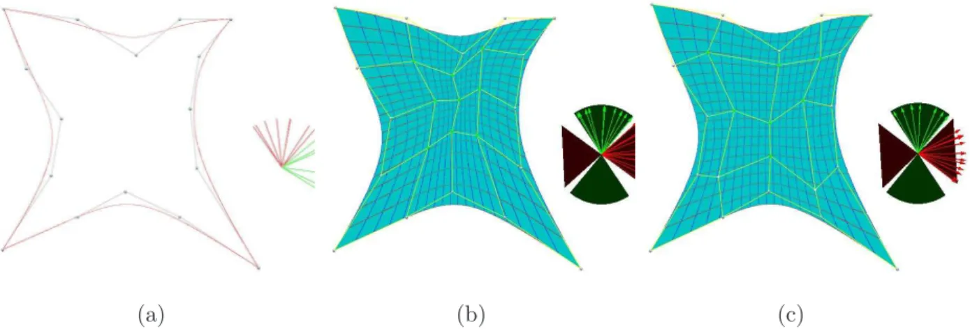
• Generate the corresponding planar B-spline surface σ(ξ, η) as computational domain. As this method is a non-linear constraint optimization algorithm, it can be used also for more general cases, including the case where the boundary injectivity cones are non-transverse. An example of the application of this method is illustrated in Fig. 3. Fig. 3 (a) presents the given boundary curves. Fig. 3 (b) shows the initial Coons surface with self-intersections. The optimization result by non-linear constraint optimization method is shown in Fig. 3 (c). The optimization result avoids self-intersection and gives more uniform iso-parametric grid.
4.3. Quadratic programming method for parametrization of computational domain
If the boundary injectivity cones are transverse, we can propose a quadratic programming method for parameterization of computational domain as follows:
Input: four coplanar boundary B-spline curves
(a) (b) (c)
Fig. 4. Example of quadratic programming method: (a) given boundary B-spline curves and boundary cones; (b)
initial Coons surface; (c) final optimization result.
• Construct the initial inner control points as in subsection 4.1;
• Construct the constraints condition (5) from boundary B-spline curves as in Section3; • Solve the following constraint optimization problem by using a quadratic programming
method, min Z Z (k σξξ k2+ k σηη k2 +2 k σξη k2) + ω(k σξk2 + k ση k2)dξdη s.t.
F2+(ci+1,j− ci,j) + F1−(ci+1,j− ci,j) ≤ 0, F2−(ci+1,j− ci,j) + F1+(ci+1,j− ci,j) ≤ 0,
F2+(ci,j+1− ci,j) + F1−(ci,j+1− ci,j) ≤ 0, F2−(ci,j+1− ci,j) + F1+(ci,j+1− ci,j) ≤ 0,
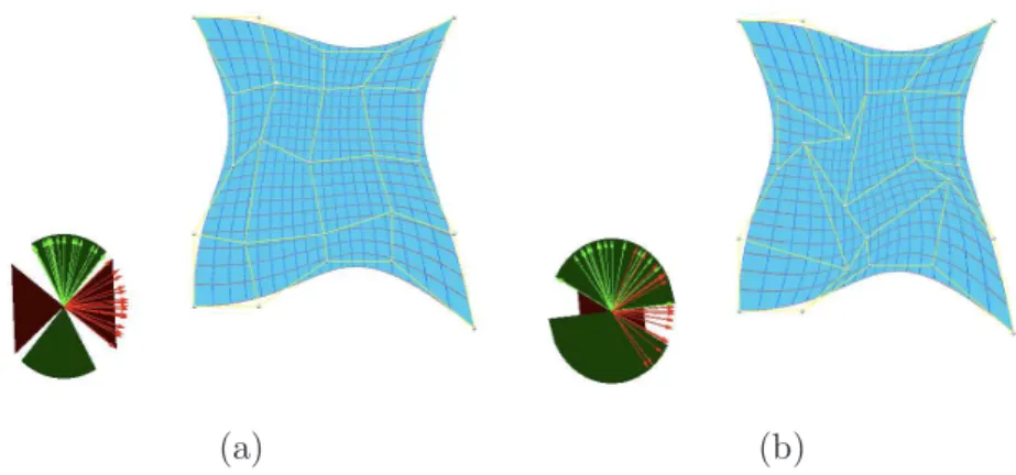
• Generate the corresponding planar B-spline surface σ(ξ, η) as computational domain. Fig. 4 illustrates an example. The given boundary B-spline curves and boundary injectivity cones are shown in Fig. 4(a). The initial Coons surfaces is shown in Fig. 4 (b), and we can obtain a better parameterization as illustrated in Fig. 4 (c) by quadratic programming method. Quantitative data of constraint optimization method for parameterization of computational domain in Fig.3 and Fig.4 is summarized in Table.1.
Remark 4.4. This second method is more efficient because the constraint conditions are linear and easy to compute.
Table 1: Quantitative data for parameterization of computational domain in Fig.3 and Fig.4. # deg.: degree of B-spline parameterization; # con.: number of control points; # iter.: number of optimization iterations.
Example # Deg. # Con. #Iter.
Fig.3 3 45 5
Fig.4 3 25 4
5. r-refinement in isogeometric analysis
In this section, we will propose the isogeometric version of r-refinement for problems with unknown exact solutions, which is a generalization of the method presented in [34]. We firstly propose a residual-based a posteriori error estimation for specified model problem, then present r-refinement method to optimize the placement of inner control points.
5.1. Model problem
For ease of presentation, we consider the two dimensional second order elliptic PDE with homogeneous Dirichlet boundary condition as an illustrative model problem :
−∆U (x) = f (x) in Ω U (x) = 0 on ∂Ω
(10)
where x are the Cartesian coordinates, Ω is a Lipschitz domain with boundary ∂Ω, f (x) ∈ L2(Ω) : Ω 7→ R is a given source term, and U(x) : Ω 7→ R is the unknown solution.
The weak form of (10) is given by: find U (x) ∈ H01(Ω), such that
B(U, V ) = (f, V ), ∀ V ∈ H01(Ω) (11) where B(U, V ) = Z Ω ∇U (x) ∇V (x) dx, (f, V ) = Z Ω f (x) V (x) dx, ∀ U, V ∈ H01(Ω) The energy norm and L2(Ω) norm of U ∈ H1
0(Ω) are defined by kU kE(Ω) = pB(U, U) and
5.2. Residual-based a posteriori error estimate
The isogeometric solution Uh ∈ U(σ) of the problem (10) satisfies
B(Uh, Vh) = (f, Vh), ∀Vh ∈ U(σ), (12)
where U(σ) ⊂ H01(Ω) is a suitable subspace of H01(Ω) based on a parametrization σ of Ω.
We assume that U is the exact solution. Let eh = U − Uh be the error of the isogeometric
approximation Uh. From (11) and (12) , we have for arbitrary V ∈ H01(Ω)
B(eh, V ) = B(U, V ) − B(Uh, V ) = (f, V ) − B(Uh, V )
= Z Ω f (x) V (x) dx − Z Ω ∇Uh(x) ∇V (x) dx = X K∈σ { Z K f (x) V (x) dx − Z K ∇Uh(x) ∇V (x) dx} (13)
where K is the sub-patch in the B-spline parameterization σ(ξ, η) of Ω with respect to the knot elements in the parametric domain P.
After integrating by parts and rearranging terms, we obtain B(eh, V ) = X K∈σ Z K RK(x)V (x) dx + X γ∈Zh Z γ JγV (x) dx (14)
where RK is the interior sub-patch residual
RK(x) = f (x) + ∆Uh(x) in K, (15)
and Jγ is the jump of the gradient across the curved edge γ ∈ Zh between sub-patches,
Jγ = n· ∇Uh+ n ′ · ∇Uh′, if γ /∈ ∂Ω 0, if γ ∈ ∂Ω (16)
where on curved edges between interior patches, γ /∈ ∂Ω, the curved edge γ separates sub-patches K and K′.
Notice that Jγ = 0 in (16) due to the continuity of ∇Uh in isogeometric analysis. Hence, we
have B(eh, V ) = X K∈σ Z K RK(x)V (x) dx (17)
For given V ∈ H01(Ω), denote by IhV the interpolation of V on U(σ). Then the orthogonality
property implies B(eh, IhV ) = 0, and by (17), we obtain
B(eh, V ) = X K∈σ Z K RK(x)(V (x) − IhV (x)) dx, (18)
From Cauchy-Schwartz inequality, B(eh, V ) ≤ X K∈σ Z K kRK(x)kL2(K)kV (x) − IhV (x)kL2(K)dx, (19)
Letting V = eh, from the properties of bilinear form B(·, ·) and the approximation theory [2],
we can obtain the residual-based a posteriori error estimate in isogeometric analysis: kehk2E(Ω)≤ C
X
K∈σ
h2KkRKk2L2(K) (20)
where C is a constant and hK is the diameter of patch K ∈ σ.
5.3. Optimization method
In the proposed approach, we minimize the estimated error from the IGA solution, by moving inner control points of the computational domain. Therefore, we consider as optimization variables the coordinates of the inner control points and as cost function the error of the IGA solution. The optimization algorithm used for this study is a classical steepest-descent method in conjunction with a back-tracking line-search. For this exercise, the gradient of the cost function is approximated using a centered finite-differencing scheme.
Each iteration k of the optimization algorithm can be summarized as follows, starting from a point xk in the variable space:
1. Evaluation of perturbed points xk+ ǫek
2. Estimation of the gradient ∇f (xk) by finite-difference
3. Define search direction dk= −∇f (xk)
4. Line search : find ρ such as f (xk+ ρdk) < f (xk)
5.4. Overview of r-refinement method in IGA
Based on the proposed error estimation, the procedure of r-refinement for model problem (10) can be described as follows,
Input: initial planar B-spline parameterization σ(ξ, η) of computational domain Ω Output: final planar B-spline parametrization σf inal(ξ, η) of Ω after r-refinement
• compute the isogeometric solution Uh(x) = Uh(x(ξ, η), y(ξ, η)) = T (ξ, η) of model problem
(10) over given parameterization σ(ξ, η) of computational domain Ω ; • reposition inner control points by minimizingP
K∈σh2Kkf (x)+ ∆Uh(x)k2L2(K) with
optimiza-tion method in Subsecoptimiza-tion5.3;
• output final placement of inner control points and corresponding planar B-spline parameter-ization.
In the second step, the problem of determining the position of the interior control points is expressed as an optimal control problem. Thus, we propose to locate the interior control points in order to minimise a cost functional that approximates the norm of the error. The cost func-tional depends non-linearly on the control points location, through the computation of the PDE solution and the approximated error. The minimization is then achieved using a classical steepest descent method, associated with a back-tracking line-search that allows to fulfill Armijo-Goldstein convergence criteria [23].
Fig. 5 shows an example from [34], which has exact solution for problem (10) over the given computational domain in Fig. 5(a). Initial error color map computed as difference between exact solution and IGA solution is shown in Fig. 5 (b), final computational domain by r-refinement method based on the estimated error is illustrated in Fig. 5 (c), Fig. 5 (d) shows the error color map obtained from computational domain in Fig. 5 (c); the final computational domain in [34] obtained by minimizing the exact error is shown Fig. 5 (e), Fig. 5 (f) illustrates the error color map obtained from computational domain in Fig. 5 (e). The color maps in Fig. 5 (d) and Fig. 5
(f) have the same scale as in Fig. 5(b). From this example, we can find that r-refinement method can move the inner control points to the region with big errors, and based on the proposed error estimator, r-refinement can achieve a very similar result as the method in [34].
(a) (b)
(c) (d)
(e) (f)
Fig. 5. Example of r-refinement method: (a) initial computational domain; (b) initial error color map; (c) final
computational domain by r-refinement method based on the estimated error ; (d) error color map obtained from
computational domain in (c); (e) final computational domain in [34] obtained by minimizing the exact error; (f) error
6. Examples and comparison
Starting from a planar B-spline surface as computational domain, a general framework of an isogeometric solver for heat conduction problem (10) has been implemented as a plugin in the AXEL1 platform, yielding a B-spline surface as solution field. Additional details concerning the
isogeometric solver of problem (10) can be found in [17]. The proposed constraint optimization methods and r-refinement method are implemented as a part of the isogeometric toolbox of the project EXCITING2.
In this paper, we test the different parameterizations of computational domains for the heat conduction problem (10) with source term
f(x, y) = 4π 2 9 sin( πx 3 ) sin( πy 3 ). (21)
For problems with unknown exact solution U , suppose that Uh is the approximation solution
obtained by isogeometric method, then the discrete error e = U − Uh. Hence, a posteriori error
assessment can be obtained by resolving the following problem, ∆e = −f + ∆Uh in Ω
e = 0 on ∂ΩD
(22)
The approximation error e from (22) also has a B-spline form. In order to achieve more accurate results for above problem, some h-refinement operation should be performed. An example is shown in Fig. 6. Here Ω(x, y) = [0, 3]×[0, 3]. We can obtain a good approximation of error surface by four h-refinement as shown in Fig. 6 (b). Though it is much more expensive, we can use it as an error assessment method to show the effectiveness of the proposed construction method of computational domain.
Fig. 7(a) presents the simulation result based on the initial parametrization of computational domain in Fig. 4 (b), the simulation result based on the final parametrization of computational domain in Fig. 4 (c) is shown in Fig. 7 (b). The corresponding simulation error obtained from (22) are illustrated in Fig. 7(c) and7 (d) with same scale. The final parametrization obtained by the quadratic programming method can achieve better simulation results than the initial Coons parametrization.
1http://axel.inria.fr/
(a) (b) (c) (d)
Fig. 6. Example of error assessment method: (a) computational domain; (b) error surface with control points
obtained by solving (22); (c) color map of approximate error surface in (b); (d) exact error color map.
(a) (b)
(c) (d)
Fig. 7. Example of quadratic programming method: (a) initial simulation result; (b) final simulation result; (c)
(a) (b)
(c) (d)
Fig. 8. Example II of r-refinement method: (a) initial computational domain; (b) final computational domain ;
(c) initial simulation error; (d) final simulation error with same scale.
(a) (b)
(c) (d)
Fig. 9. Example III of r-refinement method: (a) initial parametrization of computational domain; (b) final
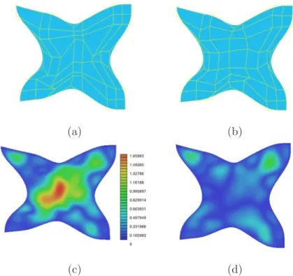
Two examples of r-refinement method are shown in Fig. 8 and Fig. 9. The initial B-spline parameterizations are presented in Fig. 8 (a) and Fig. 9 (a), Fig. 8 (b) and Fig. 9 (b) show the final parametrization obtained by r-refinement. The corresponding simulation error obtained from
22for initial and final parametrization are illustrated in Fig. 8(c), Fig. 9(c), Fig. 8(d) and Fig. 9
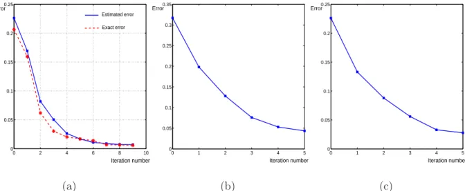
(d). From these two examples, we can find that by r-refinement method some inner control points are moved to the region with big error computed from (22). Quantitative data of r-refinement method presented in Fig.5, Fig.8 and Fig.9 are summarized in Table.2. Fig. 10 shows the error history during r-refinement for examples in Fig.5, Fig.8 and Fig.9. Table.2 and Fig. 10 illustrate that final parameterization of computational domain computed by r-refinement can achieve better accuracy with respect to the initial parameterization of computational domain.
Table 2: Quantitative data for r-refinement in Fig. 5, Fig.8and Fig.9. # deg.: degree of B-spline parameterization;
# con.: number of control points; # iter.: number of optimization iterations; einitial: estimated error for initial
parameterization; ef inal: estimated error for final parameterization.
Example # Deg. # Con. #Iter. einitial ef inal ef inal/einitial
Fig.5 3 28 9 0.226 7.08 × 10⁻³ 3.13%
Fig.8 3 64 5 0.317 4.36 × 10⁻² 13.75%
Fig.9 4 64 5 0.298 2.78 × 10⁻² 9.33%
7. Conclusion and future work
Parameterization of computational domains is the first step in an IGA process, and has some effect on simulation results. In this paper, we firstly propose constraint optimization method to parameterize the computational domains with good uniformity and orthogonality from the given four boundary planar B-spline curves. Then r-refinement method in isogeometric version is proposed to optimize the parameterization by repositioning the inner control points based on a posteriori error estimation. Examples and comparison are presented to show that the proposed methods can produce analysis-suitable parameterization of computational domain for IGA.
As part of the future work, we will generalize the proposed methods to 3D case, which is more important in practice. In particular, local r-refinement in IGA is our ongoing work for computational domain with complex geometry.
0 2 4 6 8 10 0 0.05 0.1 0.15 0.2 0.25 Iteration number Error Estimated error Exact error (a) 0 1 2 3 4 5 0 0.05 0.1 0.15 0.2 0.25 0.3 0.35 Iteration number Error (b) 0 1 2 3 4 5 0 0.05 0.1 0.15 0.2 0.25 Iteration number Error (c)
Fig. 10. Error history during r-refinement: (a) estimated error history (blue curve) and exact error history (red
curve) in Fig. 5; (b) estimated error history in Fig.8; (c) estimated error history in Fig.9.
Acknowledgements
The authors wish to thank all anonymous referees for their valuable comments and suggestions. The authors are supported by the 7th Framework Program of the European Union, project SCP8-218536 “EXCITING”. The first author is partially supported by the National Nature Science Foundation of China (No.61004117), the Zhejiang Provincial Natural Science Foundation of China under Grant No. Y1090718, and the Open Project Program of the State Key Lab of CAD&CG (A1105), Zhejiang University.
Appendix. Discrete Coons volume
The trivariate generalization of the method proposed in [21] can be used for parametric vol-ume generation from given boundary surfaces. For B-spline volvol-ume generation, the inner control points can be obtained by the linear combination of the boundary control points. Suppose that given boundary surfaces are B-spline surfaces, the opposite boundary B-spline surfaces have the same degree, number of control points and knot vectors. Given the boundary control points
c0,j,k, cl,j,k, ci,0,k, ci,m,k, ci,j,0, ci,j,n, (i = 0, . . . , l, j = 0, . . . , m, k = 0, . . . , n ), then the interior
ci,j,k = (1 − i/l)c0,j,k+ i/lcl,j,k+ (1 − j/m)ci,0,k+ j/mci,m,k
+(1 − k/n)ci,j,0+ k/nci,j,n− [1 − i/l, i/l]
c0,0,k c0,m,k cl,0,k cl,m,k 1 − j/m j/m −[1 − j/m, j/m] ci,0,0 ci,0,n ci,m,0 ci,m,n 1 − k/n k/n −[1 − k/n, k/n] c0,j,0 cl,j,0 c0,j,n cl,j,n 1 − i/l i/l +(1 − k/n) [1 − i/l, i/l] c0,0,0 c0,m,0 cl,0,0 cl,m,0 1 − j/m j/m +k/n [1 − i/l, i/l] c0,0,n c0,m,n cl,0,n cl,m,n 1 − j/m j/m
Then the corresponding B-spline volume has the following form σ(ξ, η, ζ) = l X i=0 m X j=0 n X k=0 ci,j,kNi(ξ)Nj(η)Nk(ζ).
where Ni(ξ), Nj(η) and Nk(ζ) are B-spline basis function with knot vectors given by boundary
surfaces.
References
[1] M. Aigner, C. Heinrich, B. J¨uttler, E. Pilgerstorfer, B. Simeon and A.-V. Vuong. Swept volume parametrization
for isogeometric analysis. In E. Hancock and R. Martin (eds.), The Mathematics of Surfaces (MoS XIII 2009), LNCS vol. 5654(2009), Springer, 19-44.
[2] M. Ainswort and J. Oden. A posteriori error estimation in finite element analysis. Wiley- Interscience, New York, 2002.
[3] F. Auricchio, L.B. da Veiga, A. Buffa, C. Lovadina, A. Reali, and G. Sangalli. A fully locking-free isogeometric approach for plane linear elasticity problems: A stream function formulation. Computer Methods in Applied Mechanics and Engineering, 197:160-172, 2007.
[4] Y. Bazilevs, L. Beirao de Veiga, J.A. Cottrell, T.J.R. Hughes, and G. Sangalli. Isogeometric analysis: approxi-mation, stability and error estimates for refined meshes. Mathematical Models and Methods in Applied Sciences, 6:1031-1090, 2006.
[5] Y. Bazilevs, V.M. Calo, T.J.R. Hughes, and Y. Zhang. Isogeometric fluid structure interaction: Theory, algo-rithms, and computations. Computational Mechanics, 43:3-37, 2008.
[6] Y. Bazilevs, V.M. Calo, Y. Zhang, and T.J.R. Hughes. Isogeometric fluid structure interaction analysis with applications to arterial blood flow. Computational Mechanics, 38:310-322, 2006.
[7] Y. Bazilevs, V.M. Calo, J.A. Cottrell, J. Evans, T.J.R. Hughes, S. Lipton, M.A. Scott, and T.W. Sederberg. Isogeometric analysis using T-Splines. Computer Methods in Applied Mechanics and Engineering, 199(5-8): 229-263, 2010.
[8] K.H. Brakhage and Ph. Lamby. Application of B-spline techniques to the modeling of airplane wings and numerical grid generation. Computer Aided Geometric Design, 25: 738-750, 2008.
[9] D. Burkhart, B. Hamann and G. Umlauf. Iso-geometric analysis based on Catmull-Clark subdivision solids. Computer Graphics Forum, 29(5): 1575-1584, 2010.
[10] W. Cao, W. Huang, and R.D. Russell. An r-adaptive finite element method based upon moving mesh PDEs. Journal of Computational Physics, 149, 221-244, 1999.
[11] G. Celniker and D. Gossard. Deformable curve and surface finite elements for free-form shape design. Computer Graphics (Procs of SIGGRAPH’91) 25(4): 257-266, 1991.
[12] E. Cohen, T. Martin, R.M. Kirby, T. Lyche and R.F. Riesenfeld, Analysis-aware Modeling: Understanding Quality Considerations in Modeling for Isogeometric Analysis. Computer Methods in Applied Mechanics and Engineering, 199(5-8): 334-356, 2010.
[13] J.A. Cottrell, T.J.R. Hughes, and A. Reali. Studies of refinement and continuity in isogeometric analysis. Computer Methods in Applied Mechanics and Engineering, 196:4160-4183, 2007.
[14] J.A. Cottrell, A. Reali, Y. Bazilevs, and T.J.R. Hughes. Isogeometric analysis of structural vibrations. Computer Methods in Applied Mechanics and Engineering, 195:5257-5296, 2006.
[15] T. Dokken, V. Skytt, J. Haenisch, K. Bengtsson. Isogeometric representation and analysis–bridging the gap between CAD and analysis. 47th AIAA Aerospace Sciences Meeting including The New Horizons Forum and Aerospace Exposition, 5-8 January 2009, Orlando, Florida.
[16] M. D¨orfel, B. J¨uttler, and B. Simeon. Adaptive isogeometric analysis by local h-refinement with T-splines.
Computer Methods in Applied Mechanics and Engineering, 199(5-8): 264-275, 2010.
[17] R. Duvigneau. An introduction to isogeometric analysis with application to thermal conduction. INRIA Research Report RR-6957, June 2009
[18] T. Elguedj, Y. Bazilevs, V.M. Calo, and T.J.R. Hughes. ¯Band ¯F projection methods for nearly incompressible
linear and non-linear elasticity and plasticity using higher-order NURBS elements. Computer methods in applied mechanics and engineering, 197: 2732-2762, 2008.
[19] J.A. Evans, Y. Bazilevs, I. Babuka, T.J.R. Hughes. n-Widths, supinfs, and optimality ratios for the k-version of the isogeometric finite element method, Computer Methods in Applied Mechanics and Engineering, 198: 1726-1741, 2009.
[20] G. Farin. Curves and Surfaces for Computer Aided Geometric Design: A Practical Guide, 5th Edition. Morgan Kaufmann, San Mateo, CA, 2001.
[22] J. Gain and N. Dodgson. Preventing self-Intersection under free-form deformation. IEEE Transactions on Visu-alization and Computer Graphics, 7(4), pp. 289-298, Oct.-Dec. 2001.
[23] P. Gill, W. Murray, M Wright. Practical Optimization. Springer, 1981.
[24] H. Gomez, V.M. Calo, Y. Bazilevs, and T.J.R. Hughes. Isogeometric analysis of the Cahn-Hilliard phase-field model. Computer Methods in Applied Mechanics and Engineering, 197:4333-4352, 2008.
[25] T.J.R. Hughes, J.A. Cottrell, Y. Bazilevs. Isogeometric analysis: CAD, finite elements, NURBS, exact geometry, and mesh refinement. Computer Methods in Applied Mechanics and Engineering 194, 39-41, pp 4135-4195, 2005. [26] T.J.R. Hughes, A. Realli, and G. Sangalli. Duality and unified analysis of discrete approximations in structural dynamics and wave propagation: Comparison of p-method finite elements with k-method NURBS. Computer methods in applied mechanics and engineering, 197: 4104-4124, 2008.
[27] T.J.R. Hughes, A. Realli, and G. Sangalli. Efficient quadrature for NURBS-based isogeometric analysis. Com-puter Methods in Applied Mechanics and Engineering, 199(5-8): 301-313, 2010.
[28] H. Kestelman. Mappings with non-vanishing Jacobian. Amer. Math. Monthly 78, 662-663, 1971.
[29] H.J. Kim, Y.D Seo and S.K Youn. Isogeometric analysis for trimmed CAD surfaces. Computer Methods in Applied Mechanics and Engineering, 198(37-40): 2982-2995, 2009.
[30] T. Martin, E. Cohen, and R.M. Kirby. Volumetric parameterization and trivariate B-spline fitting using harmonic functions. Computer Aided Geometric Design, 26(6):648-664, 2009.
[31] D.S. McRae. r-refinement grid adaptation algorithms and issues. Computer Methods in Applied Mechanics and Engineering, 189: 1161-1182, 2000.
[32] K. M. Morken. Some identities for products and degree raising of splines. Constructive Approximation, 7: 195-208, 1991.
[33] T. Nguyen, B. J¨uttler. Using approximate implicitization for domain parameterization in isogeometric analysis.
International Conference on Curves and Surfaces, Avignon, France, 2010.
[34] G. Xu, B. Mourrain, R. Duvigneau, A. Galligo. Optimal analysis-aware parameterization of computational domain in isogeometric analysis. Proc. of Geometric Modeling and Processing (GMP 2010), 2010, 236-254. [35] Y. Zhang, Y. Bazilevs, S. Goswami, C. Bajaj, and T.J.R. Hughes. Patient-specific vascular NURBS modeling for
isogeometric analysis of blood flow. Computer Methods in Applied Mechanics and Engineering, 196:2943-2959, 2007.