HAL Id: insu-00404734
https://hal-insu.archives-ouvertes.fr/insu-00404734
Submitted on 9 Mar 2021HAL is a multi-disciplinary open access archive for the deposit and dissemination of sci-entific research documents, whether they are pub-lished or not. The documents may come from teaching and research institutions in France or abroad, or from public or private research centers.
L’archive ouverte pluridisciplinaire HAL, est destinée au dépôt et à la diffusion de documents scientifiques de niveau recherche, publiés ou non, émanant des établissements d’enseignement et de recherche français ou étrangers, des laboratoires publics ou privés.
André Revil, Niklas Linde, Adrian Cerepi, D. Jougnot, S. K. Matthäi, S.
Finsterle
To cite this version:
André Revil, Niklas Linde, Adrian Cerepi, D. Jougnot, S. K. Matthäi, et al.. Electrokinetic coupling in unsaturated porous media. Journal of Colloid and Interface Science, Elsevier, 2007, 313 (1), pp.315 à 327. �10.1016/j.jcis.2007.03.037�. �insu-00404734�
Electrokinetic coupling in unsaturated porous media
A. Revil (1)*, N. Linde (2), A. Cerepi (3), D. Jougnot (1, 4), S. Matthäi (5), and S. Finsterle (6)
(1) CNRS-CEREGE-IRD, Université Paul Cézanne, Hydrogéophysique et Milieux Poreux, Aix-en-Provence, France (2) Swiss Federal Institute of Technology, Institute of Geophysics, Zurich, Switzerland
(3) Institut EGID, Université Michel de Montaigne Bordeaux III, Pessac, France (4) ANDRA, Chatenay-Malabry, France.
(5) Imperial College, Department of Earth Science and Engineering, London, United Kingdom
(6) Lawrence Berkeley National Laboratory, Earth Sciences Division, Berkeley, California, United States
* Also at CNRS-ANDRA / GDR FORPRO 0788, France and Colorado School of Mines, Colorado, United States.
___________________________________ Corresponding author:
André Revil,
CEREGE, Europôle de l'Arbois, BP 80, Cedex 4,
13545 Aix en Provence, France.
Phone +33-676-011-803
Running title: EK-COUPLING IN UNSATURATED MEDIA
Abstract. We consider a charged porous material that is saturated by two fluid phases that are immiscible and continuous at the scale of a representative elementary volume. The wetting phase for the grains is water and the non-wetting phase is assumed to be an electrically insulating viscous fluid. We use a volume averaging approach to derive the linear constitutive equations for the electrical current density as well as and the seepage velocities of the wetting and non-wetting phases at the scale of a representative elementary volume. These macroscopic constitutive equations are obtained by volume-averaging Ampère’s law together with the Nernst-Planck equation and the Stokes equations. The material properties entering the macroscopic constitutive equations are explicitly described as a function of the saturation of the water phase, the electrical formation factor, and parameters that describe the capillary pressure function, the relative permeability function, and the variation of electrical conductivity with saturation. New equations are derived for the streaming potential and electro-osmosis coupling coefficients. A primary drainage and imbibition experiment is simulated numerically to demonstrate that the relative streaming potential coupling coefficient depends not only on the water saturation, but also on the material properties of the sample as well as the saturation history. We also compare the predicted streaming potential coupling coefficients with experimental data from four dolomite core samples. Measurements on these samples include electrical conductivity, capillary pressure, the streaming potential coupling coefficient at various level of saturation, and the permeability at saturation of the rock samples. We found a very good agreement between these experimental data and the model predictions.
Keywords: Electro-osmosis, streaming potential, Stokes equation, Nernst-Planck equation, porous media, clay, saturation, capillary pressure.
1. Introduction
In a recent paper, Revil and Linde [1] derived linear constitutive equations of transport for a multi-component electrolyte saturating a porous material that undergoes reversible deformation. They used the excess of electrical charge in the pore space to model electrokinetic processes rather than the zeta-potential as traditionally done by most authors. Modeling based on the excess of charge has also been used to study the diffusion of ionic species in bentonite and clay-rocks, and to understand the streaming potential signals in the Callovo-Oxfordian clayrock of the Paris basin [2].
The model by Revil and Linde [1] was restricted to fully water-saturated materials. In this paper, we extend the electrokinetic part of their model to unsaturated porous materials under two phase flow conditions. We neglect the filtering effect associated with the transport of the ionic species, i.e., we model only the electrical current density and the seepage velocities of the wetting and wetting phases. We assume that the wetting phase for the solid is water and that the non-wetting phase is insulating (e.g., air or oil) and immiscible with the former. Both phases are assumed to be continuous at the scale of a representative elementary volume of the porous material.
There are many applications where models of electrokinetic processes that occur in unsaturated porous media are needed. In geosciences, examples include water transport in unsaturated parts of the porous soils [3, 4, 5], monitoring of the oil / water interface in reservoir engineering [6, 7], remediation (by electro-osmotic pumping) of soils contaminated by non-aqueous phase liquids (NAPLs) [8], monitoring of CO2 sequenstration in the ground, healing of
cracks of unsaturated clay-rocks by electro-osmotic pumping in civil engineering, and the study of diffusion of ionic species in unsaturated clay-rocks used as host formations for long-term storage of toxic wastes. To the best of our knowledge, our model is the first rigorous attempt to
derive the governing equations that describe the effect of water saturation upon streaming potential and electro-osmosis. A less rigorous derivation of the governing equation for streaming potentials in unsaturated media was recently presented by Linde et al. [9] who also compared laboratory experiments from a primary drainage experiment of a saturated sand column to new theory.
This paper is organized as follows. In Section 2, we present the reference state of an unsaturated porous material at rest in thermodynamic equilibrium. In Section 3, we describe the local equations (Nernst-Planck equation, Ampère's law, and Stokes equations) that govern transport of each fluid phase and electrical charges through the connected porous medium. In Section 4, we volume-average these local equations at the scale of a representative elementary volume. The final constitutive and continuity equations are summarized in Section 5. Hysteresis of the streaming potential coupling coefficient is illustrated in Section 6 by simulating a synthetic primary drainage and imbibition experiment. In Section 7, the predicted variation of the streaming potential coupling coefficients for different water saturations are compared with a set of experimental data made on dolomite rock samples.
2. The Reference State
We consider a charged stress-free porous material, where the surface of the grains has a fixed electrical charge. This fixed charge is counterbalanced by a countercharge located in the water saturated portion of the pore space (Figure 1). The charged porous medium is assumed to under thermodynamic equilibrium conditions. The porous material is saturated by two immiscible phases, a wetting phase (assumed to be water) and a non-wetting phase (assumed to an electrically insulating phase, such as air or oil). The water phase is assumed to be in thermodynamic equilibrium with an infinite reservoir of ions. This reservoir of ions include N different species (including possibly non-ionic species). The saturation of the water phase is
defined by 0 0 /
w w
s =V V, where 0 w
V (in m3) denotes the volume of the water phase in the
representative elementary volume, V (in m3). In the reference state, the volumetric fractions of
wetting (w) and non-wetting phases (n) with respect to the pore volume are written 0 w
s and 0 n
s , respectively. As only two fluids are present, we have the saturation condition:
1 0 0 + = n w s s . (1)
The water content in the reference state is 0 0 sw
θ = φ, where φ is the porosity.
The charge density QV sat, (in units of C m-3) is defined as the excess of charge per unit
pore volume at full water saturation [9, 10, 11]. We neglect the charge density that is associated with the interface between the wetting and the non-wetting phases, since it is small in comparison with the charge density associated with the pore water-solid interface [9]. The charge density
, V sat
Q is related to the concentration of species i per unit volume of water, C by the following i0
relationship 0 0 , 1 / N i i V sat w i q C Q s = =
∑
, (2)where QV sat, /s0w represents the excess of electrical charge per unit volume of water and qi is the
charge (in C) of the ionic species i. This means that the smaller the water saturation, the higher the volumetric charge density in the water saturated pore space of the medium (see Figure 1). The charge balance condition in the porous medium, prior to any disturbance, is
, 0 0 1 0 V sat sw s w w Q S Q s +V = , (3)
where Q is the total surface charge density (in C m-s 2) at the solid-water interface. This charge
density consists of the fixed charge density of the solid surface of the solid and the charge density of the Stern layer (see Figure 1). In Eq. (3), S (in msw 2) denotes the surface area of the
solid-water interface and 0 w
V (in m3) denotes the volume of the water phase in the representative
elementary volume. The solid and the non-wetting phases are assumed to be electrical insulators. However, because we include the Stern layer as part of the solid phase (Figure 1), the surface of the solid is conductive and is responsible for the so-called "surface conductivity" (e.g., [12, 13]).
The ionic concentrations in the pore water of the medium obeys the Boltzmann distributions (e.g., [2]), 0 0exp i 0 i i b q C C k T ϕ = − , (4)
where C is the average concentration of species i in the infinite reservoir of ions in local i0
equilibrium with the pore water contained in the charged porous medium, ϕ0 (in V) is the mean electrical potential in the water phase, kb is the Boltzmann constant (1.381 × 10⁻²³ J K-1), and T is
the absolute temperature of the medium (in K). The osmotic pressure in the water phase is defined by , p p 0w 0 w− = 0 π (5)
where p is the pressure of the wetting phase (in Pa) and w0 0 w
p is the pressure of the infinite
reservoir of ions (in Pa). The osmotic pressure is given by (e.g., [1, 2]),
(
)
∑
= − ≈ N i i i bT C C k 1 0 0 0 π , (6)The osmotic pressure is given by [1],
0 0 0 1 1 exp , N i b i i b q k T C k T ϕ π = = − − −
∑
(7)∑
= − = i b i i i w sat V T k q C q s Q 1 0 0 , exp ϕ . (8)Solving Eq. (8) for the mean electrical potential in the pore space given the charge density QV,sat
and the concentration of the ions in the ionic reservoir implies that the strength of the electrical potential ϕ0 when the water saturation decreases. In turn, an increase of the mean potential in Eq. (7) implies an increase of the osmotic pressure in the wetting phase.
The local electrical field in the pore water 0 0 =−∇ϕ w
E is mainly tangential to the surface of the grain surface (ns×E0w=0), where ns is the unit vector normal to S and directed from the sw
water to the solid phase. In the thermostatic state, there is no gradient of the electrochemical potentials of the ions in the pore space, i.e.,
0 0 0
0
b i i i w
k T∇C +q C E = . (9)
The equilibrium capillary pressure is defined by ( 0) 0 0 0 = − −π w n c p p p and it is a function
of the water saturation and the water saturation history.
3. Local Equations
We now consider the non-equilibrium situation in which the water and the non-wetting phases are moving through the porous medium. We first present the local constitutive equations in each phase ξ∈
{
s,w,n}
, where s, w, and n represent the solid, wetting, and non-wetting phases, respectively.3.1. Ampère’s Law
In the quasi-static limit of the Maxwell equations, the local Ampère's law is
ξ
ξ j
H =
×
∇ , (10)
The current density in the water phase j (in A m-w 2) is determined from the Nernst-Planck equation,
∑
= ∂ ∂ + + ∇ − = N i w w i i i i i b i w t C q b C Tb k q 1 u E j . (11)The mobilities bi (in N s m-1) entering Eq. (11) are related to the mobilities β
i (in m2 s-1 V-1)
used by Revil and Leroy [10] by bi=βi / qi and to the ionic self-diffusion coefficients Di used by Samson et al. [11] by Di =kbTbi.
The current density js of the solid phase is due to electrical conduction in the Stern layer coating the insulating grains. For clay materials, Leroy and Revil [12] and Leroy and Revil [13] presented a double layer model to determine the electrical conductivity associated with electro-migration of the ions in the Stern layer.
The boundary conditions at the interface S are sw
0 ) ( − = × s w s E E n , (12) 0 ( ) s× s− w =Qs s n H H v , (13) 0 ) ( − = ⋅ s w s j j n , (14)
where vs =∂us/∂t is the instantaneous velocity of the solid phase and u the displacement of s the solid phase.
The boundary conditions at the interface Snw separating the non-wetting phase and water
are 0 ) ( − = × n w n E E n , (15) n n w n n H H Q v n ×( − )= 0 , (16) 0 ) ( − = ⋅ n w n j j n , (17)
where n is the normal to n Saw directed from the water to the non-wetting phase, vn =∂un/∂t is the instantaneous velocity of the non-wetting phase and u is the displacement of the non-n wetting phase. We assume that the surface charge density at the interface between water and the non-wetting phase is negligible (see [9]), and therefore Q0n =0 and jn =0.
The concentration of the ionic species in the water phase, the local electrical field in the water phase, and the magnetic field in phase ξ are written as the sum of two terms,
i i i C c C = 0 + , (18) w w w E e E = 0 + , (19) ξ ξ ξ H h H = 0 + , (20)
where the first term represents the state variable in the reference state (see Section 2), while the second term represents a small deviation from this state caused by a pressure or electrical current disturbance.
As we neglect salt filtering associated with flow of the water phase (see [2] for the modeling of salt filtering effects at full water saturation), the average concentration perturbation is ci ≈0. In addition, we assume that there is no magnetic field in the thermostatic case and therefore Hξ0 =0 , Ampère’s law (Eq. 10) becomes ∇×hξ =jξ.
By keeping only the first-order leading terms in Eqs. (18)-(20) and using Eq. (9), the constitutive equation for the electrical current density in the pore fluid (see Eq. 11) becomes,
[
]
∑
= + + + ∇ − = N i w i w w i i i i i b i w q k Tb C bqC C 1 0 0 0 0 ) (E e v j , (21)(
)
∑
= + = N i w i w i i i i w q bqC C 1 0 0 v e j . (22)The boundary conditions for the electric and magnetic fields at the solid-water interface S are: sw
0 ) ( − = × s w s e e n , (23)
s S w s s h h Q v n ×( − )= 0 . (24)
The boundary conditions for the electric and magnetic fields at the interface of the two viscous phases Snw are 0 ) ( − = × n w n e e n , (25) 0 ) ( − = × n w n h h n . (26) 3.2. Mechanical Equations
The Stokes equations for the two fluid phases are
2 , ( / ) 0 e w w pw w QV sat sw w η ∇ v − ∇ +ρ g+ e = , (27) 0 2 −∇ + = ∇ vn n ng n p ρ η , (28)
where g is the gravitational acceleration vector, p is the pressure of the wetting phase including we
the osmotic pressure π, p is the pressure of the non-wetting phase, and n ηξ is the dynamic
viscosity of phase ξ. The terms ρwg and (QV sat, /s e represent the gravitational and w) w electrostatic body forces acting on the water phase. There is no electrostatic body force acting on the non-wetting phase since this phase is assumed to be insulating. The boundary condition for the displacement is us −uw =0 on S where sw u is the displacement of phase ξ ξ. On the interface Snw, the boundary condition un−uw=0 holds. We have pc = pn −(pw+π) where p c
is the capillary pressure.
4. Averaging the Local Equations
4.1. Volume-averaging approach
The local equations are now averaged at the scale of a representative elementary volume (REV) of the porous material. We define the REV as the volume of the porous material between
two large-parallel circular disks of area A (in m2) separated by the distance H (in m). This
corresponds to the case of a jacketed cylindrical sample in the laboratory. We assume that there are macroscopic potential differences between the two end-faces of the REV. The potential difference across the sample may be either a pressure difference ∆p of the two fluid phases or an
electrical potential difference ∆ψ. The unit vector normal to the end faces is denoted by z. By dividing this potential difference by H, one obtains the equivalent macroscopic field
perpendicular to the end-faces of the REV. We note z the unit vector normal to the end faces. The electrical field at the pore or grain scale obeys ∇ ×eξ =0 , so the electrical fields eξ can be derived from scalar electrical potentials eξ = −∇ψξ (we use the symbol ϕ to represent electrical potentials within the diffuse layer and the symbol ψ for the electrical potentials associated with the macroscopic electrical fields). The macroscopic electrical field is written as,
z⋅E = −∆ψ H , (29) ) 0 ( ) ( ξ ξ ψ ψ ψ = − ∆ H . (30)
In water, the fundamental Laplace problem is defined by (e.g., [14]),
0 2Γ = ∇ w , in Vw, (31) 0 = Γ ∇ ⋅ w s n , on Ssw, (32) 0 = Γ ∇ ⋅ w n n , on Snw, (33) = = = Γ 0 on , 0 on , z H z H w . (34)
The electrical potential in the water phase can be written as ψf = Γ∆ψ/ H and the electrical field by ew =−∇Γw∆ψ /H.
A similar boundary-value problem of the normalized effective potential Γn can be defined in the non-wetting phase by,
0 2Γ = ∇ n , in Vn, (35) 0 = Γ ∇ ⋅ n n n , on Snw, (36) = = = Γ 0 on , 0 on , z H z H n . (37)
The volume average of a quantity aξ (aξ is a scalar, a vector, or possibly a tensor) is,
aξ = 1
VV aξdV
ξ
∫
, (38)
where Vξ is the volume of the ξ-phase within the REV. Slattery's theorem [14] states that
dS V dS V S s w S n w w w nw sw a n a n a a =∇ +
∫
+∫
∇ 1 1 , (39) dS V S s s s s sw a n a a =∇ −∫
∇ 1 , (40) dS V S n n n n nw a n a a =∇ −∫
∇ 1 , (41)where dS is an infinitesimal surface volume element. The volumetric phase average and the volumetric total average are defined by (e.g., [14])
a ξ = aξ / fξ, (42) A = aξ ξ
∑
= fξa ξ ξ∑
, (43)where fξ is the volumetric fraction of phase ξ ( fs =1−φ is the volume fraction of the solid phase, fw =swφ is the volume fraction of water, and fn =(1−sw)φ is the volume fraction of the
non-wetting phase). This gives,
n w w w s s s A=(1−φ)a + φa +(1− )φa . (44)
The macroscopic laws of transport are obtained by using the following procedure (see [1, 14]): (1) volume-average the local equations, (2) use Slattery's theorem, (3) add the contributions from the solid and fluid phases, (4) apply boundary conditions, (5) introduce flow velocities relative to the water phase,
s w ws v v v = − , (45) n w wn v v v = − , (46)
and (6) apply the charge balance condition,
, 1 0 V sat sw s w w Q S Q s +V = . (47)
The microscopic Ampère law ∇×hξ =jξ derived in Section 3.1 is now volume-averaged in each phase of the porous continuum. This yields
s s S s s dS V sw j h n h − × = × ∇ 1
∫
, (48) w w S n w S s w dS V dS V nw sw j h n h n h + × + × = × ∇ 1∫
1∫
, (49) 0 1 × = − × ∇∫
dS V S n n n nw h n h . (50)Summing these three contributions yields
s w s w S s dS V sw j j h h n H+ × − = + × ∇ 1
∫
( ) , (51) J H= × ∇ , (52)s V s w j Q v j J= + −φ 0 . (53)
Eq. (53) follows from Eq. (51) by applying the boundary condition Eq. (24) and using the electroneutrality condition Eq. (47). The total current density J can be separated in two contributions,
S
c J
J
J= + , (54)
where J is the conductive current density associated with electro-migration of ions in pore c
water, while J is the streaming current density associated with the drag of the excess charge S
contained in the pore water by the flow (see [1] and [14] for the saturated case).
4.3. Volume-averaging the Conductive Current Density
We denote σw and σw the electrical conductivity of the pore water and the electrical
conductivity of a ionic reservoir in local equilibrium with the pore space of the medium, respectively. These two conductivities are defined by,
∑
= = N i i i i w q bC 1 0 2 σ , (55)∑
= = N i i i i w q bC 1 0 2 σ . (56)The difference between these electrical conductivities is given by Eq. (4). The average conductive current density is
∫
∫
+ = w s V w w V s s c dV V dV V e e J 1σ 1σ , (57) w w w s s c e s e J =(1−φ)σ + φσ , (58)phase is defined by E e w w α 1 = , (59)
∫
∫
⋅ Γ + ⋅ Γ + ≡ nw sw S w n w S w s w w dS V dS V z n z n 1 1 1 1 α , (60)where e is the phase average of the local electrical field in the water phase and w E=−z∆ψ/H
is the macroscopic electrical field. This macroscopic electrical field is also given by
n w s e e e E= + + , (61) n w w w s s e s e e E=(1−φ) +φ +φ(1− ) . (62)
The phase average of the electrical field e can also be related to the macroscopic electrical field n via the tortuosity of the non-wetting phase,
E e n n α 1 = , (63)
∫
⋅ Γ − ≡ nw S n n n n dS V z n 1 1 1 α . (64)We now connect the tortuosity of the pore space α (related to the definition of the electrical formation factor F at saturation by F =α/φ) with the tortuosities of the wetting and non-wetting phases. We define e as the local electrical field of the fluid phase, which is given by the f
weighted phase average of the electrical field in the wetting phase e and the phase average of w the electrical field in the non-wetting phase e by n
n w w w f s e s e e = +(1− ) . (65)
The electric field e f is related to the macroscopic field E by
E e α 1 = f . (66)
Combining Eqs. (59), (63), (65), and (66), we obtain n w w w s s α α α = + − 1 1 . (67)
It is seen that the tortuosity of the pore space is equal to the harmonic average of the tortuosities of each phase weighted by their relative saturation.
if we multiply Eq. (67) with the porosity, we can now relate the electrical formation factor to the tortuosities of the two fluid phases by,
n w w w s s F α φ α φ (1 ) 1 = + − . (68)
The electrical formation factor is often related to the porosity by a power-law function F=φ−m
(refereed to as Archie's first law [15]), and where 1 ≤ m ≤ 3 is called the cementation exponent
[15]. This cementation exponent can be considered as a fundamental textural property of the porous medium. The conductive current is written as,
[
w w w n]
w w w s c E s e s e s e J =σ −φ −φ(1− ) + φσ , (69)(
w s)
w w s n w s c E s e s e J =σ +φ σ −σ −(1− )φσ , (70)(
)
E J − − − + = s n w s w w w s c s s σ α φ σ σ α φ σ (1 ) . (71)The effective electrical conductivity of the porous material σ (S m-1) is defined by Ohm’s law, E Jc =σ , (72)
(
)
s n w s w w w s s s σ α φ σ σ α φ σ σ = + − −(1− ) . (73)to the Archie’s second law, w n w w w w s F s s σ σ α φ σ σ 1 lim 0 = = → , (74)
where n ≥ 1 is called the second Archie’s exponent or the saturation exponent (e.g., [16] and
references therein). We introduce now the second Archie’s exponent in the expression of the electrical conductivity by using the following change of variables
n w w w s F s ⇔ 1 α φ . (75)
We expect that a critical water saturation exists at which the water phase is no longer continuous. In this case, the tortuosity of the water phase goes to infinity and the transport of the ionic species through the pore water is no longer possible. To account for this phenomenon, we introduce a percolation threshold in the expression of the tortuosity of the water phase, which can be written as a function of the saturation of water and the tortuosity of the pore space according to 1/αw =(sw−swc)n−1/α as c w w s s ≥ and φ/αw =0 as c w w s
s ≤ . Note that this critical water saturation is not related to the residual water saturation, srw, to be introduced later, which has a
hydrodynamic meaning.
By using Eqs. (68), (73), and (75), we obtain the following expression for the electrical conductivity of the porous medium
[
w s]
n c w w s F s F σ σ σ = 1 ( − ) +( −1) . (76)This equation predicts that as long as the solid phase is continuous, the influence of the surface conductivity at the scale of the REV is not sensitive to the saturation of water. Eq. [76] (with
0 = c w
s ) was recently used by Linde et al. [17] to interpret jointly inverted cross-borehole radar and electrical resistivity geophysical data to determine transport properties of the sediments
between boreholes.
The Dukhin number is the ratio of the surface conductivity to the pore water conductivity [18]. We use Eq. (76) to define an effective Dukhin number at unsaturated conditions, Du*, as the ratio of the surface conductivity to the electrical conductivity of the pore space, which yields
w n c w w s s s F σ σ ) ( ) 1 ( Du* − − = . (77)
Here, the Dukhin number, Du*, is a power-law function of the water saturation, s . It increases w
strongly when the water saturation decreases, which describes the growing influence of surface conductivity at low water saturations. If we denote Du as the Dukhin number at full water saturation, Du* is related to Du by Du*=Du/(sw−scw)n.
4.4. Volume-averaging the Streaming Current Density
An expression for the average streaming current density in Eq. (54) is now derived
, 1 1 ( ) w N S i i w V sat s i V q C dV Q V = φ =
∫
∑
− J v v , (78) , ( ) S =φQV sat w− s J v v , (79) , V sat S w w Q s = J U , (80)where Uw =φsw(vw−vs)=φswvws is the Darcy or seepage velocity of the water phase. Eq. (80) predicts that the streaming current density is given by the excess charge density in the water phase times the seepage velocity of this phase. This formulation avoids the introduction of the zeta potential in describing the electrokinetic properties of porous media as done in most alternative models [3-7]. Our formulation emphasizes the role of the velocity of the water phase in playing a key-role in the electrokinetic properties of the porous material rather than focusing
on the pressure field of the water phase.
4.5. Volume-averaging the Stokes Equations
The boundary-value problem for the flow of the pore water through the porous material is defined by 2 , ( / ) w w pw w QV sat sw w η ∇ v = ∇ −ρ g− e , (81) 0 = ⋅ ∇ vw , (82) 0 = w v , on S , sw (83) = = ∆ = 0 on , 0 on , z H z p p , (84)
We separate the fluid velocity into mechanical (v ) and electrical (mw e w
v ) contributions and we assume that the velocities can be superimposed (see [14]) as
e w m w w v v v = + . (85)
The mechanical contribution to fluid flow can be recasted in terms of the fundamental Stokes problem, h m =∇ ∇2g , (86) 0 = ⋅ ∇ gm , (87) 0 = m g , on S and sw Snw, (88) h= H, at z=H 0, at z=0 . (89)
Both gm (in m2) and h (in m) are independent of the fluid properties. The electrical contribution
can be recast in terms of a similar fundamental Stokes problem where ∇h is replaced by ,
) ( g v w w w w m w p k ρ η φ =− ∇ − , (90) , e w V sat w w w k Q s φ η = v E , (91)
respectively. The permeability of the wetting phase (in m2) is defined by,
∫
⋅ − = w V m w w dV V s k φ z g . (92)The permeability of the wetting phase can be expressed as the product of the dimensionless relative permeability, kwr, and the absolute permeability of the porous medium, k k k
r w
w = . The
Darcy velocity of the wetting phase is given by,
, ( ) w V sat w w w w w w w k Q k p s ρ η η = − ∇ − + U g E. (93)
The last term of Eq. (93) accounts for electro-osmosis, that is; the flux of water moving through the porous medium in response to an applied electrical field. The term k Qw V sat, /ηw ws is therefore
an electro-osmotic coupling term.
A similar analysis for the non-wetting phase yields,
) ( g U n n n n n p k ρ η ∇ − − = . (94)
where kn =knrk, i.e., the permeability of the non-wetting phase. There is no electro-osmotic term
in Eq. (94) because the non-wetting phase is assumed to be insulating. Parametric equations providing relationships between r
w
k and r n
k as the function of the saturation of the water phase will be discussed in Sections 5 and 6 below. Note that if the medium is anisotropic, the permeability k of the porous material must be replaced by a second-order symmetric permeability tensor K.
5. Final Form of the Constitutive Equations
We now summarize the derived linear constitutive equations that apply at the scale of a REV of the porous medium. Using Eqs. (54), (72), (80), (93), and (94), the generalized form of the constitutive equations can be written in a matrix form as follows:
, ( V sat/ w) w w w n n Q s M p p ψ − ∇ = − ∇ ∇ J U U U , (95)
where M is a 3x3 square matrix of material properties,
, 0 0 /( ) / 0 0 0 / V sat w w w w w n n M Q k s k k σ η η η = . (96)
We have also pc = pn −(pw+π). If the osmotic pressure can be neglected, we recover the classical relationship for the capillary pressure pc = pn −pw. In the linear constitutive equations
(95), we have separated the convective and the non-convective terms. Another possibility is to explicitly write the convective term U in the first column of Eq. (95) in terms of pressure gradient alone, neglecting the influence of the other thermodynamic forces in this convective term. This approximation is valid near equilibrium where the pressure field is the leading term in the convective fluxes appearing in the first column of Eq. (95). In this case, the constitutive equations become ∇ ∇ ∇ − = n w n w p p L ψ U U J , (97)
, , /( ) 0 /( ) / 0 0 0 / V sat w w w V sat w w w w w n n Q k s L Q k s k k σ η η η η = . (98)
The matrix L is symmetrical ( L = L T), a property known as Onsager's reciprocity [19]. If the material is anisotropic, the tortuosity of the pore space and the permeability are second-order tensors with the same eigenvectors and each component of L is therefore a second-order tensor.
Two of the most popular parametric models to describe the influence of saturation on capillary pressure and relative permeability in numerical simulations are those of Brooks and Corey [20] and Van Genuchten [21]. For example, the Brooks and Corey relationships for the capillary pressure and the relative wetting and non-wetting fluid permeabilities are:
λ / 1 ) (s = p s− pc d , (99) λ λ)/ 3 2 ( ) (s =s + kwr , (100) ) 1 ( ) 1 ( ) (s = −s 2 −s(2+λ)/λ knr , (101) r w r w w s s s s − − = 1 , (102)
where p is called the displacement or capillary entry pressure, s denotes the effective water d
saturation, s is the residual saturation of the wetting phase, and wr λ is a curve-shape parameter corresponding to an index for the pore space distribution [20]. Typical values of λ vary from 1.70 for sands to 0.10 for clays [20]. So there are three textural exponents to consider in our model if we wan to use the Brooks and Corey relationships, n, m, and λ. A modified version of the van Genuchten model will be described in the following section. This model relies on additional parameters to account for hysteresis in the capillary pressure curve. The Brooks and Corey model is generally more adapted to porous materials with a narrow pore space distribution and therefore a finite displacement pressure while the Van Genuchten model is more appropriate to porous materials with a wide range of pore sizes.
In our model, the term L=QV sat, kw/(ηw ws ) corresponds to the streaming current coupling coefficient. Because the permeability of the water phase is hysteretic and depends non-linearly on the water saturation, a hysteretic behavior is also expected for the streaming current coupling coefficient. This is in contrast with the model proposed earlier by Revil and Cerepi [22], in which
L was assumed to be independent of saturation and the saturation history of the wetting phase.
The streaming potential (or voltage) coupling coefficient is defined by,
σ ψ L p C w − = ∂ ∂ ≡ =0 J , (103) , ( ) ( ) V sat w w w w w Q k s C s s η σ = − . (104)
The hysteretic behavior of the streaming coefficient coupling coefficient is explored in the next section. Note that the dependence of the coupling coefficient on saturation implied by Eq. (104) is somewhat similar to the equation empirically proposed by Perrier and Morat [4], who suggested that C is proportional to kw(sw)/σ(sw).
To complete the set of equations, we specify the continuity equations for the charge and the mass of each fluid phase. These macroscopic continuity equations are:
+ − ∂ ∂ − = ⋅ ∇ n w n w w w n w q q I s s t φρ φρ ) 1 ( 0 U U J , (105)
where I and qξ are the impressed electrical current and mass source rate of phase ξ, respectively. The combination of Eqs. (97) and (105) yields the governing equations to solve for any applications based on this theory. They yields a non-linear diffusion equation for the flow and a Poisson equation for the electrical potential.
6
. Numerical Simulations
To illustrate the model developed in the previous sections, we simulate numerically a primary drainage and secondary imbibition experiment of a horizontal sand column. This simulation will illustrate the relationship between the streaming potential coupling coefficient and water saturation. It will also demonstrate how hysteresis in the relative permeability function results in hysteresis in the streaming potential coupling coefficient. In this example, we only model the water phase by assuming that the non-wetting phase (air) is a passive bystander. We neglect the influence of entrapped air on the relative permeability of the non-wetting phase, which is in accordance with the assumption that the wetting and non-wetting phases are continuous at the scale of every representative elementary volumes of the system. However, entrapped air may have, in many real applications, entrapped air will have a significant influence on transport (see [23]).
Rather than using the Brooks and Corey model described in Section 5, the capillary pressure is modeled with a slightly modified version of the capillary pressure function of van Genuchten [21] as described in [23]: γ γ γ α n m r w r w r w w c s s s s p / 1 / 1 , 1 1 − − − − = − ∆ (106)
where s and wr swr,∆ are the residual water and satiated wate saturations, respectively, α , m, and n are curve shape parameters, and the superscript γ refers to drying (d) or wetting (w). The saturation swr,∆ is assumed to be dependent on the water saturation at which reversal from
drainage to imbibition occurs, sw∆:
) 1 ( 1 1 1 , ∆ ∆ ∆ − + − − = w nl w r w s R s s , (107)
r w r n nl s s R − − = 1 1 1 max , , (108)
where minimal satiated water saturation, snr,max, is an input parameter. We use this model to create a hysteretic capillary pressure function by choosing snmax<1, and by assigning different values for αd and αn, and nd and nw. The hysteresis in the relative permeability function is assumed to be a result of entrapment of air and is modelled with the modified Mualem model [24]. The amount of entrapped air is assumed to vary between zero and sgr
∆
with a linear dependence on the effective water saturation.
We consider a horizontally oriented cylinder with an inner diameter of 35 mm and a length of 1.27 m. This tube is open only at its two end-faces and filled with a porous sand, which is initially fully water-saturated. During the first 3.33 hours, we simulate a pumping of water at a constant rate of 54 ml/minute. Air is free to enter from the opposite end-face of the tube. This pumping phase is followed by a phase during which water is injected at the same steady rate during 2.22 additional hours.
The material properties of the material are taken to be relatively similar to the sand used for the experiment reported by [9]. The intrinsic permeability, k, is set to 8 × 10-12 m2 and the porosity, φ, is 0.34. The relative electrical conductivity was modeled with a non-hysteretic Archie’s second law, Eq. (74), with Archie’s second exponent n equal to 1. Significant hysteresis in the relative electrical conductivity function of sandstones has been reported from laboratory experiments when using deionized pore water [25], which may be explained by surface conductivity at the air-water interface. Using σw = 0.051 S m
-1
. For the simulation, this effect can be neglected. We will also neglect surface conductivity. We assigned r
w
s and r,max n
s equal to 0.2, 1/αd and 1/αn equal to 70 kPa and 35 kPa, respectively, nd and nw equal to 6 and 3, respectively. We made the common assumption in the van Genuchten model that mγ = 1-1 / nγ.
[27], respectively). We discretized the tube with a grid cell spacing of 0.5 mm and we neglected gravitational effects. The variation of relative electrical conductivity, capillary pressure, relative permeability, and the relative streaming potential coupling coefficient are displayed as a function of water saturation on Figure 2. In reference [22], the relative streaming potential coupling coefficient, Cr, is defined by,
sat r
C C
C ≡ . (109)
where C is the coupling coefficient at saturation sw and Csat is the streaming potential coupling
coefficient at full water saturation. We observe that the variation of the streaming potential coupling coefficient with the saturation of water displays an hysteresis. The relative coupling coefficient decreases almost linearly with the decrease of the water saturation and is equal to zero at the irreducible water saturation. We will show in Section 7 that this behavior agrees with the experimental data.
Using the previous material properties and their dependence with the saturation of the wetting phase, we simulate the distribution of the streaming potential ψ along the tube. We use the procedure described in [9] that is now summarized. We first simulate the hydraulic problem by neglecting the electro-osmotic contribution to the seepage velocity of the water phase. Then we solve the Poisson equation for the electrical potential ψ and resulting from Eqs. (95) and (105). Figure 3a shows profiles of the streaming potential 1 s after the drainage was initiated, 50 s before the drainage ended, and 500 s after the imbibition phase was initiated. The evolution of the streaming potential at the end of the tube is shown on Figure 3b (the reference electrode is placed at the opposite end-face of the tube). This shows that the polarity of the streaming potential is directly sensitive to the direction of flow at the entrance of the tube.
7
. Comparison with Experimental Data
In this section, we tested the derived equations for the streaming potential coefficient. According to Eqs. (99) to (104), the shape of the curve of the streaming potential coupling coefficient as a function of saturation is entirely determined (1) by the shape of the relative permeability versus saturation curve, (2) by the shape of the electrical conductivity versus saturation curve, and (3) by the saturation itself. Therefore, by measuring these parameters independently and inserting the results in Eq. (104), we can independently determine the saturation curve of the streaming potential coupling coefficient. This curve can then be compared with independent experimental evaluation of the streaming potential coupling coefficient at various saturations of the wetting phase.
7.1. Description of the Experiments
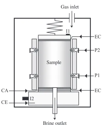
A set of four dolomite core samples (diameter 38 mm, length < 80 mm) were cored to perform the test. The measurements of two of these samples (E3 and E39) were already reported in [22] while the other measurements are new. Two thin sections representative of the texture of these samples are shown in Figure 4. They indicate a complex pattern of the pore space of these rocks. The petrophysical properties determined on these samples include the permeability at saturation, the resistivity index (at 1 kHz), the capillary pressure curves, and the streaming potential coupling coefficient at various saturation states. The “resistivity index” is defined by RI = ρ(sw)/ ρsat = σsat/ σ(sw) where ρ(sw) is the resistivity at the saturation sw and ρsat is the
resistivity when the porous medium is fully water-saturated. Petrophysical data of the core samples are reported in Table 1. The apparatus used to evaluate these properties is shown in Figure 5. For the resistivity measurements, an array of potential electrodes are located along the
sample. In addition, two current electrodes parallel are located at the end-faces of the sample. The electrodes are connected to an HP-impedancemeter (HP4263B) working in the frequency range 0.1–100 kHz.
Electrical resistivity measurements were performed at 1 kHz (4-electrode configuration). The brine used for all the electrical resistivity and streaming potential experiments contained 5 g L-1 NaCl (Cw = 8.6 - 10-2 Mol L-1, brine conductivity σw = 0.93 S m-1 at 25°C). The pH of the
solution in equilibrium with the medium was measured before and during the experiment. The pH is 8.0 at the beginning of the experiment and 8.3 ± 0.2 during the course of the experiment. The electrical resistivity index (measured at 1 kHz) was determined using the desaturation technique involving semi-permeable capillary diaphragms (ceramic membranes). The main advantages of this method are the reduction of capillary end effects and the ability to achieve a relatively uniform saturation distribution along the core length. Prior to the experiments, each sample was first dried for 48 hours at 50°C, then saturated with the brine under vacuum for 24 hours, and finally inserted (along with its jacket and the electrode pins into the pressurized cell (maximum confining pressure +3.0 MPa). Resistivities were measured at different saturations to determine the resistivity index RI at 1 kHz (Figure 5) .
In addition to the resistivity index, we also measured the permeability at saturation (from classical steady-state flow) and the irreducible water saturation from the capillary pressure curves (see Table 1). Hg-pressure curves (not shown here) indicated a complex pore structure with a wide spectrum of pore sizes. Finally, we measured the streaming potential coupling coefficient at different saturation states. The non-wetting phase used for the experiments is nitrogen.
In Figure 6, we report the dependence of the resistivity index, the capillary pressure, and the relative streaming potential coupling coefficients versus the saturation of the brine for sample #E3. We observe that the relative streaming potential coupling coefficient decreases when the water saturation decreases. The streaming potential coupling coefficient falls to zero when the
water saturation reaches the irreducible water saturation. Note the consistency of the irreducible water saturation resulting from the streaming potential measurements and from the capillary pressure curves (compare Figures 6b and 6c).
7.2. Comparison with the Model
We adopt the Brooks and Corey relationship for the permeability of the wetting phase and the capillary pressure (see Section 5). From Eqs. (76), (77), (100), (102), and (104), the streaming potential coupling coefficient becomes,
(
)
λ λ σ η / ) 3 2 ( 0 1 * Du 1 ) ( + − − + − − = r w r w w w n c w w w w V s s s s s s kF Q C . (110)From the electrical conductivity measurements, surface conductivity can be neglected, and therefore Du* << 1. As the mineral framework is well connected (Figure 3), we can expect that
0 ≈ c w
s (the water film around the grains is always above a percolation threshold even at very low water saturations). From Eq. (110), the coupling coefficient at saturation is given by
w w V sat kF Q C σ η 0 − = , (111)
and therefore from Eqs. (110) and (111), the coupling coefficient at saturation s is related to w
sat C by sat r w r w w n w C s s s s C λ λ)/ 3 2 ( 1 1 1 + + − − = . (112)
From Eqs. (109) and (112), the relative streaming potential coupling coefficient is therefore given by,
λ λ)/ 3 2 ( 1 1 1 + + − − = r w r w w n w r s s s s C . (113)
From Eq. (113), we have
1 lim 1 ≡ → r sw C , (114) 0 lim ≡ →s r s rC w w , (115)
as required for internal consistency of the model. In Equation (113), n is independently determined from the electrical conductivity curve and λ from the capillary pressure curve.
A comparison between the model and the experimental data is shown on Figure 6 for sample E3. In Figure 6a, we observe that the second Archie’s law reproduces well the resistivity data. This allows to determine the second Archie exponent n (2.7±0.2). In Figure 6b, we fit the capillary pressure curve with the Brooks and Corey parametric equation. This equation captures very well the shape of the curve. This gives the values of capillary entry pressure p (24±13 d
kPa), the residual saturation of the wetting phase s (0.36±02), and the index for the pore space wr
distribution λ (0.87±0.32).
Finally, we compare the prediction of Eq. (113) (in which all the parameters have been independently evaluated) with the experimental data in Figure 6c. The value of the coupling coefficient at saturation was extrapolated from the value obtained at various saturations (see Figure 7b). We obtain Csat ≈ -10-5 V Pa-1. Using Eq. (111), σw = 0.93 S m-1, and the values of the
parameters reported in Table 1, we obtain QV,sat = 9x10
3
C m-3. Then we use Eq. (109) with Csat
≈ -10-5 V Pa-1 to determine the values of the relative coupling coefficient as various saturation of
water. Eq. (113) agrees quite well with the experimental data. In Figure 7, we reported the whole data set of capillary pressure data and streaming potential coupling coefficients versus the saturation of the water phase. Clearly, our model is able to describe the sharp decrease of the coupling coefficient (over four orders of magnitudes) with the decrease of the water saturation for
full saturation to saturation close to the irreducible water saturation.
8
. Concluding Statements
The linear constitutive equations describing the electrokinetic coupling (streaming potential and electro-osmosis) of a charged deformable porous material under two-phase flow conditions have been derived using a volume-averaging approach. The model was derived assuming that the two fluid phases are continuous at the scale of a representative elementary volume of the porous material and that the viscous drag between the two fluid phases is negligible. This formulation is combined with classical parametric formulations describing the capillary pressure and the relative permeability functions as a function of the saturation of the wetting phase. The saturation history can be accounted for through the use of a modifier van Genuchten formulation for the capillary pressure curve.
The complete derivation presented in here complements the experimental work reported by Linde et al. [9], where it was shown that the present theory can predict the fluctuation of the streaming potential during the primary drainage of a vertical sand column. In a future contribution, we will use our model to assess the efficiency of electro-osmotic pumping to control the migration of NAPLs in the saturated and unsaturated zone. In addition, we plan to extend this model by incorporating diffusional effects in the constitutive equations to study diffusion of ions under unsaturated conditions (see also [11]).
Acknowledgments. This work is supported by the CNRS (The National Center for Scientific Research in France), ANDRA (The French National Agency for Radioactive Waste Management), the GDR FORPRO (Research Action Contribution FORPRO-2006/ ), and ANR-ECCO-PNRH (project POLARIS). We especially appreciate the support from Scott Altmann and Daniel Coelho from ANDRA and Joël Lancelot from GDR FORPRO for their helps
References
[1] A. Revil, N. Linde, J. Colloid Interf. Science 302 (2006) 682-694.
[2] P. Leroy, A. Revil, D. Coelho, J. Colloid Interf. Science 296 (2006) 248-255. A. Revil, P. Leroy, K. Titov, J. Geophys. Res. 110 (2005), doi: 10.1029/2004JB003442, B06202.
[3] C. Doussan, L. Jouniaux, J.-L. Thony, J. Hydrol. 267 (2002) 173-185.
[4] F. Perrier, P. Morat, Pure Appl. Geophys. 157 (2000) 785-810. [5] M. Darnet, G. Marquis, J. Hydrol. 285 (2004) 114-124.
[6] J.H. Saunders, M.D. Jackson, C.C. Pain, Geophys. Res. Lett. 33 (2006), doi:10.1029/2006GL026835, L15316.
[7] J. Singer, J. Saunders, L. Holloway, J.B. Stoll, C. Pain, W. Stuart-Bruges, G. Mason, Petrophysics 47(5) (2006) 427-441.
[8] J.Y. Wang, X.J. Huang, J.C.M. Kao, O. Stabnikova, J. Hazard. Mater. 136 (3) (2006) 532-541. J.H. Chang, Y.C. Liao, J. Hazard. Mater. 129 (1-3) (2006) 186-193. C. Yuan, Water Sci.
Technol. 53(6) (2006) 91-98.
[9] N. Linde, D. Jougnot, A. Revil, S. Matthäi, T. Arora, D. Renard, C. Doussan, Geophys. Res. Lett. 34 (2007), L03306, doi:10.1029/2006GL028878.
[10] A. Revil, P. Leroy, J. Geophys. Res. 109 (2004), doi: 10.1029/2003JB002755, B03208.
[11] E. Samson, J. Marchand, K.A. Snyder, J.J. Beaudoin, Cement Concrete Res. 35 (2005) 141-153.
[12] A. Revil, P. Leroy, Geophys. Res. Lett., 28(8) (2001) 1643-1646.
[13] P. Leroy, A. Revil, J. Colloid Interf. Science 270(2) (2004) 371-380. [14] S. Pride, Phys. Rev. B 50 (1994) 15,678-15,696.
[16] M.H. Waxman, L.J.M. Smits, Soc. Petrol. Eng. J. 8 (1968) 107-122. A. Revil, L.M. Cathles, S. Losh, J.A. Nunn, J. Geophys. Res., 103(B10) (1988) 23,925-23,936.
[17] N. Linde, A. Binley, A. Tryggvason, L. B. Pedersen, A. Revil, Water Resour. Res. 42
(2006), doi:10.1029/2006WR005131, W12404
[18] S.S. Dukhin, B.V. Derjaguin, in: E. Matievich (Ed.), Surface and Colloid Science, Wiley– Interscience, New York, 1974.
[19] J.R. Looker, S.L. Carnie, Transport Porous Med., 65 (1) (2006) 107-131.
[20] R.H. Brooks, A.T. Corey, Hydraulic properties of porous media, Hydrol. Pap. 3, Colorado State University (1964). R. H. Brooks, A. T. Corey. J. lrrig. Drain. Div. Am. Soc. Civ. Eng.,
92(IR2) (1966) 61-88.
[21] M.T. van Genuchten, Soil Sci. Soc. Am. J. 44 (1980) 892–898.
[22] A. Revil, A. Cerepi (2004), Geophys. Res. Lett. 31(11) (2004), L11605, doi:1029/2004GL020140.
[23] S. Finsterle, T. O. Sonnenborg, B. Faybishenko, Proceedings of the TOUGH workshop ’98,
Lawrence Berkeley National Laboratory Report LBNL-41995 (1998), 250-256. [24] R. J. Lenhard, J. C. Parker, Water Resour. Res., 23(12) (1987), 2197-2206. [25] R. Knight, Geophysics 56(12) (1991), 2139-2147.
[26] K. Pruess, C. Oldenburg, and G. Moridis, TOUGH2 user’s guide, version 2.0, Report
LBNL-43134 (1999), Lawrence Berkeley National Laboratory, Berkeley, California.
Table 1. Physical Properties of the Four Dolomite Samples. Sample k (mD) F m n s wr ρ (kg m-3) φ E3 48.4 21.8 1.93 2.7 0.42 1910 0.203 E39 23.8 96.1 2.49 3.5 0.40 2260 0.159 E35 - 52.1 2.12 2.6 0.54 2130 0.155 E24 - 19.67 1.55 4.2 0.62 2234 0.146
Captions
Figure 1. Sketch of the distribution of the ionic species in the pore space of a charged porous medium. The Stern layer of sorbed counterions is considered to be part of the solid. We denote
, /
V V sat w
Q =Q s the volumetric charge density of the pore space, and nS and nn the unit vectors
normal to the solid/water interface and to the water/air interface, respectively. We denote M+ as the metal counterions and A- the co-ions. The surface sites of both the solid/water and water/air interfaces are negatively charged and X- corresponds to the negative sites. a. At high water saturations, the excess charge density of the pore water is relatively low. b. At low water saturations, the counterions are packed in a smaller volume and therefore the effective excess charge density of the pore water is higher.
Figure 2. Results from a synthetic primary drainage experiment of an initially saturated sand column followed by imbibition. a. Relative electrical conductivity (dimensionless) versus water saturation. b. Capillary pressure curve. c. Relative permeability curve. d. Resulting relative streaming potential coupling coefficient versus water saturation. The relative coupling coefficient is defined by Cr =C/Csat where Csat is the coupling coefficient of the porous material fully saturated.
Figure 3. Results from a synthetic primary drainage experiment of a saturated sand column followed by secondary imbibition. a. Sketch of the experiment. The streaming potential (SP) is measured between a reference electrode (Ref) and a scanning electrode along the inner surface of
a plastic tube in which flow in unsaturated conditions occurred. b. Examples of the SP distributions throughout the tube at three time intervalls. b. Evolution of the simulated SP signal
between the end points of the column at three characteristic times (drainage ends and imbibition starts at 3.33 h).
Figure 4. Microstructure of the material (dolomite) investigated in this study (thin sections of Sample E39). Note the complex pattern of the microstructure and the wide distribution of pore
sizes. The total length of the micrographs is 150 µm.
Figure 5. Schematic diagram of the testing apparatus used to measure the resistivity index, the
capillary pressure, and the streaming potential. I1 and I2 are the current electrodes, P1 and P2 are the potential electrodes, CE a current electrode, and CA is a capillary plate, which corresponds to
a water-wet ceramic disc in epoxy resin, 5 mm-thick with a pore size of 150 µm.
Figure 6. Comparison between the three parametric equations discussed in the main text and experimental data for sample E3. a. Resistivity index (RI) versus brine saturation at 1 kHz. The
data are fitted with the second Archie’s law. b. Capillary pressure curve fitted with the Brooks and Corey model. This curve is used to define the irreducible water saturation. (the non-wetting
phase is nitrogen). c. Variation of the relative streaming potential coupling coefficient Cr versus
the water saturation. The solid line represents the predicted variation of Cr versus the water
saturation using the model developed in the main text. Note that there is no free parameter to fit here.
Figure 7. Capillary pressure and streaming potential coupling coefficient data for four samples investigated in this study. a. capillary pressure data. b. Streaming potential coupling coefficient
versus the saturation of water. Note the sharp decrease of the value of the coupling coefficient over four orders of magnitude.
Figure 1 X -X -X -M+ M+ M+ A -M+ X -X -M+ M+ A -M+ A -M+ X -X -X -X -X
-Clay basal surface
Stern layer Shear plane Bulk solution A -M+ M+ M+ M+ M+ M+ M+ Compact layer OHP Q0 Qβ Q Air X X X X X -M+ M+ M+ M+ V Ssw Ssw nn ns X -X -X -M+ M+ M+ A -M+ X -X -M+ M+ A -M+ A -M+ X -X -X -X -X
-Clay basal surface
Stern layer Shear plane Bulk solution A -M+ M+ M+ M+ M+ M+ M+ Compact layer OHP Q0 Qβ Q Air X X X X X -M+ M+ M+ M+ V Ssw Ssw nn ns
a. High water saturation
b. Low water saturation
A
Figure 2 0 0.2 0.4 0.6 0.8 1 0 0.2 0.4 0.6 0.8 1
Relative coupling coef
ficient Water Saturation(m) 0 0.2 0.4 0.6 0.8 1 0 0.2 0.4 0.6 0.8 1 Relative permeability Water Saturation(m) 0 0.2 0.4 0.6 0.8 1 0 20 40 60 80 100 Water Saturation(m) 0 0.2 0.4 0.6 0.8 1 0 0.2 0.4 0.6 0.8 1
Relative electrical conductivity
Water Saturation(m)
b. a.
d. c.