HAL Id: hal-02968286
https://hal.archives-ouvertes.fr/hal-02968286
Submitted on 16 Oct 2020
HAL is a multi-disciplinary open access
archive for the deposit and dissemination of
sci-entific research documents, whether they are
pub-lished or not. The documents may come from
teaching and research institutions in France or
abroad, or from public or private research centers.
L’archive ouverte pluridisciplinaire HAL, est
destinée au dépôt et à la diffusion de documents
scientifiques de niveau recherche, publiés ou non,
émanant des établissements d’enseignement et de
recherche français ou étrangers, des laboratoires
publics ou privés.
Distributed under a Creative Commons Attribution - NoDerivatives| 4.0 International
Tidally Forced Lee Waves Drive Turbulent Mixing
Along the Arctic Ocean Margins
Ilker Fer, Zoé Koenig, Igor Kozlov, Marek Ostrowski, Tom Rippeth, Laurie
Padman, Anthony Bosse, Eivind Kolås
To cite this version:
Ilker Fer, Zoé Koenig, Igor Kozlov, Marek Ostrowski, Tom Rippeth, et al.. Tidally Forced Lee Waves
Drive Turbulent Mixing Along the Arctic Ocean Margins. Geophysical Research Letters, American
Geophysical Union, 2020, 47 (16), pp.e2020GL088083. �10.1029/2020GL088083�. �hal-02968286�
Tidally Forced Lee Waves Drive Turbulent Mixing Along
the Arctic Ocean Margins
Ilker Fer1 , Zoé Koenig1,2 , Igor E. Kozlov3,4 , Marek Ostrowski5 , Tom P. Rippeth6 , Laurie Padman7, Anthony Bosse1,8 , and Eivind Kolås1
1Geophysical Institute, University of Bergen and Bjerknes Centre for Climate Research, Bergen, Norway,2Norwegian
Polar Institute, Tromsø, Norway,3Marine Hydrophysical Institute of RAS, Sevastopol, Russia,4Satellite Oceanography
Laboratory, Russian State Hydrometeorological University, Saint Petersburg, Russia,5Institute of Marine Research, Bergen, Norway,6School of Ocean Sciences, Bangor University, Bangor, UK,7Earth and Space Research, Corvallis, OR,
USA,8Now at Aix‐Marseille Université, Université de Toulon, CNRS/INSU, IRD, MIO, UM 110, Marseille, France
Abstract
In the Arctic Ocean, limited measurements indicate that the strongest mixing below the atmospherically forced surface mixed layer occurs where tidal currents are strong. However, mechanisms of energy conversion from tides to turbulence and the overall contribution of tidally driven mixing to Arctic Ocean state are poorly understood. We present measurements from the shelf north of Svalbard that show abrupt isopycnal vertical displacements of 10–50 m and intense dissipation associated with cross‐isobath diurnal tidal currents of∼0.15 m s−1. Energy from the barotropic tide accumulated in a trapped baroclinic lee wave during maximum downslopeflow and was released around slack water. During a 6‐hr turbulent event, high‐frequency internal waves were present, the full 300‐m depth water column became turbulent, dissipation rates increased by a factor of 100, and turbulent heatflux averaged 15 W m−2compared with the background rate of 1 W m−2.Plain Language Summary
Turbulent mixing in the Arctic Ocean water column affects sea ice variability through transport of subsurface heat toward the surface. This turbulent mixing is concentrated along the margins, mainly driven by tidalflow over sloping topography. However, processes of energy transfer from tides to turbulence in the Arctic are poorly understood, and the magnitudes and locations of mixing are poorly constrained. Here we present detailed measurements from the shelf north of Svalbard, showing a turbulent event driven by moderate tidal currents. The energy is trapped and accumulated at the time of maximum downslopeflow and is released at the turn of the tide when the entire water column becomes highly turbulent. Our observations imply that this process is an important source of mixing in the Arctic Ocean.1. Introduction
Much of the interior of the Arctic Ocean is quiescent (Fer, 2009; Lincoln et al., 2016), insulating the surface from heat imported into the Arctic Ocean by Atlantic Water intruding at intermediate depths (Carmack et al., 2015). In the Arctic basins, diapycnal heatfluxes out of this main oceanic heat source are weak (<1 W m−2) and typically driven by double diffusive convection (Polyakov et al., 2019; Shibley et al., 2017). However, in the critical region around Svalbard where warm water enters the Arctic Ocean, tides appear to play a key role in transporting this heat toward the surface. Mixing hotspots have been identified over regions of steep topography (Fer et al., 2010; Meyer et al., 2017; Padman & Dillon, 1991; Rippeth et al., 2015), where enhanced levels of turbulence cause diapycnal heatfluxes as large as 50 W m−2. The regions of energetic turbulent dissipation correspond with areas of conversion of barotropic tidal energy to barocli-nic waves and mixing (Fer et al., 2015; Padman & Dillon, 1991; Rippeth et al., 2015).
Planetary rotation constrains the conversion of barotropic tidal energy to freely propagating linear internal tides. For almost all of the major tidal constituents, most of the Arctic Ocean is poleward of their critical lati-tude,ϕc, the latitude at which the tidal frequency matches the local inertial period. In consequence, the lin-ear radiation pathway that the energy would normally follow from tides to dissipation, equatorward ofϕc, is not permitted (Falahat & Nycander, 2014; Musgrave, Pinkel, et al., 2016; Vlasenko et al., 2003). The hypothe-sized energy pathway at high latitudes is, instead, that the tidalflow over sloping topography induces a lee
©2020. The Authors.
This is an open access article under the terms of the Creative Commons Attribution License, which permits use, distribution and reproduction in any medium, provided the original work is properly cited.
RESEARCH LETTER
10.1029/2020GL088083
Key Points:
• Cross‐isobath diurnal currents generate nonlinear internal waves north of Svalbard
• Flow becomes supercritical during maximum off‐shelf tidal flow • Time‐averaged turbulent heat fluxes
increase by a factor of 4 when the turbulent period is included
Correspondence to:
I. Fer, ilker.fer@uib.no
Citation:
Fer, I., Koenig, Z., Kozlov, I. E., Ostrowski, M., Rippeth, T. P., & Padman, L., et al. (2020). Tidally forced lee waves drive turbulent mixing along the Arctic Ocean margins. Geophysical
Research Letters, 47, e2020GL088083. https://doi.org/10.1029/2020GL088083 Received 23 MAR 2020
Accepted 29 JUL 2020
wave, which is trapped and becomes unsteady as theflow becomes supercritical (Fer et al., 2015; Rippeth et al., 2017; Vlasenko et al., 2003), that is, Froude number Fr¼ u/c > 1, where u is the flow speed and c is the internal wave speed. The energy is dissipated locally and by breaking nonlinear internal waves (NLIWs) evolving with the changing phase of the tide (Rippeth et al., 2017).
The generation of NLIWs by the lee wave mechanism (e.g., Jackson et al., 2012; Maxworthy, 1979) occurs whenflow over sloping seabed vertically displaces the pycnocline. Over the upper slope and shelf edge, downslope (ebb)flow depresses the pycnocline, developing an initial lee wave (Sharples et al., 2007). The spatial scale of the generated wave is of the same order as the horizontal scale of the topographic feature, typically 5–30 km over the shelf edge. When Fr ¼ 1, the disturbance remains stationary, accumulates energy, and attains phase speed equal to theflow speed. As the flow slackens and Fr falls below 1, the wave propa-gates toward the generation region. Waves propagating on‐shelf steepen as they radiate into shallower water and further evolve and shorten (typically to about 1 km) as the tide turns, similar to internal hydraulic jumps that develop over steep slopes and deep‐ocean ridges after the maximum downslope flow and propagate upslope as theflow relaxes (e.g., Legg & Klymak, 2008; van Haren, 2019). The large vertical displacements of the density surfaces alter the sea surface roughness (Jackson et al., 2012), allowing the surface signature of NLIWs to be detected in remote sensing imagery (e.g., Alford et al., 2015; Jackson et al., 2012; Kozlov et al., 2017).
At midlatitudes, intense turbulence close to topography has been linked to tidal lee waves in deep sea envir-onments (Alford et al., 2015; Klymak et al., 2008; Li & Farmer, 2011; Musgrave, MacKinnon, et al., 2016), continental shelf breaks (Sharples et al., 2007) and in fjords (Cummins et al., 2003; Klymak & Gregg, 2003), and to lee waves associated with geostrophic flows (Thorpe et al., 2018). In the Arctic, Figure 1. Maximum tidal current speed (color) from Arc5km2018. Red contour is for the cross‐isobath component, |ux−
max|¼0.2 m s−1(i.e., strong tidal conversion potential). Isobaths (blue) are at 500, 1,000, and 1,500 m. Gray circle is the
critical latitudeϕcfor M2. The black outlined region north of Svalbard shows the domain of Figure 3, where the
observations were made. Abbreviated place names are YP, Yermak Plateau; ESS, Eastern Siberian Sea; CS, Chukchi Sea. The inset shows the probability distribution function (PDF) for Froude number calculated using |ux− max| and thefirst two baroclinic (evanescent) wave speeds for the K1wave frequency and the MIMOC August stratification at the
locations with |ux− max|>0.2 m s−1(inside red contours) and total water depth greater than 50 m.
10.1029/2020GL088083
Geophysical Research Letters
high‐frequency NLIWs have been observed in the eastern Arctic (Kurkina & Talipova, 2011; Morozov et al., 2017), including the northernflanks of the Yermak Plateau (Czipott et al., 1991; Padman & Dillon, 1991) (YP in Figure 1). The recent decline in Arctic seasonal sea ice has facilitated the mapping of the surface signa-tures of NLIWs from space using high‐resolution synthetic aperture radar (SAR), which shows the wide-spread occurrence of these features in the eastern Arctic Basin (Kozlov et al., 2017). Observations linking tides, NLIWs, and turbulence in the Arctic, however, are lacking despite their hypothesized importance in the magnitude and distribution of mixing.
Here we report detailed concurrent measurements of current structure, turbulence, and mixing in the Arctic Ocean that show intense dissipation of lee waves driven by the tidally induced stratified flow over sloping topography. We focus on the diurnal K1tidal current because it is directed approximately perpendicular to the shelf break at the study site, giving favorable forcing conditions for energy conversion. The aim of this paper is to identify the pathway of tidal energy to turbulence at a mixing hotspot in the Arctic, and to high-light the role of tidally‐forced mixing along the Arctic margins.
2. Data and Methods
Data were collected from R.V. Kristine Bonnevie during 27 June to 10 July 2018 using a conductivity ‐tem-perature‐depth (CTD) and lowered acoustic Doppler current profiler (LADCP) system, a vertical microstruc-ture profiler (VMP), a shipboard acoustic Doppler current profiler (SADCP), and a scientific echosounder (Simrad EK80). Observations presented here are from a 100‐km‐long transect across the shelf break at 18°E and from a 24‐hr process station near the 300‐m isobath. The CTD and LADCP profiles were obtained concurrently. The VMP was deployed immediately after the CTD/LADCP profiling. During the process sta-tion, a set of 4–5 VMP profiles (10–15 min between profiles) were taken, while the ship drifted about 0.5–1 km, after which there was a gap when the ship was repositioned. In addition, CTD/LADCP profiles were col-lected every 4 hr. The cruise data are available from Fer et al. (2020).
The CTD profiles were acquired using a Sea‐Bird Scientific, SBE 911plus system. Accuracies of the pressure, temperature, and salinity sensors are ±0.5 dbar, ±2 × 10⁻³°C, and ±3 × 10⁻³, respectively. The SADCP (150‐kHz Teledyne RDI Ocean Surveyor) velocity profiles (narrowband mode, 8‐m vertical bins) were pro-cessed into 3‐min averages using the University of Hawaii postprocessing software. The LADCP data (from two 300‐kHz Teledyne RDI Workhorse ADCPs attached to the CTD frame) were processed using the LDEO software version IX‐13 based on Visbeck (2002), using the constraints from ship navigation, bottom track-ing, and SADCP. Error in horizontal velocity measurements is less than 0.03 m s−1(Thurnherr, 2010). Microstructure measurements were made using the loosely tethered VMP2000 (Rockland Scientific International). The fall speed was 0.6 m s−1. The CTD data, averaged to 0.5 dbar, were taken from the pumped SBE‐CT sensor. Microscale velocity shear from shear probes was processed into 2‐dbar aver-aged dissipation rate estimates assuming isotropic turbulence,ϵ ¼ 7:5ν‾ ∂u′=∂zð Þ2, whereν is the viscosity (∼ 1.6 × 10⁻⁶m2s−1 for T¼ 3°C). The small‐scale shear variance (the term with the overline) was obtained by integrating the wavenumber spectrum of shear from half‐overlapping 2‐s segments in a wave-number range that is relatively unaffected by noise and corrected for the unresolved variance using the empirical model from Nasmyth (1970).
Acoustic data were collected using the EK80, operated in the narrowband mode at discrete frequencies. The volume backscatter data were reprocessed to remove noise and correct for spatial offsets and time delays between the transducers using the Large Scale Survey System (Korneliussen et al., 2016). Each of the EK80 frequencies displayed discrete targets across the water column and a continuous volume backscatter layer located midwater that followed the pycnocline variability. We used the acoustic image at 38 kHz, which best matched the isopycnal displacement pattern observed by the VMP profiles.
The squared buoyancy frequency was computed using N2¼ −(g/ρ0)∂σθ/∂z, where g ¼ 9.8 m s−2, ρ0¼ 1,027 kg−3, andσθis the potential density anomaly. Turbulent heatflux was obtained from FH¼ −ρ0Cp Kρ∂‾T=∂z, where ‾T is the background temperature profile, Cpis the specific heat capacity of seawater,
and the diapycnal eddy diffusivity was estimated from Kρ¼ 0.2ϵ/N2 (Gregg et al., 2018; Osborn, 1980).
Richardson number, Ri¼ N2/S2, at the time of a dissipation profile, was calculated using the 3‐min aver-aged velocity profile from the SADCP closest in time to the VMP cast. The vertical gradients of density in
10.1029/2020GL088083
Geophysical Research Letters
N2 and horizontal currents (u,v) in shear‐squared, S2¼ (∂u/∂z)2+ (∂v/∂z)2, were calculated at an 8‐m
vertical scale.
Surface manifestations of NLIWs were derived from optical Landsat‐8 and Sentinel‐1 A/B SAR images (Kozlov et al., 2015). We show the identified wave crests but not the actual images. We used Level 1 near‐infrared Band 5 and panchromatic Band 8 images from Landsat‐8, with spatial resolutions of 30 and 15 m, respectively, to detect NLIW signatures on 3 July 2018. We used Sentinel‐1A/B Level‐1 mediumreso-lution Ground Range Detected images taken in Extra Wide swath mode with a spatial resomediumreso-lution of 90 m to identify NLIWs during 4–5 July 2018.
We obtained tidal currents from Arc5km2018 (Erofeeva & Egbert, 2020), a barotropic inverse tidal model on a 5‐km grid. At each grid point, we predicted the total tidal current over a 30‐day window using all consti-tuents. We rotated the tidal currents to local along‐ and cross‐isobath components and calculated statistics of the total tidal current speed and cross‐isobath component.
The Froude number was computed as Fr¼ u/c, where u is the flow speed and c is the internal wave speed. We obtained the phase speeds of the subinertial evanescent response for the first (c1) and second (c2) Figure 2. Observations along the transect. (a) Distribution of dissipation rateϵ and isopycnals (0.02 kg m−3intervals). Arrowheads show the microstructure profiling locations. Bottom depth is from the ship's echosounder. The location of the process station is marked with a dashed line. The profiles were collected between 3 July 2018, 12:30 and 4 July 2018, 02:30 from shelf progressing toward deep water. (b) Wave crests identified from the SAR image obtained on 3 July 2018, 16:45, approximately when the station at 50 km was taken, about 1 hr before the profile at the process station. Position of the transect (line), the process station (pentagram), the isobaths at 250‐m intervals, and the coordinate system with the along‐isobath (x) and cross‐isobath (y) orientation are shown. The corresponding velocity
components are along‐isobath (ua, positive in x direction) and cross‐isobath (ux, positive downslope). (c) Depth‐averaged currents of ua(blue) and ux(red) from the SADCP (full lines, 1‐km horizontally averaged) and LADCP (circles).
(d) Froude number, Fr, using the depth‐averaged uxand the evanescent K1phase speeds for thefirst two
baroclinic modes at the process station.
10.1029/2020GL088083
Geophysical Research Letters
baroclinic modes by solving theflat‐bottom eigenvalue equation using the observed N(z) (e.g., Chapter 5, Phillips, 1977) and a relation above the critical latitude (Equation 2.10 in Musgrave, Pinkel, et al., 2016), with local f and K1wave frequency. For the time‐averaged N2profile at the process station, c1¼ 0.14 m s−1 and c2¼ 0.06 m s−1. Fits of the first two baroclinic modal shapes to the cross‐isobath baroclinic (depth‐average removed) currents and the pressure anomaly explained most of the variance (section 3). The second mode dominated the currents during the turbulent period.
To calculate Fr from tidal currents over the Arctic Ocean, we used the 30‐day maximum cross‐isobath tidal current, |ux− max|, and the evanescent wave phase speed for the K1frequency. We obtained the phase speeds of thefirst two baroclinic modes using the August stratification from the 0.5° resolution monthly isopycnal mixed‐layer ocean climatology (MIMOC; Schmidtko et al., 2013), linearly interpolated to the Arc5km2018 grid.
3. Results
In July 2018, sea ice melt resulted in strong ocean stratification north of Svalbard, with a buoyancy period of 20 min in the pycnocline at 50 m. Profiles collected along the transect showed a depression of isopycnals of about 50 m near the 300‐m isobath (Figure 2a). The transect started from the shelf on 3 July at 12:30 (all times are given in coordinated universal time UTC) and progressed north to deeper water, ending 4 July 02:30. The water column was highly turbulent near the 300‐m isobath (57 km), where ϵ reached 10−6W kg−1.
Current measurements were converted to along‐isobath, ua, and cross‐isobath, ux, components using the
orientation of the 500‐m isobath (60° counterclockwise from east; see Figure 2b). The large values of depth‐averaged uabetween 40 and 60 km mark the core of the warm boundary current (Figure 2c), whereas
the upslope (negative) values of uxare primarily from the diurnal tide, as will be shown later. Fr attains
near‐critical (Mode 1) and supercritical (Mode 2) values between 40 and 60 km along the transect. We detected signatures of NLIWs from the SAR image from 3 July 16:45, approximately when the station at 50 km with Fr > 1 was taken (Figure 2b). The ship returned to 57 km after the transect was completed to carry out detailed time‐series measurements (the process station).
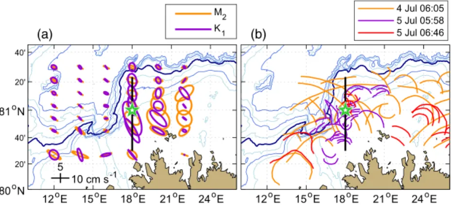
Tidal ellipses from Arc5km2018 are approximately normal to the isobaths, particularly for the diurnal con-stituent K1, giving favorable forcing conditions for energy conversion (Figure 3a). As we found for the dayof the transect, SAR images near the start and end of the process station show the presence of NLIWs (Figure 3b). The wave crests were densely spaced in the portion of the transect where theflow was observed to be critical or supercritical (see also Figure 2b). The location, however, is not unusually energetic, and such NLIWs are frequently detected in SAR images from the Arctic shelves (Kozlov et al., 2017).
Figure 3. (a) Tidal ellipses for the M2and K1constituents (on a coarse grid for clarity). (b) NLIW crests detected in SAR
images obtained during 4 and 5 July 2018. Position of the process station (pentagram) and the transect are marked. Isobaths (International Bathymetric Chart of the Arctic Ocean, IBCAO‐v3, Jakobsson et al., 2012) are drawn at 250‐m intervals with the 1,000‐m isobath emphasized.
10.1029/2020GL088083
Geophysical Research Letters
Figure 4. (a) Dissipation rateϵ, (b) uxfrom the SADCP (negative directed upslope), and (c) EK80 backscatter intensity. Arrowheads in panel (a) show the VMP
deployment times. Isopycnals (black) are at 0.02 kg m−3intervals. Bottom depth (gray) is from the ship's echosounder.
10.1029/2020GL088083
Geophysical Research Letters
The process station was occupied for 24 hr starting from 07:00 on 4 July, about 4 hr after the slope transect was completed. Repeat profiling revealed the strong variability of isopycnal depths and the highly intermit-tent nature of turbulence (Figure 4a). Isopycnal depth variations were consisintermit-tent with a dominant diurnal cycle but with substantial changes on shorter time scales. An abrupt depression of isopycnals was observed near 17:00, similar to the depression of the isopycnal surfaces observed at 17:00 the previous day at 300‐m depth (Figure 2a). The event was highly turbulent, withϵ ∼ 10−6W kg−1across the entire water column, similar to the profile taken 24 hr earlier (Figure 2a).
The vertical structure of the temporal variability in uxwas complex but showed the overall diurnal cycle
(Figure 4b). The turbulence event coincided with the slackening and reversal of ux. The downslope current
reached a subsurface peak of 0.3 m s−1approximately 1 hr before the isopycnal dip, and the current direction reversed in the short duration of the abrupt isopycnal perturbation (Figure 4b). The acoustic trace of the inter-nal wave observed in the midwater column with the EK80 (Figure 4c) was better temporally resolved than the other profiling measurements. In particular, the isopycnal dip of about 50 m near 17:00 at the time of the mid-waterflow reversal was more abrupt than could be resolved by the two consecutive microstructure profiles at that time. However, the EK80 data quality is compromised by the ship's drift and frequent repositioning by using propellers, and a detailed quantitative (e.g., spectral) or qualitative description is not possible. The depth‐averaged uxat the process station was dominated by the diurnal tide with amplitude 0.15 m s−1,
while uawas predominantly semidiurnal (Figure 5a). The observations are in reasonable agreement with the
Figure 5. (a) Depth‐averaged ua(blue), ux(red) from the SADCP (full lines, 30‐min moving averaged) and the LADCP (circles) and current vectors (upward arrow
is northwardflow). Dashed curves are the diurnal fit to ux(amplitude 0.15 m s−1, variance explained 93%) and the semidiurnalfit to ua(amplitude 0.04 m s−1,
variance explained 62%). Periods withflood (upslope flow), slack water, and ebb are marked. (b) Variance explained by the first two baroclinic modes fitted to ux. (c) Froude number, Fr, using the depth‐averaged |ux| and the evanescent K1phase speeds for thefirst two baroclinic modes.
(d) Dissipation averaged between 50 and 250 m (blue) and the fraction of the water column with Ri < 1 (red).
10.1029/2020GL088083
Geophysical Research Letters
predicted currents using Arc5km2018, with amplitudes within 5% for diurnals (1.5‐hr phase offset) and 20% for semidiurnals (not shown). During maximum ebb, the second baroclinic mode explained 90% of the cross‐isobath current structure and remained comparable to the first baroclinic mode at slack water (Figure 5b). The corresponding vertical structure can be seen in Figure 4b between 12:00 and 17:00. Coincident with the Mode 2 wave, Fr2was supercritical (Figure 5c), peaking during the maximum offslope flow accompanied by energetic turbulence (Figure 5d).
Dissipation rate averaged between 50 and 250 m increased by 2 orders of magnitude starting after the ebb maximum (after 12:00) until it decayed after the peak of theflood at 21:00 (Figure 5d). We chose this aver-aging depth range to minimize contributions from turbulence in the surface and bottom boundary layers; however, the pattern for the full‐depth averaged dissipation was similar. The onset of the turbulent event fol-lowed the supercritical conditions for Mode 2. At this time, the shear associated with the subsurface maxi-mum in ux(Figure 4b) reduced Ri. During the turbulent event, Ri < 1 in 40–90% of the water column, and
Ri < 0.25 in 10–30%, continuously for a period of 6 hr, despite the relatively coarse vertical resolution of the Ri estimates.
The mean temperature decreased with depth from 4.2°C near the surface to 2.6°C near the bottom, leading to typically negative values of turbulent heatflux, FH. The station‐averaged FHwas 4 W m−2directed
down-ward. Excluding the turbulent period between 13:00 and 19:00, the mean value of FHwas 1 W m−2. Over the
6‐hr turbulent period, the heat fluxes averaged 15 W m−2(standard deviation 7 W m−2) with some estimates exceeding 100 W m−2.
4. Discussion
Our observations are from a site north of Svalbard, where diurnal tides dominate cross‐isobath barotropic currents. The region experiences strong, tide‐modulated production of NLIWs and turbulence which increases the time‐averaged heat flux four times above the background values of 1 W m−2.
Conversion of barotropic tides to baroclinic waves will be strongest when the cross‐isobath component of barotropic tidal currents is largest. Energetic cross‐isobath tidal currents are common along the Arctic Ocean margins (Figure 1). Near‐critical or supercritical Froude numbers in these regions (Figure 1, inset) will allow trapping and unsteady evolution of lee waves and NLIWs. These calculations from the climatology likely underestimate the critical conditions (e.g., Fr inferred from the August climatology at the measure-ment location is 30% less than the value from observations). SAR images indeed show a widespread occur-rence of NLIWs in the eastern Arctic Basin (Kozlov et al., 2017).
We estimate the relative contribution of double‐diffusive and the tidally driven heat flux using the approximate surface area in the deep Canada (3 × 10¹²m2) and Eurasian (2 × 10¹²m2) basins and the areas with |ux− max|>0.2 m s−1(inside red contours above 74°N in Figure 1, 0.5 × 10¹²m2). The fraction of area covered by staircases and average double‐diffusive heat fluxes are summarized in Shibley et al. (2017). Using 0.3 W m−2 in 80% of the Canada Basin and 1 W m−2 in 25% of the Eurasian Basin, we obtain 1.2 × 10¹²W. If 15 W m−2(average over the turbulent event) occurs at 50% of the |ux− max| area (approximate probability of Fr2> 1 using the PDF from Figure 1), 25% of the time (based on our observa-tions), or a continuous 4 W m−2(our station average) over the same area, the Arctic‐wide contribution of the tides to the diapcynal heatflux is comparable to that due to double diffusion. This coarse estimate suggests that, despite the limited spatial extent and temporal occurrence of turbulent events, the contribu-tion of tidal‐driven mixing is substantial. Bulk estimates of heat loss from the Atlantic Water during its transformation from the Yermak Plateau to the Lomonosov Ridge (e.g., see Ivanov & Timokhov, 2019) suggest that of about 16 W m−2total heat loss, roughly 40% is released to the atmosphere, 40% warms the deeper water, and 20% is lost laterally. This implies the tidally driven mixing is an important compo-nent of this budget.
Along the Arctic Ocean margins, the pathway for the energy from the tide to turbulence is nonlinear and dominated by breaking unsteady lee waves and criticalflow. Here we have shown the enhanced turbulence associated with supercriticalflow of a trapped tidal lee wave. The vertical scale of sharp vertical undulations (10–50 m), duration (hours) and amplitude of bursts of dissipation (10−7to 10−6W kg−1), their vertical extent (100–400 m), and timing relative to the tidal currents (at the end of the ebb tide) are similar to
10.1029/2020GL088083
Geophysical Research Letters
observations from lower latitudes. In contrast to the lower latitudes where linear internal tidal waves disin-tegrate into packets of short NLIWs, linear response above critical latitudes is evanescent but nonlinear response has properties inherent to lee waves (at wavelengths comparable to the length scales of the bottom topography), independent of the rotation (Vlasenko et al., 2003).
The Arctic sea ice cover variability is sensitive to small changes in ocean‐ice heat flux (Carmack et al., 2015). Sea ice and stratification changes, e.g., reduced sea ice, weakening of the halocline, and shoaling of the intermediate‐depth Atlantic Water layer observed in the eastern Eurasian Basin (Polyakov et al., 2017, 2020) will affect the generation, radiation, and dissipation of the internal tide. The combination of these changes together with climate‐driven variability of the warm boundary current will alter both the mean flow and the internal wave speed, c. The polar regions are unique with relatively small values of c; hence, even modest tidal currents can lead to near‐critical states. For constant stratification, c scales as NH, where H is the total water depth. In the changing Arctic with weaker stratification, we expect smaller c, hence larger values of Fr. In turn, the transition toward near‐critical and supercritical states will be changed, altering the rate of tidal energy conversion, particularly through the nonlinear processes identified in this research. Understanding the pathway for the energy from tides to turbulence in the Arctic Ocean, the magnitude and distribution of the associated ocean mixing rates, and the role of feedbacks between mixing rates, strati fica-tion, sea ice, and the tide is key to predicting the fate of the Atlantic water in the Arctic and the evolution of the Arctic Ocean in a warming world.
Data Availability Statement
The Arc5km2018 tide model (Erofeeva & Egbert, 2020) is available at the Arctic Data Center (https://arctic-data.io/catalog/view/doi:10.18739/A21R6N14K). The Landsat and Sentinel data used in this study can be freely accessed from https://earthexplorer.usgs.gov/ and https://scihub.copernicus.eu, respectively. The cruise data are available from Fer et al. (2020), at the Norwegian Marine Data Centre (https://doi.org/ 10.21335/NMDC-2047975397), with Creative Commons Attribution 4.0 International License.
References
Alford, M. H., Peacock, T., MacKinnon, J. A., Nash, J. D., Buijsman, M. C., Centurioni, L. R., et al. (2015). The formation and fate of internal waves in the South China Sea. Nature, 521, 65–69. https://doi.org/10.1038/nature14399
Carmack, E., Polyakov, I., Padman, L., Fer, I., Hunke, E., Hutchings, J., et al. (2015). Towards quantifying the increasing role of oceanic heat in sea ice loss in the new Arctic. Bulletin of the American Meteorological Society, 96, 2079–2105. https://doi.org/10.1175/BAMS-D-13-00177.1
Cummins, P. F., Vagle, S., Armi, L., & Farmer, D. M. (2003). Stratified flow over topography: Upstream influence and generation of non-linear internal waves. Proceedings of the Royal Society of London, 459(2034), 1467–1487. https://doi.org/10.1098/rspa.2002.1077 Czipott, P. V., Levine, M. D., Paulson, C. A., Menemenlis, D. M., & Williams, R. G. (1991). Iceflexure forced by internal wave packets in the
Arctic Ocean. Science, 254, 832–835.
Erofeeva, S., & Egbert, G. (2020). Arc5km2018: Arctic Ocean Inverse Tide Model on a 5 kilometer grid, 2018. Dataset. https://doi.org/ 10.18739/A21R6N14K
Falahat, S., & Nycander, J. (2014). On the generation of bottom‐trapped internal tides. Journal of Physical Oceanography, 45, 526–545. https://doi.org/10.1175/JPO-D-14-0081.1
Fer, I. (2009). Weak vertical diffusion allows maintenance of cold halocline in the central Arctic. Atmospheric and Oceanic Science Letters,
2(3), 148–152.
Fer, I., Koenig, Z., Bosse, A., Falck, E., Kolås, E., & Nilsen, F. (2020). Physical oceanography data from the cruise KB2018616 with R.V. Kristine Bonnevie. Dataset. https://doi.org/10.21335/NMDC-2047975397
Fer, I., Müller, M., & Peterson, A. K. (2015). Tidal forcing, energetics, and mixing near the Yermak Plateau. Ocean Science, 11(2), 287–304. https://doi.org/10.5194/os-11-287-2015
Fer, I., Skogseth, R., & Geyer, F. (2010). Internal waves and mixing in the Marginal Ice Zone near the Yermak Plateau. Journal of Physical
Oceanography, 40, 1613–1630.
Gregg, M. C., D'Asaro, E. A., Riley, J. J., & Kunze, E. (2018). Mixing efficiency in the ocean. Annual Review of Marine Science, 10(1), 443–473. https://doi.org/10.1146/annurev-marine-121916-063643
Ivanov, V. V., & Timokhov, L. A. (2019). Atlantic Water in the Arctic Circulation Transpolar System. Russian Meteorology and Hydrology,
44(4), 238–249. https://doi.org/10.3103/S1068373919040034
Jackson, C. R., da Silva, J. C. B., & Jeans, G. (2012). The generation of nonlinear internal waves. Oceanography, 25(2), 108–123. https://doi. org/10.5670/oceanog.2012.46
Jakobsson, M., Mayer, L., Coakley, B., Dowdeswell, J. A., Forbes, S., Fridman, B., et al. (2012). The International Bathymetric Chart of the Arctic Ocean (IBCAO) version 3.0. Geophysical Research Letters, 39, L12609. https://doi.org/10.1029/2012gl052219
Klymak, J. M., & Gregg, M. C. (2003). The role of upstream waves and a downstream density pool in the growth of lee waves: Stratified flow over the Knight Inlet sill. Journal of Physical Oceanography, 33, 1446–1461.
Klymak, J. M., Pinkel, R., & Rainville, L. (2008). Direct breaking of the internal tide near topography: Kaena ridge, Hawaii. Journal of
Physical Oceanography, 38(2), 380–399.
10.1029/2020GL088083
Geophysical Research Letters
Acknowledgments
This work was part of the Nansen Legacy Program, Project Number 276730 funded by the Research Council of Norway. Analysis of satellite data performed by IEK was funded by RSF Grant No. 18‐77‐00082. TPR was sup-ported through the PEANUTS project, part of the Changing Arctic Ocean pro-gramme, jointly funded by NERC and BMBF. L. P. was supported by the U.S. National Science Foundation, Grant 1708424. The authors thank two anon-ymous reviewers for their critical com-ments and suggestions that improved the paper.
Korneliussen, R. J., Heggelund, Y., Macaulay, G. J., Patel, D., Johnsen, E., & Eliassen, I. K. (2016). Acoustic identification of marine species using a feature library. Methods in Oceanography, 17, 187–205. https://doi.org/10.1016/j.mio.2016.09.002
Kozlov, I. E., Kudryavtsev, V. N., Zubkova, E. V., Atadzhanova, O., Zimin, A. V., Romanenkov, D., et al. (2015). SAR observations of internal waves in the Russian Arctic seas. IEEE International Geoscience and Remote Sensing Symposium (IGARSS), 947–949. https://doi. org/10.1109/IGARSS.2015.7325923
Kozlov, I. E., Zubkova, E. V., & Kudryavtsev, V. N. (2017). Internal solitary waves in the Laptev Sea: First results of spaceborne SAR observations. IEEE Geoscience and Remote Sensing Letters, 14(11), 2047–2051. https://doi.org/10.1109/Lgrs.2017.2749681
Kurkina, O. E., & Talipova, T. G. (2011). Huge internal waves in the vicinity of the Spitsbergen Island (Barents Sea). Natural Hazards and
Earth System Sciences, 11(3), 981–986. https://doi.org/10.5194/nhess-11-981-2011
Legg, S., & Klymak, J. (2008). Internal hydraulic jumps and overturning generated by tidalflow over a tall steep ridge. Journal of Physical
Oceanography, 38(9), 1949–1964. https://doi.org/10.1175/2008jpo3777.1
Li, Q., & Farmer, D. M. (2011). The generation and evolution of nonlinear internal waves in the deep basin of the South China Sea. Journal
of Physical Oceanography, 41(7), 1345–1363. https://doi.org/10.1175/2011jpo4587.1
Lincoln, B. J., Rippeth, T. P., Lenn, Y.‐D., Timmermans, M. L., Williams, W. J., & Bacon, S. (2016). Wind‐driven mixing at intermediate depths in an ice‐free Arctic Ocean. Geophysical Research Letters, 43, 9749–9756. https://doi.org/10.1002/2016GL070454
Maxworthy, T. (1979). Note on the internal solitary waves produced by tidalflow over a 3‐dimensional ridge. Journal of Geophysical
Research, 84, 338–346. https://doi.org/10.1029/JC084iC01p00338
Meyer, A., Fer, I., Sundfjord, A., & Peterson, A. K. (2017). Mixing rates and vertical heatfluxes north of Svalbard from Arctic winter to spring. Journal of Geophysical Research, 122, 4569–4586. https://doi.org/10.1002/2016JC012441
Morozov, E. G., Kozlov, I. E., Shchuka, S. A., & Frey, D. I. (2017). Internal tide in the Kara Gates Strait. Oceanology, 57(1), 8–18. https://doi. org/10.1134/S0001437017010106
Musgrave, R. C., MacKinnon, J. A., Pinkel, R., Waterhouse, A. F., & Nash, J. (2016). Tidally driven processes leading to near‐field turbu-lence in a channel at the crest of the Mendocino Escarpment. Journal of Physical Oceanography, 46(4), 1137–1155. https://doi.org/ 10.1175/Jpo-D-15-0021.1
Musgrave, R. C., Pinkel, R., MacKinnon, J. A., Mazloff, M. R., & Young, W. R. (2016). Stratified tidal flow over a tall ridge above and below the turning latitude. Journal of Fluid Mechanics, 793, 933–957. https://doi.org/10.1017/jfm.2016.150
Nasmyth, P. W. (1970). Ocean turbulence (Ph.D. Thesis).
Osborn, T. R. (1980). Estimates of the local rate of vertical diffusion from dissipation measurements. Journal of Physical Oceanography,
10(1), 83–89.
Padman, L., & Dillon, T. (1991). Turbulent mixing near the Yermak Plateau during the coordinated Eastern Arctic Experiment. Journal of
Geophysical Research, 96(C3), 4769–4782.
Phillips, O. M. (1977). The dynamics of the upper ocean (2nd ed.). Cambridge, UK: Cambridge Univ. Press.
Polyakov, I. V., Padman, L., Lenn, Y. D., Pnyushkov, A., Rember, R., & Ivanov, V. V. (2019). Eastern Arctic Ocean diapycnal heatfluxes through large double‐diffusive steps. Journal of Physical Oceanography, 49(1), 227–246. https://doi.org/10.1175/Jpo-D-18-0080.1 Polyakov, I. V., Pnyushkov, A. V., Alkire, M. B., Ashik, I. M., Baumann, T. M., Carmack, E. C., et al. (2017). Greater role for Atlantic inflows
on sea‐ice loss in the Eurasian Basin of the Arctic Ocean. Science, 356, 285–291. https://doi.org/10.1126/science.aai8204 Polyakov, I. V., Rippeth, T. P., Fer, I., Alkire, M. B., Baumann, T. M., Carmack, E. C., et al. (2020). Weakening of cold halocline layer
exposes sea ice to oceanic heat in the eastern Arctic Ocean. Journal of Climate, 1–43. https://doi.org/10.1175/jcli-d-19-0976.1 Rippeth, T. P., Lincoln, B. J., Lenn, Y.‐D., Green, J. A. M., Sundfjord, A., & Bacon, S. (2015). Tide‐mediated warming of Arctic halocline by
Atlantic heatfluxes over rough topography. Nature Geoscience, 8(3), 191–194. https://doi.org/10.1038/ngeo2350
Rippeth, T. P., Vlasenko, V., Stashchuk, N., Scannell, B. D., Green, J. A. M., Lincoln, B. J., & Bacon, S. (2017). Tidal conversion and mixing poleward of the critical latitude (an Arctic case study). Geophysical Research Letters, 44, 12,349–12,357. https://doi.org/10.1002/ 2017GL075310
Schmidtko, S., Johnson, G. C., & Lyman, J. M. (2013). MIMOC: A global monthly isopycnal upper‐ocean climatology with mixed layers.
Journal of Geophysical Research: Oceans, 118, 1658–1672. https://doi.org/10.1002/jgrc.20122
Sharples, J., Tweddle, J. F., Green, J. A. M., Palmer, M. R., Kim, Y. N., Hickman, A. E., et al. (2007). Spring‐neap modulation of internal tide mixing and vertical nitratefluxes at a shelf edge in summer. Limnology and Oceanography, 52(5), 1735–1747.
Shibley, N. C., Timmermans, M. L., Carpenter, J. R., & Toole, J. M. (2017). Spatial variability of the Arctic Ocean's double‐diffusive staircase.
Journal of Geophysical Research: Oceans, 122, 980–994. https://doi.org/10.1002/2016JC012419
Thorpe, S. A., Malarkey, J., Voet, G., Alford, M. H., Girton, J. B., & Carter, G. S. (2018). Application of a model of internal hydraulic jumps.
Journal of Fluid Mechanics, 834, 125–148. https://doi.org/10.1017/jfm.2017.646
Thurnherr, A. M. (2010). A practical assessment of the errors associated with full‐depth LADCP profiles obtained using Teledyne RDI Workhorse acoustic Doppler current profilers. Journal of Atmospheric and Oceanic Technology, 27(7), 1215–1227. https://doi.org/ 10.1175/2010JTECHO708.1
van Haren, H. (2019). Off‐bottom turbulence expansions of unbounded flow over a deep‐ocean ridge. Tellus A: Dynamic Meteorology and
Oceanography, 71(1), 1653137. https://doi.org/10.1080/16000870.2019.1653137
Visbeck, M. (2002). Deep velocity profiling using lowered acoustic Doppler current profilers: Bottom track and inverse solutions. Journal of
Atmospheric and Oceanic Technology, 19(5), 794–807.
Vlasenko, V., Stashchuk, N., Hutter, K., & Sabinin, K. D. (2003). Nonlinear internal waves forced by tides near the critical latitude. Deep‐Sea Research Part I, 50(3), 317–338.