HAL Id: hal-00809220
https://hal.archives-ouvertes.fr/hal-00809220
Submitted on 8 Apr 2013
HAL is a multi-disciplinary open access
archive for the deposit and dissemination of
sci-entific research documents, whether they are
pub-lished or not. The documents may come from
teaching and research institutions in France or
abroad, or from public or private research centers.
L’archive ouverte pluridisciplinaire HAL, est
destinée au dépôt et à la diffusion de documents
scientifiques de niveau recherche, publiés ou non,
émanant des établissements d’enseignement et de
recherche français ou étrangers, des laboratoires
publics ou privés.
the Sphere : Application to the Fermi Gamma Ray
Space Telescope
Jérémy Schmitt, Jean-Luc Starck, J.M. Casandjian, Jalal M. Fadili, I. Grenier
To cite this version:
Jérémy Schmitt, Jean-Luc Starck, J.M. Casandjian, Jalal M. Fadili, I. Grenier. Multichannel Poisson
Denoising and Deconvolution on the Sphere : Application to the Fermi Gamma Ray Space Telescope.
Astronomy and Astrophysics - A&A, EDP Sciences, 2012, 546, 10 p. �10.1051/0004-6361/201118234�.
�hal-00809220�
Multichannel Poisson denoising and deconvolution
on the sphere : Application to the Fermi Gamma
Ray Space Telescope
J. Schmitt
1, J.L. Starck
1, J.M. Casandjian
1, J. Fadili
2, and I. Grenier
11
CEA, Laboratoire AIM, CEA/DSM-CNRS-Université Paris Diderot,
CEA, IRFU, Service d’Astrophysique, Centre de Saclay, F-91191 Gif-Sur-Yvette cedex, France 2
GREYC CNRS-ENSICAEN-Université de Caen, 6, Bd du Maréchal Juin, 14050 Caen Cedex, France
June 14, 2012
Abstract
A multiscale representation-based denoising method for spherical data contaminated with Poisson noise, the multiscale variance stabilizing transform on the sphere (MS-VSTS), has been previously proposed. This paper first extends this MS-VSTS to spherical two and one dimensions data (2D-1D), where the two first dimensions are longitude and latitude, and the third dimension is a meaningful physical index such as energy or time. We then introduce a novel multichannel deconvolution built upon the 2D-1D MS-VSTS, which allows us to get rid of both the noise and the blur introduced by the point spread function (PSF) in each energy (or time) band. The method is applied to simulated data from the Large Area Telescope (LAT), the main instrument of the Fermi Gamma-Ray Space Telescope, which detects high energy gamma-rays in a very wide energy range (from 20 MeV to more than 300 GeV), and whose PSF is strongly energy-dependent (from about 3.5˝ at 100 MeV to less than 0.1˝ at 10 GeV). Key words. Keywords should be given
Methods: Data Analysis, Techniques: Image Processing.
1. Introduction
1.1. Literature overview
The gamma-ray sky has been studied with unprecedented sensitivity and image capability thanks to the Large Area Telescope (LAT), the main instrument of the Fermi Gamma-Ray Space Telescope (Atwood et al. 2009), in an energy range between 20 MeV to greater than 300 GeV. The detection of gamma-ray point sources is difficult for two main reasons : the Poisson noise and the instrument’s point spread function (PSF). The Poisson noise is due to the fluctuations in the number of detected photons. Moreover, the effect of Poisson noise is strong because of the weakness of the fluxes of celestial gamma rays, especially outside the Galactic plane and far away from intense sources. The PSF width is strongly energy-dependent, varying from about 3.5˝ at 100
MeV to less than 0.1˝ (68% containment) at 10 GeV. Owing to large-angle multiple scattering in
the tracker, the PSF has broad tails, for which the 95%{68% containment ratio may be as large as 3.
An extensive literature exists on Poisson noise removal and the interested reader may refer to Schmitt et al. (2011) and Starck et al. (2010) for a thorough review. Motivated by new X-ray and gamma-ray data challenges, several restoration methods have been released in astrophysics that are based on wavelets (Movit 2009; Starck et al. 2009; Faÿ et al. 2011; Schmitt et al. 2010) or the Bayesian machinery (Conrad et al. 2007; Norris et al. 2010). Wavelets have also been used for source detection in Fermi data (Abdo et al. 2010), and a first Poisson denoising algorithm for spherical data was proposed in Schmitt et al. (2010). Starck et al. (2009) developed a denoising approach that effectively handles multichannel data acquired on a cartesian grid, and where the third dimension can be any physically meaningful index such as wavelength, energy, or time. While
traditional techniques integrate over all the third dimension in order to improve the signal-to-noise ratio (S/N) of the sources, their approach allows us to detect the sources while preserving all of their spectral information without sacrificing any the sensitivity. Nonetheless, none of these methods take into account the point spread function (PSF) of the instrument. Deconvolution can be very helpful in many situations such as source identification or flux estimation in the low energy bands where the resolution degrades severely. To the best of our knowledge, no general method for both multichannel denoising and deconvolving on the sphere has been developed in the literature. 1.2. Contributions
We propose a general framework for denoising and deconvolution that complies with all the above requirements, namely deals with
1. multichannel data, 2. acquired on the sphere,
3. and contaminated by Poisson noise.
Our approach builds upon the concept of variance stabilization applied to the spherical wavelet transform coefficients (Starck et al. 2006). This approach gives a multiscale representation of the Poisson data with variance-stabilized coefficients, which can be treated as if they were contaminated by a zero-mean white Gaussian noise. The developed algorithms are validated on simulated Fermi HEALPix multichannel cubes (nside “ 256) with energy bands ranging from 50 MeV to 50 GeV. 1.3. Paper organization
The rest of the paper is organized as follows. In section 2, we present a new wavelet transform for multichannel data on the sphere, and we show how the variance stabilization transform can be introduced into the decomposition. Section 3 details the way that this transform can be used for Gaussian and Poisson noise removal. Section 4 describes our deconvolution algorithm on the sphere for both mono-channel and multichannel spherical data. In Section 5, we finally draw some conclusions and give possible perspectives of this work.
1.4. Notations
For a real discrete-time filter whose impulse response is hris, ¯hris “ hr´is, i P Z is its time-reversed version. The discrete circular convolution product of two signals is written ‹, where the term circular represents periodic boundary conditions. The symbol δris is the Kronecker delta.
For the wavelet representation, the low-pass analysis filter is denoted h and the high-pass is taken as g “ δ ´ h throughout the paper. We denote the up-sampled version of h as hÒjrls “ hrls
if l{2j
P Z and 0 otherwise. We define hpjq“ ¯hÒj´1
‹ ¨ ¨ ¨ ‹ ¯hÒ1
‹ ¯h for j ě 1 and hp0q
“ δ.
The scaling and wavelet functions used for the analysis (respectively, synthesis) are denoted φ (with φpx2q “řkhrksφpx´kq, x P R and k P Z) and ψ (with ψpx2q “řkgrksφpx´kq, x P R and k P Z) (respectively, rφ and rψ).
2. Multiscale representation for multichannel spherical data with poisson noise
2.1. Fast undecimated 2D-1D wavelet decomposition/reconstruction on the sphere
Our goal is to analyze multichannel data acquired on a sphere with a non-isotropic two-and-one-dimensional (2D-1D) wavelet, where the two first dimensions are spatial (longitude and latitude) and the third dimension is either the time or the energy. Since the dimensions do not have the same physical meaning, it appears natural that the wavelet scale along the third dimension (energy or time) should not be connected to the spatial scale. Hence, we define the wavelet function as
ψpkθ, kϕ, ktq “ ψpθφqpkθ, kϕqψptqpktq, (1)
where ψpθφqis the spherical two dimensional (2D) spatial wavelet and ψptqthe one-dimensional (1D)
wavelet along the third dimension. Similarly to Starck et al. (2009), we consider only isotropic and dyadic spatial scales. We build the discrete 2D-1D wavelet decomposition by first taking a spherical 2D undecimated wavelet transform for each kt, followed by a 1D wavelet transform for each spatial
Hence, for a given multichannel data set on the sphere Y rkθ, kϕ, kts and after applying first the
2D spherical undecimated wavelet transform, we have the reconstruction formula
Y rkθ, kϕ, kts “ aJ1rkθ, kϕ, kts `
J 1
ÿ
j1“1
wj1rkθ, kϕ, kts, @kt, (2)
where J1is the number of spatial scales, aJ1 is the (spatial) approximation subband, and twj1u
J1
j1“1
are the (spatial) detail subbands. To simplify the notations in the sequel, we replace the two spatial indices by a single index kr, which corresponds to the pixel index. Equation (2) now reads
Y rkr, kts “ aJ1rkr, kts `
J 1
ÿ
j1“1
wj1rkr, kts, @kt. (3)
For each spatial location kr and each 2D wavelet scale j1, we then apply a 1D wavelet transform
along t on the spatial wavelet coefficients wj1rkr, ¨s such that
wj1rkr, kts “ wj1,J2rkr, kts `
J2
ÿ
j2“1
wj1,j2rkr, kts, @pkr, ktq, (4)
where J2 is the number of scales along t. The approximation spatial subband aJ1 is processed in a similar way, hence yielding
aJ1rkr, kts “ aJ1,J2rkr, kts `
J2
ÿ
j2“1
wJ1,j2rkr, kts, @pkr, ktq. (5)
Inserting Eqs. (4) and (5) into (3), we obtain the 2D-1D spherical undecimated wavelet represen-tation of Y : Y rkr, kts “ aJ1,J2rkr, kts ` J1 ÿ j1“1 wj1,J2rkr, kts ` J2 ÿ j2“1 wJ1,j2rkr, kts ` J1 ÿ j1“1 J2 ÿ j2“1 wj1,j2rkr, kts . (6)
In this expression, four kinds of coefficients can be distinguished: – Detail-detail coefficients (j1ď J1 and j2ď J2):
wj1,j2rkr, ¨s “ pδ ´ ¯h1Dq ‹ ph
pj2´1q
1D ‹ aj1´1rkr, ¨s ´ h
pj2´1q
1D ‹ aj1rkr, ¨sq. (7) – Approximation-detail coefficients (j1“ J1and j2ď J2):
wJ1,j2rkr, ¨s “ h
pj2´1q
1D ‹ aJ1rkr, ¨s ´ h
pj2q
1D ‹ aJ1rkr, ¨s. (8)
– Detail-approximation coefficients (j1ď J1 and j2“ J2):
wj1,J2rkr, ¨s “ h
pJ2q
1D ‹ aj1´1rkr, ¨s ´ h1DpJ2q‹ aj1rkr, ¨s. (9) – Approximation-approximation coefficients (j1“ J1and j2“ J2):
aJ1,J2rkr, ¨s “ h
pJ2q
1D ‹ aJ1rkr, ¨s. (10)
2.2. Multi-scale variance stabilizing transform on the sphere (MS-VSTS)
Schmitt et al. (2010) proposed a multiscale variance stabilizing transform adapted for Poisson spherical data. This transform was dubbed the multi-scale variance stabilizing transform on the Sphere (MS-VSTS). The MS-VSTS is a multi-scale decomposition method designed for Poisson noise that is based on a variance stabilizing transform(VST). Poisson noise is indeed signal-dependent, which complicates its removal. The aim of a VST is to get rid of this signal-dependence by transforming a Poisson distribution into a Gaussian distribution of known variance. In a nutshell, the MS-VSTS consists of plugging a VST into a multi-scale transform–the isotropic undecimated wavelet transform on the sphere (IUWTS)– in order to realize (approximately) Gaussian zero-mean
multiscale coefficients with constant variance. The noise on coefficients can then be easily removed using Gaussian denoising methods such as wavelet shrinkage, as we see in the next section.
The MS-VSTS scheme is defined recursively by inserting a (nonlinear) square-root VST into the IUWTS steps, that is
IUWTS " aj “ hj´1‹ aj´1 dj “ aj´1´ aj ùñ MS-VSTS (VST + IUWTS) " aj “ hj´1‹ aj´1 dj “ Tj´1paj´1q ´ Tjpajq , (11)
where Tj is the VST operator on scale j
Tjpajq “ bpjqsignpaj` cpjqq
b
|aj` cpjq|, (12)
with the VST constants bpjq and cpjq that depend solely on the filter h and the scale level j.
Zhang et al. (2008) showed that the MS-VSTS detail coefficients dj on locally homogeneous parts
of the underlying intensity signal follow asymptotically a zero-mean normal distribution with an intensity-independent variance that relies only on the filter h and the current scale j. Consequently, for a given h, both the stabilized variances and the constants bpjq and cpjq can be pre-computed
once and for all (Schmitt et al. 2010).
2.3. Multichannel MS-VSTS
We now extend the MS-VSTS machinery to the multichannel case. This amounts to plugging the VST into the spherical 2D-1D undecimated wavelet transform introduced in Section 2.1. This again gives rise to four types of coefficients that take the following forms:
– Detail-detail coefficients (j1ď J1 and j2ď J2):
wj1,j2rkr, ¨s “ pδ ´ ¯h1Dq ‹ ´ Tj1´1,j2´1 ´ hpj2´1q 1D ‹ aj1´1rkr, ¨s ¯ ´ Tj1,j2´1 ´ hpj2´1q 1D ‹ aj1rkr, ¨s ¯¯ . (13) – Approximation-detail coefficients (j1“ J1 and j2ď J2):
wJ1,j2rkr, ¨s “ TJ1,j2´1 ´ hpj2´1q 1D ‹ aJ1rkr, ¨s ¯ ´ TJ1,j2 ´ hpj2q 1D ‹ aJ1rkr, ¨s ¯ . (14)
– Detail-approximation coefficients (j1ď J1 and j2“ J2):
wj1,J2rkr, ¨s “ Tj1´1,J2 ´ hpJ2q 1D ‹ aj1´1rkr, ¨s ¯ ´ Tj1,J2 ´ hpJ2q 1D ‹ aj1rkr, ¨s ¯ . (15)
– Approximation-approximation coefficients (j1“ J1 and j2“ J2):
aJ1,J2rkr, ¨s “ h
pJ2q
1D ‹ aJ1rkr, ¨s. (16)
In summary, all 2D-1D wavelet coefficients twj1,j2uj1ďJ1,j2ďJ2 are now stabilized, and the noise in all these wavelet coefficients is a zero-mean Gaussian with known variance that depends solely on h on the resolution levels pj1, j2q. As before, these variances can be easily tabulated.
3. Application to multichannel denoising
We define X to be the noiseless data and Y their observed noisy version. In the case of the additive zero-mean white Gaussian noise, we have Y „ N pX, σ2
q, and for the Poisson noise Y „ PpXq. The main objective behind denoising is to estimate X from Y .
3.1. Warm-up: Gaussian noise
We start with the simple and instructive case where the noise in Y is additive white Gaussian. As the spherical 2D-1D undecimated wavelet transform described in Section 2.1 is linear, the noise remains Gaussian in the transform domain. Therefore, the thresholding strategies that have been developed for wavelet Gaussian denoising can be applied to the spherical 2D-1D wavelet
transform. Denoting the thresholding operator as TH, the denoised 2D-1D estimate of X obtained by thresholding the wavelet coefficients in Eq. (6) reads
r Xrkr, kts “ aJ1,J2rkr, kts` J1 ÿ j1“1 THpwj1,J2rkr, ktsq` J2 ÿ j2“1 THpwJ1,j2rkr, ktsq` J1 ÿ j1“1 J2 ÿ j2“1 THpwj1,j2rkr, ktsq. (17) A typical choice of TH is the hard thresholding operator parametrized by the scalar threshold τ ě 0, i.e.
THpxq “"0 if |x| ă τ,
x otherwise. (18)
The threshold τ is typically chosen to be between three and five times the noise standard deviation. 3.2. Poisson noise
The treatment of Poisson noise is far more complicated than its Gaussian counterpart, the main reason being that the noise variance is equal to its mean. This is where the MS-VSTS comes into play. The role of the MS-VSTS is indeed to get rid of this dependence of the variance on the mean by ensuring that the transformed coefficients are Gaussian with constant variance (without loss of generality, this variance can be assumed to be equal to 1). In other words, after the MS-VSTS, we are brought to a Gaussian denoising problem where standard thresholding approaches apply.
Nevertheless, denoising is not straightforward because there is no explicit reconstruction for-mula available because of the form of the non-linear stabilization equations above. Formally, the stabilizing operators Tj1,j2and the convolution operators along the spatial and the third dimensions do not commute, even though the filter bank satisfies the exact reconstruction formula. To circum-vent this difficulty, we propose to solve this reconstruction problem by advocating an iterative reconstruction scheme.
3.3. Iterative reconstruction
We define W to be the transform operator associated with the 2D-1D IUWTS described in Section 2.1, and R to be its inverse transform. We define M to be the multiresolution support, which is determined by the set of significant coefficients detected among WY at each scale pj1, j2q
and location pkr, ktq, i.e.
M “ tpj1, j2, kr, ktq
ˇ
ˇpWY qj1,j2rkr, kts is significantu. (19) We define M to be the orthogonal projector onto M, i.e. @d
pMdqj1,j2rkr, kts “ "
pWY qj1,j2rkr, kts if pj1, j2, kr, ktq P M, dj1,j2rkr, kts otherwise.
(20)
Our goal is to seek a solution rX that preserves the significant structures of the original data by reproducing exactly the same wavelet coefficients as those of the input data Y , but only on scales and at positions where significant coefficients have been detected. Furthermore, as Poisson intensity functions are positive by nature, a positivity constraint is imposed on the solution. It is clear that there are many solutions satisfying the positivity and multiresolution support consistency requirements, e.g. Y itself. Thus, our reconstruction problem based solely on these constraints is an ill-posed inverse problem that must be regularized. Typically, the solution in which we are interested must be sparse by involving the lowest budget of wavelet coefficients. Therefore, our reconstruction is formulated as a constrained sparsity-promoting minimization problem over the transform coefficients d
min
d }d}1subject to
"dj1,j2rkr, kts “ pWY qj1,j2rkr, kts, @pj1, j2, kr, ktq P M,
X ě 0. (21)
and the intensity estimate rX is reconstructed as rX “ R ˜d, where ˜d is a global minimizer of Eq. (21). We recall that } ¨ }1 “řj1,j2,kr,kt|dj1,j2rkr, kts| is the `1-norm playing the role of regularization and is well-known to promote sparsity (Donoho 2004). This problem can be solved efficiently using the hybrid steepest descent algorithm (Yamada 2001) (Zhang et al. 2008), and requires about ten iterations in practice. Transposed into our context, its main steps can be summarized as follows:
Require: Input noisy data Y , a low-pass filter h, multiresolution support M from the detection step, number of iterations Nmax.
1: Initialize dp0q “ MWY . 2: for n “ 1 to Nmax do 3: d¯pnq“ Mdpn´1q; 4: dpnq“ WP ``R STβnp ¯d pnqq˘ ;
5: Update the step βn“ pNmax´ nq{pNmax´ 1q.
6: end for
7: return X “ Rdr pNmaxq.
where P` is the orthogonal projector onto the positive orthant, and STβn is the entry-wise soft-thresholding operator with threshold βn, i.e. for x P R, STβnpxq “ maxp0, 1 ´ βn{|x|qx.
The final multichannel MS-VSTS Poisson noise removal algorithm is summarized in the follow-ing steps:
Require: Input noisy data Y , a low-pass filter h, threshold level τ .
1: Multichannel spherical MS-VST: Apply the 2D-1D MS-VSTS to Y using Eqs. (13)-(16).
2: Detection: Detect the coefficients that are above τ (significant coefficients), and get the mul-tiresolution support M.
3: Reconstruction: Apply the above algorithm with M to get the denoised data rX.
3.4. Experiments
The multichannel MS-VSTS algorithm has been applied to a simulated Fermi data set, with 14 energy bands between 50 MeV and 1.58 GeV. Figures 1 and 2 depict the denoising results for two energy bands. The algorithm is able to recover most of the sources, even the faint ones, on each energy band. Even more importantly, the 2D-1D MS-VSTS denoising algorithm allows us to recover the spectral information for each spatial position, as can be seen from Figure 3.
4. Deconvolution of spherical data with Poisson noise
We now introduce a wavelet deconvolution approach for monochannel and multichannel data on the sphere with Poisson noise. The main idea underlying the method is to apply the MS-VSTS method described above. We first introduce the deconvolution problem and then describe how the MS-VSTS can be used to solve the deconvolution problem.
4.1. Problem statement
Many problems in signal and image processing can be cast as an inversion of a linear system
Y “ HX ` ε , (22)
where X P X is the data to recover, Y P Y is the degraded noisy observation, ε is an additive noise, and H : X Ñ Y is a bounded linear operator that is typically ill-behaved because it models an acquisition process that encounters loss of information. When H is the identity, it is just a denoising problem that can be treated with the previously described methods. Inverting Eq. (22) is usually an ill-posed problem, which means that there is no unique and stable solution.
Our objective is to remove the effect of the instrument’s PSF. In our case, H is the convolution by a blurring kernel (i.e. PSF) operator that causes Y to lack the high frequency content of X. Furthermore, since the noise is Poisson, ε has a variance profile HX. The problem at hand is then a deconvolution problem in the presence of Poisson noise.
We therefore need to both regularize the problem and handle the Poisson statistics of the noise. To regularize this inversion problem and reduce the space of candidate solutions, one has to add some prior knowledge of the typical structure of the original data X. This prior information accounts for the smoothness of the solution and can range from the uniform smoothness assumption to more complex knowledge of the geometrical structures of X.
Figure 1. Result of the multichannel Poisson denoising algorithm on simulated Fermi data over the energy band 220 MeV - 360 MeV. Top: Simulated intensity skymap. Middle: Simulated noisy skymap. Bottom: denoised skymap. Maps are on a logarithmic scale.
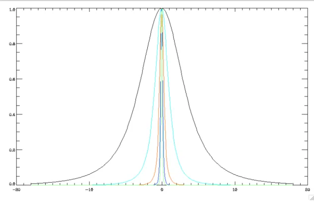
In our LAT realistic simulations, the PSF width depends strongly on the energy, from 6.9˝ at
50 MeV to better than 0.1˝ at 10 GeV and above. Figure 4 shows the normalized profiles of the
Figure 2. Result of the multichannel Poisson denoising algorithm on simulated Fermi data over the energy band 589 MeV - 965 MeV. Top: Simulated intensity skymap. Middle: Simulated noisy skymap. Bottom: denoised skymap. Maps are on a logarithmic scale.
4.2. Monochannel Deconvolution
We first consider the single-channel case. In the literature, several algorithms have been proposed to perform image deconvolution on a cartesian grid. The Richardson-Lucy algorithm is certainly the most famous in astrophysics. In this paper, we propose a regularized Richardson-Lucy algorithm to deconvolve data on the sphere data.
The Richardson-Lucy algorithm originates from a fixed-point equation obtained by maximizing the Poisson likelihood with respect to X while preserving positivity. This entails a multiplicative
Figure 3. Spectrum of a single gamma-ray point source recovered using the multichannel MS-VSTS denoising algorithm. Top: Single gamma-ray source from simulated Fermi data integrated along the energy axis (left: simulated source; middle: noisy source; right: denoised source). Bottom: Spectrum of the center of the point source: intensity as a function of the energy band with 14 energy bands between 50 MeV and 50 GeV (black: true simulated spectrum; cyan: restored spectrum from our denoising algorithm.
update rule, starting at n “ 0 and Xp0q
“ 1 and iterating Xpn`1q “ Xpnqb ´ HTpY c HXpnqq ¯ , (23)
where b (respectively c) represents the element-wise multiplication (respectively division) between two vectors, and HT is the transpose of H whose action on an image consists in convolving it with the time-reversed version of the PSF associated with H. However, it is well-known that owing to the lack of regularization, the Richardson-Lucy algorithm tends to amplify the noise after a few iterations.
We define Rpnqas the residual at iteration n
Rpnq
“ Y ´ HXpnq, (24)
where Rpnq can be written as the sum of its IUWTS detail subband td
ju1ďjďJ and the last
ap-proximation subband aJ, that is,
Rpnq rkrs “ aJrkrs ` J ÿ j“1 djrkrs, @kr. (25)
The wavelet transform provides a means of extracting only the significant structures from the residual at each iteration. With increasing number of iterations, a large part of the residual becomes statistically insignificant. The regularized significant residual is then, for a location kr
s Rpnq rkrs “ aJrkrs ` ÿ pj,krqPM djrkrs , (26)
where M is the multiresolution support defined in a similar way to Eq. (19). The regularized Richardson-Lucy scheme then becomes
Xpn`1q “ P` ´ Xpnq b ´ HT ´ pHXpnq` sRpnq q c HXpnq ¯¯¯ . (27)
Figure 4. Normalized profile of the PSF for different energy bands as a function of the angle in degree. Black: 50 MeV - 82 MeV. Cyan: 220 MeV - 360 MeV. Orange: 960 MeV - 1.6 GeV. Blue: 4.2 GeV - 6.9 GeV. Green: 19 GeV - 31 GeV.
This algorithm is similar to Murtagh et al. (1995), except that the à trous wavelet transform is replaced by the undecimated wavelet transform. In the next subsection, we describe how the same algorithm can be extended to the multi-channel case.
4.3. Multichannel deconvolution
As the PSF is channel-dependent, the convolution observation model is now Y r¨, kts “ HktXr¨, kts ` εr¨, kts
in each channel kt, where Hkt is the (spatial) convolution operator in channel ktwith known PSF. The same recipe as in the monochannel case applies with the notable difference that the spherical 2D-1D MS-VSTS is used instead of its monochannel counterpart. The multichannel multiresolution support M is obtained after thresholding these coefficients.
We now define H to be the multichannel convolution1 operator, which acts on a 2D-1D mul-tichannel spherical data set X by applying Ht to each channel Xr¨, kts independently2. The
regu-larized multichannel Richardson-Lucy scheme is then
Xpn`1q “ P` ´ Xpnq b ´ HT ´ pHXpnq` sRpnq q c HXpnq ¯¯¯ , (28)
where sRpnqis the regularized (significant) residual
s Rpnq rkr, kts “ aJ1,J2rkr, kts ` ÿ pj1,j2,kr,ktqPM wj1,j2rkr, kts . (29) 1
Strictly speaking, this is a slight abuse of terminology since the kernel is not channel-invariant. 2 If X were to be vectorized by stacking the channels in a long column vector, H would be a block-diagonal matrix whose blocks are the circulant matrices Hkt.
4.4. Experiments
The algorithm was applied to the seven energy bands (50 MeV-1.58 GeV) of our simulated Fermi data set. Figures 5 to 8 display the deconvolution results for four energy bands. Figure 9 shows the performance of the multichannel MS-VSTS deconvolution algorithm for a single point source. The deconvolution not only effectively removes the blur and recovers sharply localized point sources, but also allows us to restore all of the spectral information. To get a better visual impression of the performance of the deconvolution algorithm, Figure 10 depicts the result of the algorithm on a single HEALPix face covering the Galactic plane. We find that the deconvolution is remarkably effective : our MS-VSTS multichannel deconvolution algorithm manages to remove a large part of the blur introduced by the PSF.
Software
The software related to this paper, MRS/Poisson, and its full documentation will be included in the next version of ISAP (Interactive Sparse astronomical data Analysis Packages) via the ISAP web site.3
5. Conclusion
This paper extends the MS-VSTS framework to deal with monochannel deconvolution, channel denoising and multichannel deconvolution. Unlike the monochannel MS-VSTS, the multi-channel MS-VSTS fully exploits the information in the 2D-1D data set and allows us to recover the spectral information on the sources. As the PSF strongly depends on the energy, it is very important to have a multichannel method for deconvolution. Multichannel deconvolution using MS-VSTS removes a large part of the PSF blur and significantly improves the sharpness of the spatial localization of point sources.
Acknowledgements. Some of the results in this paper have been derived using the Healpix (Górski et al. 2005) and the MR/S software (Starck et al. 2006). This work was supported by the French National Agency for Research (ANR-08-EMER-009-01) and the European Research Council grant SparseAstro (ERC-228261).
References
Abdo, A. A., Ackermann, M., Ajello, M., et al. 2010, ApJS, 188, 405 Atwood, W. B., Abdo, A. A., Ackermann, M., et al. 2009, ApJ, 697, 1071
Conrad, J., Scargle, J., & Ylinen, T. 2007, in American Institute of Physics Conference Series, Vol. 921, The First GLAST Symposium, ed. S. Ritz, P. Michelson, & C. A. Meegan, 586–587
Donoho, D. 2004, For Most Marge Underdetermined Systems of Linear Equations, the minimal l1-norm solution is
also the sparsest solution, Tech. rep., Department of Statistics of Stanford University Faÿ, G., Delabrouille, J., Kerkyacharyan, G., & Picard, D. 2011, ArXiv e-prints
Górski, K. M., Hivon, E., Banday, A. J., et al. 2005, Astrophysical Journal, 622, 759–771
Movit, S. 2009, in Bulletin of the American Astronomical Society, Vol. 41, American Astronomical Society Meeting Abstracts, 332.06
Murtagh, F., Starck, J.-L., & Bijaoui, A. 1995, Astronomy and Astrophysics, Supplement Series, 112, 179–189 Norris, J. P., Gehrels, N., & Scargle, J. D. 2010, ApJ, 717, 411
Schmitt, J., Starck, J. L., Casandjian, J. M., Fadili, J., & Grenier, I. 2010, Astronomy and Astrophysics, 517 Schmitt, J., Starck, J.-L., Fadili, J., & Digel, S. 2011, in Advances in Machine Learning and Data Mining for
Astronomy, ed. M. Way, J. Scargle, K. Ali, & A. Srivastava (Chapman and Hall) Starck, J., Fadili, J. M., Digel, S., Zhang, B., & Chiang, J. 2009, A&A, 504, 641
Starck, J.-L., Moudden, Y., Abrial, P., & Nguyen, M. 2006, Astronomy and Astrophysics, 446, 1191
Starck, J.-L., Murtagh, F., & Fadili, M. 2010, Sparse Image and Signal Processing (Cambridge University Press) Yamada, I. 2001, in Inherently Parallel Algorithm in Feasibility and Optimization and their Applications (Elsevier),
pp. 473–504
Zhang, B., Fadili, J., & Starck, J.-L. 2008, IEEE Transactions on Image Processing, vol. 11, no. 6, pp. 1093
Figure 5. Result of the multichannel deconvolution algorithm for different energy bands. Top: Simulated (blurred) intensity skymap. Middle: Blurred and noisy skymap. Bottom: Deconvolved skymap. Energy band : 82 MeV - 134 MeV. Maps are on a logarithmic scale.
Figure 6. Result of the multichannel deconvolution algorithm for different energy bands. Top: Simulated (blurred) intensity skymap. Middle: Blurred and noisy skymap. Bottom: Deconvolved skymap. Energy band : 220 MeV - 360 MeV. Maps are on a logarithmic scale.
Figure 7. Result of the multichannel deconvolution algorithm for different energy bands. Top: Simulated (blurred) intensity skymap. Middle: Blurred and noisy skymap. Bottom: Deconvolved skymap. Energy band : 360 MeV - 589 MeV. Maps are on a logarithmic scale.
Figure 8. Result of the multichannel deconvolution algorithm for different energy bands. Top: Simulated (blurred) intensity skymap. Middle: Blurred and noisy skymap. Bottom: Deconvolved skymap. Energy band : 589 MeV - 965 MeV. Maps are on a logarithmic scale.
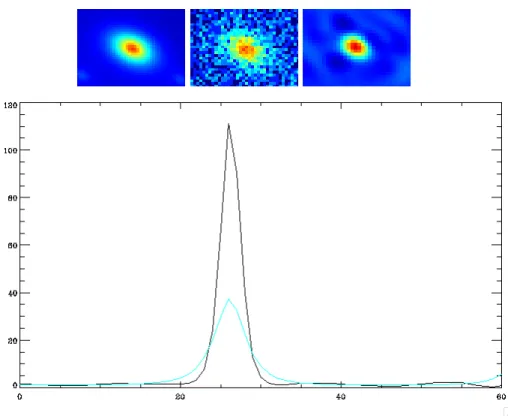
Figure 9. Profile of a single gamma-ray point source recovered using the multichannel MS-VSTS deconvolution algorithm. Top: Single gamma-ray point source on simulated (blurred) Fermi data (energy band: 360 MeV - 589 MeV) (left: simulated blurred source; middle: blurred noisy source; right: deconvolved source). Bottom: Profile of the point source (cyan: simulated spectrum; black: restored spectrum from the deconvolved source.
Figure 10. View on a single HEALPix face. Result of an application of the deconvolution algorithm to the Galactic plane. Top Left: Simulated Fermi Poisson intensity. Top Right: Simulated Fermi noisy data. Bottom: Fermi data deconvolved with multichannel MS-VSTS. Energy band: 360 MeV - 589 MeV. Pictures are on a logarithmic scale.