The LOFAR Two-metre Sky Survey I. Survey description and preliminary data release*

HAL Id: insu-01521308

https://hal-insu.archives-ouvertes.fr/insu-01521308

Submitted on 16 May 2017

HAL is a multi-disciplinary open access

archive for the deposit and dissemination of

sci-entific research documents, whether they are

pub-lished or not. The documents may come from

teaching and research institutions in France or

abroad, or from public or private research centers.

L’archive ouverte pluridisciplinaire HAL, est

destinée au dépôt et à la diffusion de documents

scientifiques de niveau recherche, publiés ou non,

émanant des établissements d’enseignement et de

recherche français ou étrangers, des laboratoires

publics ou privés.

Distributed under a Creative Commons Attribution - NonCommercial - NoDerivatives| 4.0

International License

The LOFAR Two-metre Sky Survey I. Survey

description and preliminary data release*

T. W. Shimwell, H.J.A. Röttgering, P Best, W.L. Williams, J.T Dijkema, F.

de Gasperin, D N Hoang, M. J. Hardcastle, H Heald, A Horneffer, et al.

To cite this version:

T. W. Shimwell, H.J.A. Röttgering, P Best, W.L. Williams, J.T Dijkema, et al.. The LOFAR

Two-metre Sky Survey I. Survey description and preliminary data release*. Astronomy and Astrophysics

- A&A, EDP Sciences, 2017, 598, A104 (22 p.). �10.1051/0004-6361/201629313�. �insu-01521308�

November 10, 2016

The LOFAR Two-metre Sky Survey – I. Survey Description

and Preliminary Data Release

T. W. Shimwell

, H. J. A. Röttgering

, P. N. Best

, W. L. Williams

, T.J. Dijkema

, F. de Gasperin

, M. J. Hardcastle

,

G. H. Heald

, D. N. Hoang

, A. Horneffer

, H. Intema

, E. K. Mahony

, S. Mandal

, A. P. Mechev

, L. Morabito

,

J. B. R. Oonk

, D. Rafferty

, E. Retana-Montenegro

, J. Sabater

, C. Tasse

, R. J. van Weeren

, M. Brüggen

,

G. Brunetti

, K. T. Chy˙zy

, J. E. Conway

, M. Haverkorn

, N. Jackson

, M. J. Jarvis

, J. P. McKean

, G. K.

Miley

, R. Morganti

, G. J. White

, M. W. Wise

, I. M. van Bemmel

, R. Beck

, M. Brienza

, A. Bonafede

,

G. Calistro Rivera

, R. Cassano

, A. O. Clarke

, D. Cseh

, A. Deller

, A. Drabent

, W. van Driel

, D. Engels

,

H. Falcke

, C. Ferrari

, S. Fröhlich

, M. A. Garrett

, J. J. Harwood

, V. Heesen

, M. Hoeft

, C. Horellou

, F. P.

Israel

, A. D. Kapi´nska

, M. Kunert-Bajraszewska

, D. J. McKay

, N. R. Mohan

, E. Orrú

, R. F. Pizzo

, I.

Prandoni

, D. J. Schwarz

, A. Shulevski

, M. Sipior

, D. J. B. Smith

, S. S. Sridhar

, M. Steinmetz

, A. Stroe

, E.

Varenius

, P. P. van der Werf

, J. A. Zensus

, J. T. L. Zwart

(Affiliations can be found after the references)

Accepted —; received —; in original form November 10, 2016

ABSTRACT

The LOFAR Two-metre Sky Survey (LoTSS) is a deep 120-168 MHz imaging survey that will eventually cover the entire Northern sky. Each of the 3170 pointings will be observed for 8 hrs, which, at most declinations, is sufficient to produce ∼500resolution images with a sensitivity of ∼100 µJy/beam and accomplish the main scientific aims of the survey which are to explore the formation and evolution of massive black holes, galaxies, clusters of galaxies and large-scale structure. Due to the compact core and long baselines of LOFAR, the images provide excellent sensitivity to both highly extended and compact emission. For legacy value, the data are archived at high spectral and time resolution to facilitate subarcsecond imaging and spectral line studies. In this paper we provide an overview of the LoTSS. We outline the survey strategy, the observational status, the current calibration techniques, a preliminary data release, and the anticipated scientific impact. The preliminary images that we have released were created using a fully-automated but direction-independent calibration strategy and are significantly more sensitive than those produced by any existing large-area low-frequency survey. In excess of 44,000 sources are detected in the images that have a resolution of 2500, typical noise levels of less than 0.5 mJy/beam, and cover an area of over 350 square degrees in the region of the HETDEX Spring Field (right ascension 10h45m00s to 15h30m00s and declination 45◦0000000to 57◦0000000).

Key words. surveys – catalogs – radio continuum: general – techniques: image processing

1. Introduction

Performing increasingly sensitive surveys is a fundamental en-deavour of astronomy. Over the past 60 years, the depth, fi-delity, and resolution of radio surveys has continuously im-proved. However, new, upgraded and planned instruments are capable of revolutionising this area of research. The International Low-Frequency Array (LOFAR; van Haarlem et al. 2013) is one such instrument. LOFAR offers a transformational increase in radio survey speed compared to existing radio telescopes. It also opens up a poorly explored low-frequency region of the electro-magnetic spectrum. An important goal that has driven the devel-opment of LOFAR since its inception is to conduct wide and deep surveys. The LOFAR Surveys Key Science Project (PI: Röttgering) is conducting a survey with three tiers of observa-tions: Tier-1 is the widest tier and includes low-band antenna (LBA) and high-band antenna (HBA) observations across the

? _{E-mail: shimwell@strw.leidenuniv.nl}

whole 2π steradians of the Northern sky; deeper 2 and Tier-3 observations are focussing on smaller areas with high-quality multi-wavelength datasets.

Here we focus on the ongoing LOFAR HBA 120-168 MHz Tier-1 survey, hereafter referred to as the LOFAR Two-metre Sky Survey (LoTSS). This is the second northern hemisphere survey that will be conducted with the LOFAR HBA and is sig-nificantly deeper than the first, the Multifrequency Snapshot Sky Survey (MSSS; Heald et al. 2015). MSSS was primarily con-ducted as a commissioning project for LOFAR and a testbed for large-scale imaging projects, whereas LoTSS will probe a new parameter space. LoTSS is a long term project but over 2,000 square degrees of the northern sky have already been observed and additional data are continuously being taken.

The main scientific motivations for LoTSS are to explore the formation and evolution of massive black holes, galaxies, clusters of galaxies and large-scale structure. More specifically, the survey was initially designed to detect: 100 radio galaxies at z > 6 (based on the predicted source populations of Wilman et al. 2008); and diffuse radio emission associated with the intra-cluster medium of 100 galaxy clusters at z > 0.6 (Enßlin

& Röttgering 2002 and Cassano et al. 2010); along with up to 3 × 107 other radio sources. In addition, the survey had to meet practical requirements such as high efficiency, manage-able data rates with sufficient time and frequency resolution, a workable data processing strategy, good uv plane coverage with sensitivity to a wide range of angular scales, and a feasible to-tal duration. These criterion resulted in the ambitious observa-tional aims of producing high-fidelity 150 MHz images of the entire Northern sky that have a resolution of ∼ 500 and sensi-tivity of ∼ 100 µJy/beam at most declinations (equivalent to a depth of ∼ 20 µJy/beam at 1.4 GHz for a typical synchrotron radio source of spectral index α ∼ −0.7, where the radio flux density Sν∝ να).

Besides the primary objectives there are many other impor-tant science factors that have further motivated the LoTSS. The survey will significantly increase the known samples of young and old AGN, including giant, dying and relic sources, allow-ing detailed studies of the physics of AGN. It will also de-tect millions of AGN out to the highest redshifts (Wilman et al. 2008), including obscured AGN, radiatively-inefficient AGN, and ‘radio-quiet’ AGN, and thus allow statistical studies of the evolution of the properties of different classes of AGN over cos-mic time (e.g. Best et al. 2014). The sensitive images of the steep spectrum radio emission from local galaxy clusters, and the ex-pected detection of hundreds of galaxy clusters out to moderate redshifts, will transform our knowledge of magnetic fields and particle acceleration mechanisms in clusters (e.g. Cassano et al. 2010). Hundreds of thousands of star-forming galaxies will be detected, primarily at lower redshifts but extending out to z >_{∼ 1.} These will be used to distinguish between various models that describe the correlation between the low frequency radio contin-uum and the far-infrared emission and the variation of this cor-relation with galaxy properties (e.g. Hardcastle et al. 2016 and Smith et al. 2014). They will also trace the cosmic star-formation rate density in a manner unaffected by the biases of dust obscu-ration or source confusion (e.g. Jarvis et al. 2015). The survey images, in combination with other datasets, will be used to mea-sure cosmological parameters, including tests of alternative the-ories of gravity, and using the Integrated Sachs-Wolfe effect to constrain the nature of dark energy (e.g. Raccanelli et al. 2012, Jarvis et al. 2015 and Schwarz et al. 2015). Detailed maps of nearby galaxies will be used for studies of cosmic ray diffusion and magnetic fields. The shortest LOFAR baselines (less than 50 m) allow for degree scale emission to be accurately recovered, and the number of well imaged supernova remnants and HII re-gions will be increased by an order of magnitude to forward stud-ies of the interstellar medium and star formation. Galactic syn-chrotron emission mapping will provide new information about the strength and topology of the large-scale galactic magnetic field (Iacobelli et al. 2013).

In addition, the survey datasets will be used for a range of other projects. The low-frequency polarisation maps will be used by the Magnetism Key Science project to measure the Faraday spectra of sources (Beck et al. 2013). The high spectral reso-lution makes it possible to investigate the physics of the cold, neutral medium in galaxies and its role in galaxy evolution by means of radio recombination lines (e.g. Oonk et al. 2014 and Morabito et al. 2014). The wide area coverage will allow for tight constraints on the population of transient sources and the exploration of new parameter space will open up the possibility of serendipitous discoveries. The eventual exploitation of inter-national baselines will facilitate science that requires subarcsec-ond resolution. For example, it will allow us to access a regime in which AGN and star-forming galaxies can be accurately

distin-guished by morphology (e.g. Muxlow et al. 2005) , and because of the large number of detected sources, we will also be able to discover rare objects such as strongly lensed radio sources which can yield constraints on galaxy evolution (e.g Sonnenfeld et al. 2015) and the distribution of dark matter substructure (see Jack-son 2013 and references within).

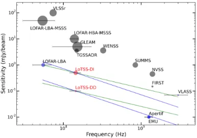
The long integration time on each survey grid pointing that can be afforded due to the wide field of view of the HBA stations, together with the extensive range of baseline lengths in the array, allow the LoTSS to probe a combination of depth, area, resolu-tion and sensitivity to a wide range of angular scales that has not previously been achieved in any wide-area radio survey (see Fig-ure 1). For example, in comparison to other recent low-frequency surveys, such as the TIFR GMRT Sky Survey alternative data release (TGSS; Intema et al. 2016), MSSS (Heald et al. 2015), GaLactic and Extragalactic All-sky MWA (GLEAM; Wayth et al. 2015) and the Very Large Array Low-frequency Sky Survey Redux (VLSSr; Lane et al. 2014), the 120-168 MHz LoTSS will be at least a factor of 50-1000 more sensitive and 5-30 times higher in resolution (see Table 1).

In comparison to higher frequencies the LoTSS will match the high resolution achieved by Faint Images of the Radio Sky at Twenty-Centimeters (FIRST; Becker, White, & Helfand 1995) but over a wider area and, for a typical radio source of spec-tral index α ∼ −0.7, it will be 7 times more sensitive. Simi-larly, the LoTSS will be 20 times more sensitive to typical ra-dio sources than the lower resolution NRAO VLA Sky Survey (NVSS; Condon et al. 1998) and the dense core of LOFAR provides a large improvement in surface brightness sensitivity. There are other large upcoming radio surveys that are mutually complementary with the LoTSS. For example, the LOFAR HBA and LBA sky surveys will be exceptionally sensitive to steep spectrum (α ≤ −1) objects. By comparison, the Evolutionary Map of the Universe (EMU; Norris et al. 2011) and APERture Tile In Focus (Apertif; Röttgering et al. 2011) 1.4 GHz surveys, whilst at lower resolution, aim to reach a depth of ∼ 10 µJy/beam (corresponding to 50 µJy/beam at 150 MHz for α ∼ −0.7) and will offer improved sensitivity to typical or flatter spectrum radio emission. Meanwhile, the 1-3 GHz VLA Sky Survey (VLASS1), will not survey as deeply, but will provide images with 2.500 res-olution to pinpoint the precise location of sources.

In this publication, we describe the LoTSS strategy, and the current calibration and imaging techniques. We also re-lease preliminary 120-168 MHz images and catalogues of over 350 square degrees from right ascension of 10h45m00s to 15h30m00s and declination 45◦0000000 to 57◦0000000 which is in the region of the Hobby-Eberly Telescope Dark Energy Ex-periment (HETDEX) Spring Field (Hill et al. 2008). This field was targeted as it is a large contiguous area at high elevation for LOFAR, whilst having a large overlap with the Sloan Digital Sky Survey (SDSS; York et al. 2000) imaging and spectroscopic data. Importantly, it also paves the way for using HETDEX data to provide emission-line redshifts for the LOFAR sources and prepares for the WEAVE-LOFAR2survey which will measure spectra of more than 106LOFAR-selected sources (Smith 2015). The region was also chosen because HETDEX is a unique sur-vey that is very well matched to the key science questions that the LOFAR surveys aims to address. In particular, the ability to obtain [OII] redshifts up to z ∼ 0.5 is well matched to the LO-FAR goal of tracking the star-formation rate density using ra-dio continuum observations. Furthermore, the main science goal

1 _{https://science.nrao.edu/science/surveys/vlass} 2 _{http://www.ing.iac.es/weave/weavelofar/}

of HETDEX is to obtain emission line redshifts using Lyα at 1.9 < z < 3.5, which is around the peak in the space density of powerful AGN as well as the peak of the star formation rate and the merger rate of galaxies (Jarvis & Rawlings 2000, Rigby et al. 2015, Madau & Dickinson 2014 and Conselice 2014), and will thus help to provide the necessary data for a full census of radio sources over this cosmic epoch. The LOFAR data can help the HETDEX survey to distinguish between low-redshift [OII] and high-redshift Lyα emitters, e.g. using the Bayesian framework set out in Leung et al. (2015).

The greatest challenge we face in reaching the observational aims of the LoTSS is to routinely perform an accurate, ro-bust, and efficient calibration of large datasets to minimise the direction-dependent effects that severely limit the image quality. This complex direction-dependent calibration procedure, which corrects for the varying ionospheric conditions (e.g. Mevius et al. 2016) and errors in the beam models, is crucial to create high-fidelity images at full resolution and sensitivity. Several approaches are being developed to minimise these direction-dependent effects (e.g. Tasse 2014 and Yatawatta 2015), includ-ing the facet calibration procedure (van Weeren et al. 2016a and Williams et al. 2016). This procedure has already been success-fully applied to several fields to produce high-resolution images with high fidelity and a sensitivity approaching the thermal noise (Williams et al. 2016, van Weeren et al. 2016b, Shimwell et al. 2016 and Hardcastle et al. 2016).

A direction-dependent calibration technique will be used to calibrate all LoTSS data in the future to produce images that meet our observational aims, but the exact procedure is still be-ing finalised. Therefore, for this publication, we simply demon-strate that we can achieve these ambitious imaging aims by performing a direction-dependent calibration of a single ran-domly chosen field to produce an 120-168 MHz image with 4.800× 7.900 resolution and 100 µJy/beam sensitivity. However, our large data release consists of preliminary images and cat-alogues that were instead created with a rapid and automated direction-independent calibration of the 63 HBA pointings that cover over 350 square degrees in the region of the HETDEX Spring Field. Although ionospheric and beam effects do hin-der the image fidelity of these preliminary images, we are able to image data from baselines shorter than 12 kλ to produce 2500 resolution images that typically have a noise level of 200-500 µJy/beam away from bright sources. Such sensitive, low-frequency images have not previously been produced over such a wide area and are sufficient to accomplish many of the scien-tific objectives of the survey (see Brienza et al. 2016, Harwood et al. 2016, Heesen et al. 2016, submitted, Mahony et al. 2016, Shulevski et al. 2015a and Shulevski et al. 2015b for examples). The outline of this paper is as follows. In Section 2, we describe the survey strategy including the choice of observing mode, frequency coverage, dwell time, tiling, and the data that are archived. The status of the observing programme for the LoTSS is summarised in Section 3. In Sections 4, 5, 6 and 7 we describe the calibration techniques, imaging procedure, im-age quality and source cataloguing that we have used for this preliminary data release. The data release itself is summarised in Section 8. In Section 9 we provide an example of the im-provement in image fidelity, sensitivity and resolution that will be achieved once direction-dependent calibration has been per-formed on our datasets. Section 10 provides a brief overview of the scientific potential of the LoTSS data before we summarise in Section 11.

Fig. 1. A summary of the sensitivity, frequency and resolution of a se-lection of recent and planned large-area radio surveys (see also Table 1). The size of the markers is proportional to the square root of the sur-vey resolution. Grey, blue and red markers show the ongoing/completed surveys, forthcoming surveys, and the LOFAR HBA surveys respec-tively. The horizontal lines show the frequency coverage for surveys with large fractional bandwidths (> 0.2). The green sloping lines show the sensitivity that is equivalent to that achieved in the LoTSS direction-dependent (DD) calibrated and direction-indirection-dependent (DI) images for typical radio sources with a spectral index ∼ −0.7 . Similarly, the blue sloping lines show the equivalent sensitivity to steep spectrum sources with a spectral index ∼ −1.0.

2. Survey strategy

Prior to routinely undertaking observations for the large-scale LoTSS, the array configuration, integration time, frequency cov-erage, and tiling strategy were chosen. The main aim of the LOFAR HBA survey is to observe the entire Northern sky and achieve a resolution of 500 and a sensitivity of ∼100 µJy/beam at most declinations. In this section we outline the strategy we have adopted to efficiently conduct a survey that can accom-plish this goal which is summarised in Table 2. In choosing our observing setup we bore in mind that, for legacy value, the archived data should be able to facilitate as much science as pos-sible. The archived data should be capable of exploiting the facts that LOFAR has a native spectral resolution suitable for spectral line studies and, while the majority of LOFAR stations are in the Netherlands, at the time the data presented here were taken, there were also international stations in Germany, France, Swe-den and the UK that provide baselines up to 1300 km. The array has been further extended during 2016 to increase the maximum baseline length to 1600 km with three new stations in Poland, and a station in Ireland is currently under construction. These international stations will allow HBA imaging at resolutions of ∼ 0.300. Imaging at the full resolution provided by the interna-tional stations has been shown to be possible for individual tar-gets (e.g. Varenius et al. 2015 with the HBA and Morabito et al. 2016 with the LBA), reaching sensitivities of 150 µJy/beam for the HBA. Accordingly, international stations are present in the LoTSS datasets, although these data are not yet routinely imaged as part of the Survey programme. Such routine imaging will require further work on identification of calibrator sources with significant compact structure, which is currently being un-dertaken by the LBCS project (Moldón et al. 2015 and Jackson et al. 2016, submitted). It will also require further work on the calibration and understanding of ionospheric effects, which is currently under way (e.g. Mevius et al. 2016).

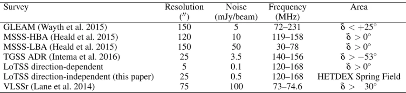
Table 1. A summary of recent large area low-frequency surveys (see also Figure 1). We have attempted to provide a fair comparison of sensitivities and resolutions but we note that both the sensitivity and resolution achieved varies within a given survey.

Survey Resolution Noise Frequency Area

(00) (mJy/beam) (MHz)

GLEAM (Wayth et al. 2015) 150 5 72–231 δ < +25◦ MSSS-HBA (Heald et al. 2015) 120 10 119–158 δ > 0◦ MSSS-LBA (Heald et al. 2015) 150 50 30–78 δ > 0◦ TGSS ADR (Intema et al. 2016) 25 3.5 140–156 δ > −53◦ LoTSS direction-dependent 5 0.1 120–168 δ > 0◦ LoTSS direction-independent (this paper) 25 0.5 120–168 HETDEX Spring Field VLSSr (Lane et al. 2014) 75 100 73–74.6 δ > −30◦

2.1. Observing mode

LOFAR can observe with several different configurations of the HBA tiles, which are described in van Haarlem et al. 2013 and on the observatory’s webpage3. The configurations that affect the core stations are: HBA_ZERO or HBA_ONE, which make use of only one of the two sub-stations in each core station;

HBA_DUAL, which correlates the signal from each sub-station in each core station separately; and HBA_JOINED, where the two sub-stations in each core station act as a single station which results in different beam shapes for different stations. For each configuration the number of tiles used on a remote station can also be selected to be either the inner 24 tiles (to match the core station sub-stations) or the full 48 tiles. At the time of writing, international stations always observe with their full 96 tiles. For the LoTSS, we decided to use HBA_DUAL_INNER, where all stations within the Netherlands operate with 24 tiles and each sub-station in the core stations is correlated separately. This con-figuration was chosen because it does not reduce the number of short baselines or suffer from additional calibration difficulties caused by non-uniform beam shapes. By discarding 24 of the 48 tiles of the remote stations, we reduce the sensitivity but gain a wider field of view.

2.2. Observing bandwidth and integration time

Both the dwell time on each survey pointing and the frequency range allocated, are primarily dictated by the desired sensitiv-ity of ∼100 µJy/beam but this must be coupled with the need for efficient observing and the desire to simplify book-keeping and scheduling. The most efficient HBA observing is performed using the 110-190 MHz band, which has the least radio fre-quency interference (RFI) of the available LOFAR HBA bands. By recording data with 8-bits per sample (at the time of writ-ing a 4-bit mode is bewrit-ing developed but is not yet available for observing) up to 488 195.3 kHz wide sub-bands are available for observing. These sub-bands can be split between multiple station beams, which, for high-sensitivity, must be positioned within the HBA tile beam, which has a full width half maximum (FWHM) of 20◦at 140 MHz (see van Haarlem et al. 2013 for a detailed description of the LOFAR beams). To achieve our target sen-sitivity, the entire 110-190 MHz is not required, as the System Equivalent Flux Density (SEFD) measurements provided by van Haarlem et al. (2013) imply that observing for 8 hrs with 48 MHz of bandwidth within the 110-190 MHz band will allow us to reach our target sensitivity of ∼ 100 µJy/beam. This is also sup-ported by previous observations, for example: van Weeren et al. (2016b) reach 93 µJy/beam noise with 120-181 MHz coverage

3

https://www.astron.nl/radio-observatory/astronomers/technical-information/lofar-technical-information

and 10 hrs of observation; Williams et al. (2016) obtain a sen-sitivity of 110 µJy/beam with 130-169 MHz coverage and 8 hrs of observation; Shimwell et al. (2016) reach 190 µJy/beam with 120-170 MHz coverage and 8 hrs of observation; and Hardcastle et al. (2016) reach 100 µJy/beam sensitivity with 126-173 MHz coverage and 8 hrs integration time.

To increase the efficiency of the observing we use two sta-tion beams simultaneously with 48 MHz of bandwidth allocated to each. The station beams are separated by between four and ten degrees to avoid correlated noise in the regions where the beams overlap, and the tile beam is centred midway between the two station beams to reduce the sensitivity loss. The LOFAR HBA sensitivity varies as a function of frequency due to the gain of the receiving elements (which drops off near the band edges) and the prevalence of RFI. We choose to observe between 120 MHz and 168 MHz to avoid the frequencies within the 110-190 MHz band that have the highest levels of RFI contamination or the poor-est SEFD measurements. This frequency range was also chosen in an attempt to maximise the survey efficiency in terms of the number of sources detected – observing towards the lower end of the HBA band increases the area of the field of view in propor-tion to ν−2and enhances the brightness of sources in proportion to approximately ν−0.7. For simple scheduling, we aim to com-plete the majority of observations with a single integration. To achieve our sensitivity goals we opted to observe each pointing for 8 hrs. Longer tracks were not practical because, similarly to other low-frequency phased arrays, the sensitivity of LOFAR de-creases significantly when observing below 30 degrees in eleva-tion. This is due to, for example, the reduced projected collecting area and the longer line of sight through the ionosphere.

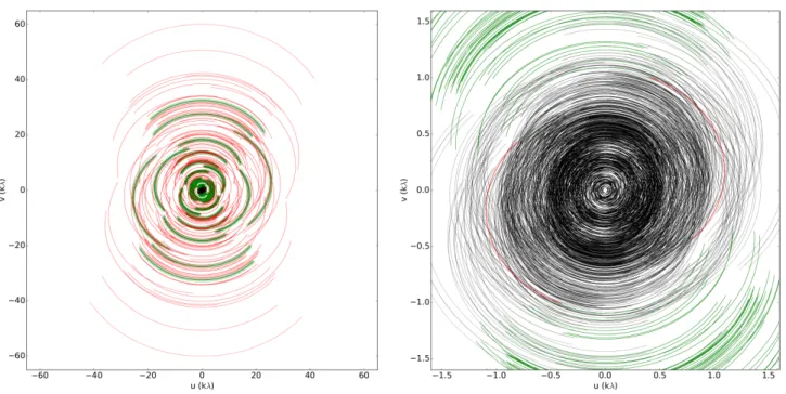
The typical uv-plane coverage of an 8 hr LoTSS observation is shown in Figure 2 (excluding the international stations). The dense core of the array produces a very high density of measure-ments within 2 km which provides excellent surface brightness sensitivity. The most remote stations within the Netherlands pro-vide baselines up to 120 km and allow for ∼ 500resolution imag-ing. The very uneven distribution of points on the uv-plane im-plies that the naturally weighted synthesised beam when imaging with all the Dutch stations of LOFAR has high sidelobes. How-ever, these sidelobes can be reduced significantly by weighting the visibilities with a more uniform weighting scheme such as the Briggs (1995) weighting scheme and using uv-tapers to re-duce the sharpness of cut-offs in the uv-plane coverage.

2.3. Pointing strategy

The FWHM of the LOFAR HBA_DUAL_INNER primary beam is given by

FW HM= 1.02λ

Fig. 2. The monochromatic uv plane coverage of a typical 8 hr 150 MHz LoTSS observation around declination +55◦ excluding the interna-tional stations. On the left is the full uv coverage and on the right we show the dense uv-coverage in the inner region of the uv-plane. Here the monochromatic coverage has been presented for display purposes but the full bandwidth used in each observation is 48 MHz, which corresponds to a fractional bandwidth of ∼1/3, and this provides considerable additional filling of the uv-plane. The uv points are colour coded according to the type of stations that make up each baseline. Those containing only core stations, remote stations, or a combination of the two are shown in black, red, and green respectively.

where λ is the observing wavelength and D is 30.75 m, the di-ameter for theHBA_DUAL_INNERstations (van Haarlem et al. 2013). This implies a station beam FWHM of 4.75◦at 120 MHz, 3.96◦at 144 MHz and 3.40◦at 168 MHz. Nyquist sampling the LoTSS pointings at the highest observed frequency would be required to accurately reconstruct spatial scales that are sim-ilar to the primary beam size (Cornwell 1988) but would re-sult in a large number of pointing centres and is not required to obtain close to uniform sensitivity across the sky. A much coarser sampling is typically used for interferometric radio sur-veys, for example, at the Australia Telescope Compact Array (ATCA4) a separation of FWHM/√3 is recommended and for the Very Large Array (VLA), the NVSS survey Condon et al. (1998) found that a separation of FWHM/√2 would provide nearly uniform sensitivity coverage (the lowest sensitivity be-ing about 90% of the highest sensitivity) and ended up usbe-ing an even coarser spacing of FWHM/1.2. These previous expe-riences indicate that for the highest frequency of the LOFAR HBA survey (168 MHz) the separation between pointing cen-tres should not exceed 2.80◦ (FWHM/1.2). However, for more uniform sensitivity the pointings should be separated by around 2.40◦(FWHM/√2). To give an indication of approximately how many pointings this requires, we find that to hexagonally tile a plane with an area equal to half the sky at 2.80◦separation can be done with 2973 pointings while 2.40◦separation requires 4134 pointings. The final separation we have chosen is a compromise between the time taken to observe the sky and the desired uni-formity. We decided to aim for a separation of ≈2.58◦which samples the sky at our lowest observed frequency close to the Nyquist criterion and approximately samples by FWHM/√2 at the highest frequencies.

4 _{http://www.atnf.csiro.au/computing/software/miriad/}

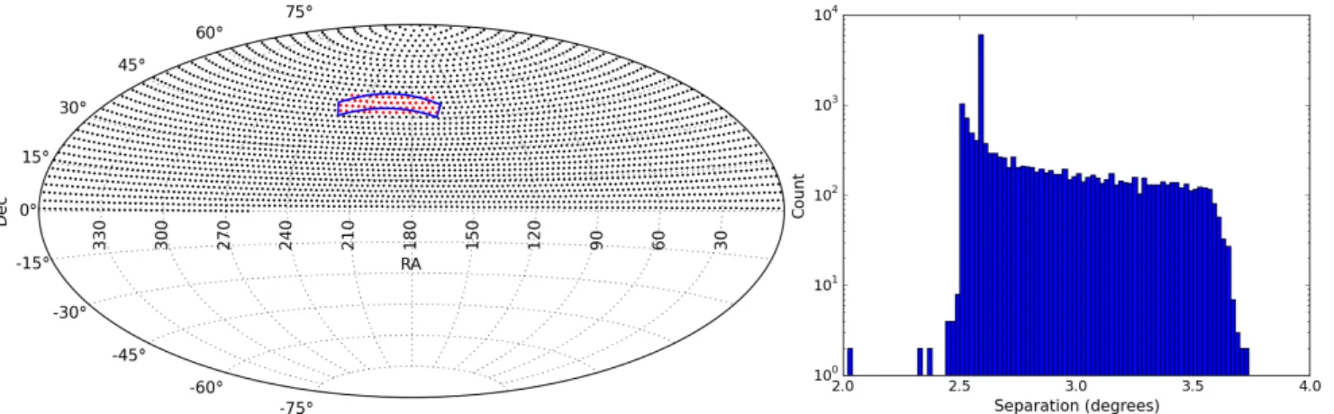
Various tiling strategies have been adopted to perform large area radio surveys but many are based around the efficient hexag-onal close-packed grid structure. For example, the VLA NVSS (Condon et al. 1998) and FIRST (Becker, White, & Helfand 1995) surveys used similar strategies, adopting a hexagonal close-packed grid with a fixed right ascension separation over a certain declination range, but with a declination spacing that varied with approximately 1/cos(dec) to keep a roughly con-stant number of pointing centers per unit area on the sphere. The WENSS survey (Rengelink et al. 1997) used a hexagonal grid with rows of constant declination throughout but altered the right ascension separation of a certain declination range. The VLSS (Cohen et al. 2007) and MSSS (Heald et al. 2015) sur-veys, which have a much larger primary beam than the higher frequency surveys, again used an approximately hexagonal grid pattern to cover the sky but the GLEAM (Wayth et al. 2015) sur-vey, which also has a very large primary beam, used a drift scan technique over declination strips. We have adopted a slightly dif-ferent scheme where our pointing positions are determined using the Saff & Kuijlaars (1997) algorithm which attempts to uni-formly distribute a large number of points over the surface of a sphere. This algorithm produces a spherical spiral distribution of pointings (see Figure 3), where the pointing centres do not lie on rows of constant declination but the structure of adjacent point-ing centres resembles a hexagonal close-packed grid structure.

Using the Saff & Kuijlaars (1997) algorithm to populate the Northern hemisphere with pointings that are typically separated by 2.58◦we have identified 3170 pointing locations which make up the LoTSS grid. The distribution of the separation of pointing positions and the final grid for the LoTSS is shown in Figure 3. We note that 42 of the first pointings to be observed were test observations for the survey and were tiled using a slightly differ-ent scheme which had a similar separation but followed rows of constant declination. Our final survey spherical spiral grid was

rotated so that it best matched up with these early observations. The slight mismatch between the two strategies is apparent in Figure 3.

The density of pointings in the pointing grid is approximately uniform, but it is known that at low declinations the shape of the LOFAR station beam is significantly enlarged (primarily in the north-south direction) and that the sensitivity of the array is reduced. We have not yet precisely accounted for these vari-ations in the structure of our survey grid, but the enlargement of the station beam at lower declination will result in a larger overlap of neighbouring pointings and, while this does not elim-inate the sensitivity variations with declination, it does help to reduce them. Furthermore, we have initiated a series of observa-tions close to zero declination to observationally characterise the expected sensitivity loss.

2.4. Archived datasets

To facilitate both spectral line and international baseline studies, the data are not heavily averaged in either frequency or time be-fore they are archived in the LOFAR Long Term Archive (5). We have opted to store the data at 1 s time resolution and 12.2 kHz frequency resolution (note that some early observations have up to a factor of 4 more averaging). The effects of the time and bandwidth smearing that this averaging causes can be approxi-mated using the equations of Bridle & Schwab (1989). The time averaging of 1 s is such that for international station imaging at 0.500 resolution, time smearing will reduce the peak brightness of sources 1◦away from the pointing centre by 7%. The effects of the 12.2 kHz frequency averaging are approximately equal: at 0.500resolution and 150 MHz the effects of bandwidth smear-ing will reduce the peak brightness of sources 1◦away from the pointing centre by 8%.

Whilst archiving the data at such high time and frequency resolution is crucial to facilitate valuable spectral line and inter-national baseline studies, the downside is that the data volume is very large. The dataset for each pointing is approximately 16 TB, thus the estimated data size for the entire LoTSS is over 50 PB. However, prior to calibrating or imaging the data for the 500 res-olution LoTSS, we can rapidly preprocess the data with an aver-aging of a factor of four in time and four in frequency. This av-eraging can be done because for 500imaging a time resolution of 4 s and a frequency resolution of 48.8 kHz is sufficient to prevent significant smearing within the LOFAR field of view. With this averaging, at a distance of 1.85◦from the pointing centre, which corresponds to the maximum distance at which LoTSS point-ings overlap (see Figure 3), we estimate a 3% peak brightness loss due to time averaging smearing and a 4% peak brightness loss due to bandwidth smearing.

3. Observation status

The LoTSS was initiated on 2014 May 23 in the region of the HETDEX Spring Field and in this publication we present pre-liminary images of the surveyed region between right ascen-sion 10h45m00s to 15h30m00s and declination 45◦0000000 to 57◦0000000 (see Figure 3) that encompass the HETDEX Spring Field. Our observations of this field comprise 63 pointings that were observed between the start of the survey and 2015 October 15. Each pointing was observed for approximately 8 hrs and a calibrator (3C 196 or 3C 295) was observed before and after the observation of the target.

5 _{http://lofar.target.rug.nl}

Table 2. A summary of the LoTSS survey properties. The sensitivity and noise estimates are appropriate for most observations but we note that the sensitivity may be reduced at low declination (see Section 2.3).

Number of pointings 3170 Separation of pointings 2.58◦ Integration time 8 hrs Frequency range 120-168 MHz Array configuration HBA_DUAL_INNER

Angular resolution ∼500 Sensitivity ∼100 µJy/beam Time resolution 1 s∗ Frequency resolution 12.2 kHz∗

∗_{the majority of the earliest ∼ 100 observations were averaged}

to 2 s and 24.4 kHz due to the large data rates.

The 63 LoTSS pointings within the region of the HETDEX Spring Field are only 2% of the total survey. However, by 2016 November we will have gathered data for 350 LoTSS pointings whose coverage spans far beyond the HETDEX region. Our top priority is to complete the survey above declination > 25◦, where the sensitivity of LOFAR is highest: the existing observations correspond to 20% of this region. At the current rate of observa-tions we expect to complete at least this region with the next 5 years.

4. Data reduction

The reduction of the LoTSS data is challenging due to: the large data size; the desire to reduce the data to approximately match the rate at which new observations are performed; the need for almost complete automation; and the complexities involved in calibrating the direction-dependent ionospheric effects and beam model errors. Here we present a preliminary reduction of LoTSS data that was performed with a completely automated direction-independentcalibration and imaging pipeline that we describe in detail in the following subsections. This calibration allows us to create 2500 resolution images with a noise level that is typi-cally in the range from 200 to 500 µJy/beam away from bright sources. However, we emphasise that in the longer term, we will complete a full direction-dependent calibration of these data that will enable us to reach the thermal noise of approximately 100 µJy/beam at a resolution of 500. One such procedure to pro-duce the desired high quality images from similar datasets was recently outlined by van Weeren et al. (2016a) and Williams et al. (2016). At present, this procedure requires too much user inter-action and computational time to be routinely run on the LoTSS datasets but good progress is being made to reduce these require-ments.

4.1. Calibration

The direction-independent calibration procedure we have adopted is similar to that applied in preparation for the direction-dependent facet calibration scheme developed by van Weeren et al. (2016a) and Williams et al. (2016). The difference is that we apply the standard LOFAR station beam model during the imag-ing usimag-ing AWimager (Tasse et al. 2013). For completeness the direction-independent calibration strategy is outlined below.

The data for the target (≈ 8 hrs) and the calibrator (2 × 10 mins) were recorded with 1 second sampling and 64 chan-nels per 0.195 MHz subband. These data were flagged for inter-ference by the observatory using the AOFLAGGER (Offringa,

Fig. 3. The left panel shows the LoTSS pointing grid which follows a spherical spiral structure. The region highlighted in blue is the HETDEX Spring Field. The red points show the LOFAR pointings that are presented in this publication and the black points show the rest of the survey grid. The right panel shows a histogram of the separation of the six nearest neighbours to each of the 3170 pointings in the survey grid excluding the edge pointings close to declination zero. A log scale is used on the y-axis in order to clearly display the full variation of pointing separations. The mean separation of pointings is 2.80◦but the distribution is highly peaked around the median separation of 2.58◦. In total, 65% of pointings have all six nearest neighbours within 2.80◦and 98% have at least four neighbouring pointings within 2.80◦. Note that the panel on the right was created from a grid with a complete spherical spiral structure and ignores the 42 test pointings that were conducted with a slightly different tiling strategy.

van de Gronde, & Roerdink 2012) before being averaged. Only the averaged data products, which have sizes between 3 TB and 16 TB per pointing (depending on the averaging), were stored in the LOFAR archive.

Prior to calibration, the data were downloaded from the LO-FAR Long Term Archive to local computing facilities at a speed of about 30MB/s. At this speed, the retrieval of a 3 TB dataset took ≈1day and a 16 TB dataset took ≈1 week. After the data were retrieved from the archive, we averaged the calibrator data to 4 channels per 0.195 MHz subband and 4 seconds, flagged again for interference (which is identified by AOFLAGGER on the XY and YX polarisations) and removed the international stations from the measurement set if they were included in the observation. Each subband of the calibrator data was then cali-brated using the BLACKBOARD SELFCAL (BBS) software (Pandey et al. 2009) to obtain XX and YY solutions for each time slot and frequency channel, taking into account differen-tial Faraday rotation. In these data the only calibrators observed were 3C 295 and 3C 196, and these were used to calibrate 4 and 59 pointings respectively. The model used for the calibra-tion of 3C 295 uses the flux density scale provided by Scaife & Heald (2012) with the flux density split equally between two point source components separated by 400. The model used for the calibration of 3C 196 is also consistent with the flux density scale described in Scaife & Heald (2012), consisting of a com-pact (< 600maximum separation) group of four narrow gaussian sources (with major axis less than 300) each with a spectral index and curvature term (V. N. Pandey, private communication).

After each subband of the calibrator data has been calibrated, the calibration tables for all 244 subbands are combined into a single table for all 48 MHz of available bandwidth. Using the full-bandwidth calibration table, we smooth the XX and YY am-plitude solutions in time and frequency to provide a frequency-dependent but time-infrequency-dependent amplitude solution for each sta-tion. These solutions are fairly stable with variations of ≈10% over the 18 months that these observations were taken. The ex-act cause of these variations is uncertain but likely includes the stability of the instrument, the elevation of the calibrator, the ob-serving conditions, and the accuracy of the calibrator sky mod-els. In Figure 4 we show example amplitude solutions for all

ob-servations within the HETDEX region for a representative sam-ple of four LOFAR stations, including two core stations and two remote stations.

The full-bandwidth calibration solutions span a sufficiently wide frequency range to allow us to separate the effects of the LOFAR clocks that timestamp the data prior to correlation (each remote station has its own clock and the core stations operate using a single clock) from those of the Total Electron Content (TEC) difference following the scheme described in van Weeren et al. (2016a). These effects can be separated as the clock differ-ence between the stations causes a phase change that is propor-tional to ν, whereas the difference in TEC between the lines of sight of the two stations causes a phase change that is propor-tional to ν−1. Example clock solutions are shown in Figure 5. This shows that the clock values for the core stations are around 0 ns (this is by definition as the plots show the difference between the clocks of each station and the core station CS001HBA0) but the clock values for the remote stations can be ≈ 100 ns. Whilst we find that the clock solutions are generally quite stable, we do see small variations between observations. For example, for the remote stations, we find that there are two discrete groups of clock values (see Figure 5) and that these correspond to Cycle 2 and Cycle 3 observations (where each Cycle corresponds to 6 months of observations) between which the delay calibration was refined by the observatory. Furthermore, there are still vari-ations within the derived clock values for observvari-ations within the same Cycle. This is expected because the remote stations have their own clocks, synchronised with a Global Positioning System (GPS) signal, and are known to drift by within ∼15 ns time-scales during an observation as was demonstrated by van Weeren et al. (2016a).

Similarly to the calibrator field, the target field is averaged to 4 channels per 0.195 MHz subband and 4 seconds, flagged again for interference which is identified on the XY and YX po-larisations and the international baselines are removed from the measurement sets. From almost all our HETDEX observations, the station CS013 is also flagged because until October 2015 the HBA dipoles of this station were rotated at 45◦with respect to the other stations. The time independent clock values and ampli-tude solutions that were derived from the calibrator observations

are then applied to the target data. The transfer of the clock and amplitude values is done at this step, prior to the full averaging of the target data, to reduce decorrelation that the clock offsets may cause on the longest baselines. The target data are then av-eraged by a further factor of 2 in both time and frequency to give a final frequency and time resolution of 2 channels per sub-band and 8 seconds. In Section 2.4 we highlighted the need for less averaging (4 s and 4 channels per subband) when imaging at 500 resolution (see also Williams et al. 2016) but in this pre-liminary data release our imaging is at a much lower resolution of 2500and averaging to 2 channels per subband and 8 seconds causes minimal time or bandwidth smearing in the field of view. In our images of each pointing, the measured peak brightness 2.5◦from the pointing centre should be 98% of their expected value. However, we note that our pointings are mosaiced to pro-duce the final images (see Section 6). Sources in our mosaiced images will all have a reduced peak brightness due to smearing and the reduction will depend upon the position of the source with respect to each of the pointing centres as well the weight-ing of each pointweight-ing in the mosaiced image (see e.g. Prandoni et al. 2000). We have calculated that for sources detected in the central part of our mosaiced region (in pointings with six sur-rounding pointings; see Section 6) the peak brightness loss will be less than 2%, whilst for sources close to the outer edge of the mosaiced region the peak brightness loss remains below 4%.

Due to the wide-field of view and the non-negligible side-lobes of the LOFAR HBA beam it is common that sources in distant sidelobes contribute significant artefacts across the main lobe of the beam. The primary cause of such emission is due to the very bright sources Cygnus A, Cassiopeia A, Virgo A, Tau-rus A and Hercules A. The contamination from these sources is assessed for each pointing by using models of the sources and the LOFAR HBA beam to simulate the response of each of them throughout the observations. These sources are all fur-ther than 35◦from the pointings in the HETDEX Spring Field region, and due to this large separation we are able to efficiently minimise the contamination from them by simply flagging base-lines and time periods where their simulated signal exceeds the observatory-recommended threshold of 5 Jy.

After the bright contaminating sources were removed, the target field data was concatenated into groups of 12 subbands (2.3 MHz) and flagged for interference again with AOFLAG-GER with a strategy that uses the XY and YX polarisations to remove low level interference that was not previously iden-tified. The target data were then phase calibrated with a calibra-tion time interval of 32 seconds against a sky model generated from the VLA Low-Frequency Sky Survey (VLSSr; Lane et al. 2012), Westerbork Northern Sky Survey (WENSS; Rengelink et al. 1997) and the NRAO/VLA Sky Survey (NVSS; Condon et al. 1998) – see The LOFAR Imaging Cookbook6_{or Scheers (2011)}

for details. All VLSS sources within five degrees of the point-ing centre with a flux density greater than 1 Jy are included in the phase calibration catalogue and these sources are matched with WENSS and NVSS sources to include the spectral proper-ties of the sources in the phase calibration catalogue. We note that imperfections in the sky model will result in calibration er-rors and efforts are ongoing to reduce these imperfections by utilising models derived from other surveys such as TGSS (In-tema et al. 2016 and MSSS (Heald et al. 2015). However, even with the sky model we presently use we often find that direction

6

https://www.astron.nl/radio-observatory/lofar/lofar-imaging-cookbook

dependent effects, rather than sky model imperfections, are the primary limitation of the image quality (see Section 4.2).

The control parsets and scripts that have been developed to perform the entire calibration procedure that is described above are executed by the pipeline framework that is now part of the LOFAR software package. Using this pipeline framework makes it simple to efficiently run our completely automated reduction on multiple computers. The pipeline framework handles data tracking, parallel execution, and checks each step is properly completed, which allows for jobs to be resumed. During the pipeline run, various diagnostic plots are produced to assess the quality of the data. For the calibrator observations we ensure that the values derived for the amplitude and clock corrections are good. We also examine the phase solutions from the target to quickly identify observations that suffer from poor ionospheric conditions. After the data are retrieved from the archive, approx-imately 3 days are required to execute this calibration pipeline on 24 threads of one of our compute nodes. Each of our compute nodes have 512 GB RAM and contain four Intel Xeon E5-4620 v2 processors which have eight cores each (16 threads) and run at 2.6 GHz.

The final step is to remove time periods during which the ionospheric conditions are poor. We identify such conditions by locating time periods that have rapid large variations in phase. The phase calibration of the target provides a solution for each station every 32 seconds and, generally, when a nearby station is used for a phase reference, these solutions change smoothly as a function of time. Hence, the difference between these solutions and the same solutions smoothed along the time axis (using a median filter with a window size of 5 samples) is close to 0 ra-dians for short baselines. Therefore, for each station we use the closest station as a reference for the phase solutions and iden-tify periods of rapidly varying phases which are those where the difference between the raw solutions and the smoothed solutions are significant (we set a threshold of 0.29 radians for a 12 sub-band dataset). If, for multiple stations (we use a threshold of 5 stations), we identify the same time period as having a rapidly varying phase the ionospheric conditions are classified as poor and the data are flagged for all stations. We note that that this technique works well if we only use the phase solutions from the core LOFAR stations, where the maximum distance to the near-est station that is used for a phase reference is 1675 m (at this distance the phase solutions do not vary rapidly in normal ob-serving conditions). As the remote stations are isolated, with no other stations nearby, there are often very rapid variations in the phase solutions when the nearest station is used as a phase ref-erence (see e.g. van Weeren et al. 2016a) and poor ionospheric conditions can be more difficult to identify. This procedure to flag time periods with poor ionospheric conditions is demon-strated in Figure 6.

4.2. Imaging

We have somewhat mitigated direction-dependent effects by not utilising the full resolution of the Dutch stations of LOFAR (≈ 500) and only using baselines shorter than 12 kλ (corresponding to ≈ 2500 resolution) when imaging. However, wide-field imag-ing of these direction-independent calibrated LOFAR datasets is still difficult due to the low dynamic range of the images and the large number of bright sources. The high sidelobes of the LOFAR synthesised beam (∼ 12% when imaging our data us-ing the Briggs 1995 weightus-ing scheme and a robust parameter of −0.5) can further hinder this procedure. Furthermore, we use the AWimager (Tasse et al. 2013) to apply the time dependent

120 140 160 180 200 120 130 140 150 160 Frequency (MHz) 120 140 160 180 200

Amplitude calibration factor

120 130 140 150 160

Fig. 4. Amplitude calibration solutions as a function of frequency for the calibrator observations that were used to convert correlator units to Jy for the observations in the HETDEX Spring Field region. The lines show the amplitude solutions for different calibrator observations. The red lines are the solutions when 3C 295 was used as the calibrator and the black lines are when 3C 196 was used. The panels show the am-plitude calibration solutions for two core stations (CS) and two remote stations (RS), from the top left these are: CS003HBA0, CS026HBA0, RS305HBA, RS509HBA. Several calibrator observations show small frequency ranges where bad data results in sharp changes in the ampli-tude solutions. 80 60 40 20 0 20 40 60 80 0 100 200 300 400 500 600 Time (s) 80 60 40 20 0 20 40 60 80 Clock (ns) 0 100 200 300 400 500 600

Fig. 5. Clock offsets as a function of time for the calibrator observations that were used to calibrate observations in the HETDEX Spring Field region. The lines show the clock offsets for different calibration obser-vations. The red lines are the clock solutions when 3C 295 was used as the calibrator and the black lines are when 3C 196 was used. The panels show the clock offsets for two core stations (CS) and two remote stations (RS), from the top left these are: CS003HBA0, CS026HBA0, RS305HBA, RS509HBA. There are several discontinuities in the de-rived clock values which are due to difficulties in converging on the precise clock solution (see van Weeren et al. 2016a), but only the me-dian clock solutions are applied for calibration of the target field.

LOFAR station beam model in the imaging procedure to out-put both primary-beam corrected and uncorrected images, but with this imager we were unable to image all 48 MHz of band-width with a single wide-bandCLEANdue to the large amount of data (∼250 GB of data per pointing), and at the time of

writ-Fig. 6. The phase solutions for station CS401HBA1 using station CS032HBA1 as a phase reference for a LoTSS dataset are shown in blue (CS032HBA1 is the closest station to CS401HBA1 at a distance of 584 m). The red points show the time periods where the phase solutions indicate poor ionospheric conditions (see Section 4.1) and these time periods are subsequently flagged.

ing, multi-frequency deconvolution was not supported. Such a wide-band deconvolution would be preferable as the synthesised beam sidelobes would decrease and it would be easier to iden-tify andCLEANfaint sources. Instead, we image 36 subbands to-gether and create seven images with frequencies approximately evenly spaced across the 120-168 MHz bandwidth (the highest frequency of these seven images consists of ≈28 subbands rather than 36). To efficientlyCLEANthe faint sources in the presence of large artefacts around bright sources we perform an automated multi-thresholdCLEANwhere we progressively removeCLEAN

boxes around bright sources to allow for the faint sources to be properly deconvolved, as described in detail below. Throughout this imaging procedure we weight the visibilities with a robust parameter equal to −0.5 and image an area of 6.5◦× 6.5◦to en-sure that bright sources far down the beam are deconvolved.

We initially CLEAN our Stokes I image to a threshold of 20 mJy/beam without using a CLEAN mask. The PyBDSM

source finding software (Mohan & Rafferty 2015) is then run on the resulting deconvolved apparent brightness image that has an approximately uniform noise across the imaged area, but due to the limited dynamic range there are regions of increased noise around bright sources. This is used to create aCLEANmask that contains islands that tightly encompass all sources detected in the image but not artefacts around bright sources or source side-lobes, and a noise map that accurately describes the local noise at each position in the image. To approximatelyCLEANthe im-age to the local noise at each position, we firstCLEANthe entire image using theCLEANmask and a threshold that is either the largest noise measurement on the PyBDSM generated noise map or 20 mJy/beam (whichever is less). After this deeperCLEANing of the entire field, the brightest sources are essentially fully de-convolved because the local noise is higher in those regions, but the fainter sources are not. Therefore, all pixels where the noise map value exceeds a given threshold are removed from theCLEANmask and the deconvolution is continued to a lower noise level. To properlyCLEANthe faintest sources to the local noise we repeat this procedure three times. This progressively removes the bright sources where the local noise is higher from theCLEANmask and lowers theCLEANthreshold until only the

faintest sources are left in the CLEANmask and the threshold reaches approximately the median value of the noise map. In a few cases, where the images contained very bright sources, we manually tweaked the imagingCLEANthresholds to improve the deconvolution.

To create full bandwidth images, the seven different images across the band were stacked in the image plane. To do this, for each pointing, the images are convolved with a Gaussian inten-sity distribution to give the seven different images across the band the same resolution. The seven images are then stacked together by taking a weighted average of the images where the weight is 1/σ2_{and the noise, σ , is measured from the image by}

fitting a Gaussian probability distribution to pixel values from the non primary beam corrected image and discarding outlying values. Due to the varying amounts of data that are flagged for different pointings, as well as the occasional subbands missing due to telescope errors, the individual pointings consist of vary-ing proportions of different frequency components. Therefore the average weighted frequency of the seven stacked images is naturally slightly different for each pointing, with the average being 149 MHz and the standard deviation 1.5 MHz. Whilst the weighting of the image stacking could be adjusted to give the same weighted average frequency, this would still not ensure that all images have precisely the same frequency coverage.

It is desirable to provide images with a uniform resolution. However, the missing subbands, the data flagged, the observation duration, and the target position will all result in variations in the synthesized beam between observations. We find that our images typically have a synthesised beam major axis FWHM of approx-imately 20.200with a range from 17.800to 24.800, apart from two outlier fields, P2 and P8, which have synthesised beams that ex-ceed 3000. The large synthesised beams are because over 80% of these datasets (which were observed simultaneously) were flagged due to poor ionospheric conditions that were identified by the flagging procedure outlined in Section 4.1. Therefore, we exclude these two fields from further analysis. To make the im-ages uniform in resolution we convolve the remaining 61 imim-ages with a Gaussian of appropriate size to make the beam of each image 25 × 2500.

We note that these LOFAR images could be used to obtain a model of the sky that is higher resolution and more sensi-tive than that used in the initial phase calibration, and that this model could be used to self calibrate the LOFAR datasets. How-ever, this procedure was not followed because self-calibration is time consuming and, while there is a dependance on the qual-ity of the initial sky model in the target region, in most cases it was not found to significantly improve the image quality when imaging at 2500 resolution. This lack of a significant improve-ment in image quality is probably due to direction-dependent effects, rather than imperfections in the sky models that are used for the direction-independent phase calibration, dominating the calibration errors and limiting the image fidelity. In addition, the images could have been used to identify the sources that pro-duced the largest artefacts (such as 3C 295), that could then be removed by constructing good models for the sources and using the peeling technique (see Mahony et al. (2016) for an example of peeling a bright source in LOFAR direction-dependent cal-ibrated images). This operation was not performed due to the large number of sources that would require peeling and the com-putational expense associated with this.

5. Image quality

The 2500resolution images produced from our datasets form

the most sensitive wide-area low-frequency survey yet produced (see Figure 1). The quality of images varies significantly be-tween pointings due to the presence of bright sources in the field and the quality of the input sky model, but it is predominantly dictated by the position- and time-varying ionospheric condi-tions that cannot be corrected by a direction-independent cal-ibration. This prevents accurate high-resolution imaging, as the ionosphere introduces phase errors which cause position changes that are non-negligible in size compared to the synthesised beam. Even though we have only used baselines shorter than 12 kλ when imaging, the uncorrected ionospheric phase errors cause a noticeable blurring of sources, which reduces their peak bright-ness, alters their position and increases the image noise. Further-more, the quality of all our images is significantly hindered by imperfections in the LOFAR beam model which result in large direction-dependent amplitude (i.e. flux density and spectral in-dex) variations as a function of time. The magnitude of all the quality variations amongst images will be reduced substantially once direction-dependent calibration is fully implemented. How-ever, it is likely that poor ionospheric conditions will mean that a large number of directions will be required to properly cali-brate an affected dataset. It may even be the case that, for some pointings, the ionosphere is so spatially variable that there is in-sufficient flux density within each isoplanatic patch to allow the calibration of all directions. Alternatively, it could be that the number of directions becomes so large that the number of de-grees of freedom required for calibration approaches or exceeds the number of independent measurements of visibilities. Point-ings where the ionospheric conditions prohibit a full direction-dependent calibration must be re-observed.

In the following subsections, we use LOFAR source cata-logues for each pointing (created using PyBDSM) to first iden-tify observations conducted in poor ionospheric conditions and exclude these from future analyses before we assess the quality of each of our remaining images by measuring the astrometry of compact objects, the flux density accuracy, and the sensitivity.

5.1. Identifying poor ionospheric conditions

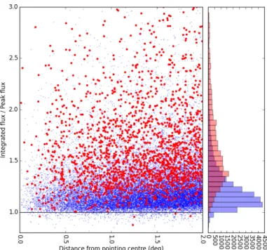
An effective proxy for the ionospheric-induced blurring of sources during LOFAR observations is the ratio of the measured integrated flux density to the peak brightness. This is because the blurring substantially reduces the peak brightness while (except in very poor conditions) the integrated flux density is nearly pre-served. Therefore, quantifying this ratio for each pointing allows us to identify and remove the observations that were conducted in the poorest ionospheric conditions. This procedure is simpli-fied if just compact and isolated sources are used: for compact sources we expect the peak brightness and integrated flux den-sity to be comparable and only selecting isolated sources reduces the probability of mismatched sources or artefacts in the cata-logue. To create such a sample of sources for each pointing, we match the LOFAR catalogue with the FIRST catalogue which is used because it has a high resolution (≈ 500) and helps identify compact sources. The cross matching is performed by simply matching all LOFAR and FIRST sources that are within 1000. Entries are removed from this cross matched catalogue if they are: within 3000of another LOFAR detected source; further than 2◦from the LOFAR pointing centre; have multiple matches; or have sizes greater than 1000 in the FIRST catalogue or greater than 3000in the LOFAR image.

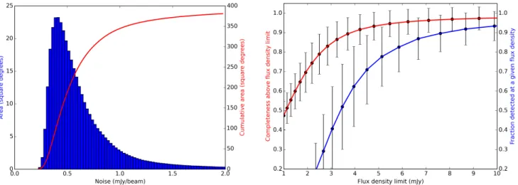
The integrated LOFAR flux density divided by the peak LO-FAR brightness for all objects in our cross matched catalogues is shown in Figure 7. We find that the typical median value of this

Fig. 7. The ratio of the integrated flux density to peak brightness for compact sources in all 54 LOFAR pointings. The seven pointings iden-tified as having particularly poor ionospheric conditions are shown in red and the remaining 54 pointings are shown in blue. The histogram of the red points has been multiplied by a factor of 10 for display purposes.

ratio of compact sources for a pointing is 1.2 but for the 61 point-ings we are analysing it varies from 1.1 to 2.0. There are seven pointings (P6, P164+55, P21, P225+47, P206+50, P221+47 and P33) that we identified as having particularly high integrated flux density to peak brightness ratios (with a median exceeding 1.35) indicating substantial ionospheric blurring. These point-ings are excluded from the remainder of this study, which leaves 54 pointings for further analysis.

5.2. Astrometric uncertainties

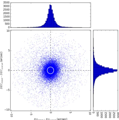
The astrometry of our images is set by our phase calibration, in which we use a model created from the VLSS, WENSS and NVSS surveys (see Section 4.1). These surveys are at lower res-olutions than ours and inaccuracies in the model will not be uncommon. For example, there will be double sources that are unresolved in the lower-resolution model but resolved in our higher-resolution datasets and there will be complex extended emission that is poorly characterised in the model. These imper-fections in the phase calibration catalogue will result in a sys-tematic error in the position of our sources and this will vary between pointings. Furthermore the final astrometric accuracy of our images can also be affected by inaccuracies in the beam model and the ionospheric conditions during the observation. In our images we have not attempted to correct the astrometry for direction dependent calibration effects but we are able to correct systematic position offsets.

To examine the astrometry of our images and correct the systematic astrometric offset for each pointing, we again cross match catalogues of sources from each LOFAR pointing with the FIRST catalogue. The FIRST catalogue was used as it has systematic position errors of less than 0.100 from the absolute radio reference frame, which was derived from high resolution calibrator observations (White et al. 1997). The cross-matching is performed using exactly the same procedure as was described

in Section 5.1. Thus, the final cross matched catalogue contains only compact and isolated sources and this alleviates the issue of possible source brightness distribution changes between the 150 MHz LOFAR and 1.4 GHz FIRST measurements.

The final cross-matched catalogue was used to correct the systematic position offset within each LOFAR pointing. This was done by using the median right ascension and declination offsets (∆RA and ∆Dec) to align the LOFAR source positions with those measured in FIRST. During this process we progres-sively filtered out sources with offsets more than three median absolute deviations (MAD) from the median offset until the me-dian offset converged. The calculated offsets, which range from −3 to 600 in RA and −6 to 300 in DEC, were then applied by altering the headers of the LOFAR image files.

After the correction of the systematic position offset, the LOFAR catalogues were remade and again cross matched with FIRST using the same criteria. It is apparent from this cross matching that the quality of the direction-independent calibra-tion of the LOFAR datasets still varies significantly, which is indicated by variations in both the number of LOFAR sources matched with FIRST sources after filtering out all sources that are not compact and isolated, and the standard deviation of the position offsets. Whilst these variations (e.g. a high standard deviation of the cross-matched source offsets or a low number of cross-matched sources) could be used to further identify ob-servations conducted during poor ionospheric conditions where direction-dependent position offsets are large, we do not use them here. The final astrometric accuracy of the images we have produced through our direction-independent calibration pipeline is displayed in Figure 8. We find that the standard deviation of the offsets, without filtering outliers, is 1.6500in RA and 1.7000in declination which is less than 10% of the synthesised beam size and smaller than the image pixels. By comparison, the TGSS al-ternative data release, which is at a similar resolution to our LO-FAR images but has direction-dependent ionospheric corrections applied, has a standard deviation of 1.5500in the offsets between their measured source positions and those recorded in a VLBA calibrator catalogue (see Figure 13 of Intema et al. 2016). The LOFAR MSSS verification field, which is at a lower resolution of 10800and without a correction for direction dependent effects, has slightly larger offsets of 2.9200in RA and 2.4500in DEC from the NVSS source positions (Heald et al. 2015).

5.3. Flux density uncertainties

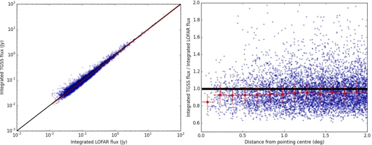
For amplitude calibration, we used models of 3C 196 and 3C 295 to calibrate 94% and 6% of the pointings respectively. The models for both calibrators are on the same flux density scale as the amplitude calibration models that were presented in Scaife & Heald (2012). These models, even in the presence of the known imperfections in the LOFAR HBA beam model, should allow us to obtain flux density accuracies within 10% (see e.g. Heald et al. 2015 and Mahony et al. 2016). However, as we have not corrected for ionospheric phase errors, we expect that our flux measurements may be reduced due to a blurring of the sources, where the peak brightness will be affected significantly more than the integrated flux density as was quantified in Section 5.1. To assess the overall errors on our 150 MHz LOFAR inte-grated flux density and peak brightness measurements, we com-pared with the 7C and TGSS alternative data release measure-ments. After the astrometric correction of our images (see Sec-tion 5.2), we matched our LOFAR sources to these catalogues using the procedure that is outlined in Section 5.1, but as we are not matching with the FIRST catalogue here we did not