HAL Id: hal-00750243
https://hal.inria.fr/hal-00750243
Submitted on 9 Nov 2012
HAL is a multi-disciplinary open access
archive for the deposit and dissemination of sci-entific research documents, whether they are pub-lished or not. The documents may come from teaching and research institutions in France or abroad, or from public or private research centers.
L’archive ouverte pluridisciplinaire HAL, est destinée au dépôt et à la diffusion de documents scientifiques de niveau recherche, publiés ou non, émanant des établissements d’enseignement et de recherche français ou étrangers, des laboratoires publics ou privés.
The ”Back and Forth Nudging” algorithm for
oceanographic data assimilation
Didier Auroux, Jacques Blum
To cite this version:
Didier Auroux, Jacques Blum. The ”Back and Forth Nudging” algorithm for oceanographic data assimilation. 5th WMO Symposium on data assimilation, 2009, Melbourne, Australia. �hal-00750243�
The “Back and Forth Nudging” algorithm for oceanographic data
assimilation
Didier Auroux1 and Jacques Blum1
1
University of Nice Sophia Antipolis, France
1. Introduction
In this paper, we generalize the so-called “nudging” algorithm in order to identify the initial condition of a dynamical system from experimental observations. The standard nudging algorithm consists in adding to the state equations of a dynamical system a feedback term, which is proportional to the difference between the observation and its equivalent quantity computed by the resolution of the state equations.
The Back and Forth Nudging algorithm consists in solving first the forward nudging equation and then a backward equation, where the feedback term which is added to the state equations has an opposite sign to the one introduced in the forward equation. The initial state of this backward resolution is the final state obtained by the standard nudging method. After resolution of this backward equation, one obtains an estimate of the initial state of the system. We iteratively repeat these forward and backward resolutions (with the feedback terms) until convergence of the algorithm. This algorithm is presented in section 2. Then, we present in section 3 a way to choose the forward and backward nudging matrices in order to have well-posed problems, and to obtain the convergence of the algorithm. Then we report in section 4 the results of numerical experiments on several oceanographic models, including comparison and hybridization with the 4D-VAR algorithm. Finally, some conclusions are given in section 5.
2. Back and Forth Nudging (BFN) algorithm
In order to simplify the notations, we assume that the model equations have been discretized in space by a finite difference, finite element, or spectral discretization method. The time continuous model satisfies dynamical equations of the form:
F(X), 0 t T, dt dX < < = (1)
with an initial condition . In this equation, represents all the linear or nonlinear operators of the model equation, including the spatial differential operators. We will denote by 0 ) 0 ( x X = F
H the observation operator, allowing us to compare the
observations with the corresponding , deduced from the state vector . We do not particularly assume
obs
X H(X(t))
) (t
X H to be a linear operator.
If we apply nudging to the model (1), we obtain
F(X) K
(
X H(X))
, 0 t T, dt dX obs − < < + = (2)with the same initial condition, and where K is the nudging (or gain) matrix. Note that it may also be a nudging scalar coefficient in some simple cases. The model then
appears as a weak constraint, and the nudging term forces the state variables to fit as well as possible to the observations. In the linear case (where F is a matrix, and
H is a linear operator), the forward nudging method is nothing else than the
Luenberger observer (Luenberger, 1966), also called asymptotic observer, where the matrix K can be chosen so that the error goes to zero when time goes to infinity. Unfortunately, in most geophysical applications, the assimilation period is not long enough to have the nudging method giving good results. Then, one can apply the nudging technique to the model, but backwards in time, in order to come back to the initial state.
The back and forth nudging algorithm, see e.g. (Auroux et al., 2008), consists of first solving the forward nudging equation and then the backward nudging equation (i.e. the model equation backwards in time, with a nudging feedback to the observations). The initial condition of the backward integration is the final state obtained after integration of the forward nudging equation. At the end of this process, one obtains an estimate of the initial state of the system. We repeat these forward and backward integrations (with the feedback terms) until convergence of the algorithm:
(
)
(
)
⎪ ⎪ ⎩ ⎪⎪ ⎨ ⎧ = > > − − = = < < − + = ≥ − ), ( ) ( ~ , 0 , ) ~ ( ' ) ~ ( ~ ), 0 ( ~ ) 0 ( , 0 , ) ( ) ( 1 1 T X T X t T X H X K X F dt X d X X T t X H X K X F dt dX k k k k obs k k k k k obs k k (3)with the notation 0(0) 0 ~
x
X = . Note that this algorithm can be compared with the 4D-VAR algorithm (Le Dimet et al, 1986), which also consists in a sequence of forward and backward resolutions. But in our algorithm, it is useless to linearize (or differentiate) the system and the backward system is not the adjoint equation but the model equation, with an extra feedback term that stabilizes the ill-posed backward resolution.
3. Choice of the nudging matrices and interpretation
3.1. Variational interpretation of the nudging
The standard nudging method has been widely studied in the past decades (see e.g. Bao et al (1997)). Thus, there are several ways to choose the nudging matrix K in the forward part of the algorithm. One can for example consider the optimal nudging matrix , as discussed in (Vidard et al, 2003). In such an approach, a variational data assimilation scheme is used in a parameter estimation mode to determine the optimal nudging coefficients. This choice theoretically provides the best results for the forward part of the BFN scheme, but the computation of the optimal gain matrix is costly.
opt
K
When , the forward nudging problem (2) simply becomes the direct model (1). On the other hand, setting
0 =
K
+∞ =
K forces the state variables to be equal to the observations at discrete times, as is done in Talagrand (1981). These two choices have the common drawback of considering only one of the two sources of information (model and data).
Let us assume that we know the statistics of errors on observations, and denote by
data assimilation, either variational or sequential. Usually, it is impossible to know the exact statistics of errors, and thus only an approximation of R is available, assumed to be symmetric positive definite.
We assume here the direct model to be linear (or linearized). We consider a temporal discretization of the forward nudging problem (2), using for example an implicit scheme. If we denote by n
X the solution at time and tn n+1
X the solution at time , and , then equation (2) is equivalent to the following optimization problem: 1 + n t n n t t t= − Δ +1 X + = ⎢⎣⎡ X −Xn X −Xn − Δt FX X + Δt R− Xobs −HX Xobs −HX ⎥⎦⎤ X n ), ( 2 , 2 , 2 1 min arg 1 1 (4) if F is symmetric and if the nudging matrix is set to be K =HTR−1. The first two terms correspond exactly to the energy of the discretized direct model, and the last term is the observation part of the variational cost function. This variational principle shows that at each time step, the nudging state is a compromise between minimizing the energy of the system and the distance to the observations.
As a consequence, there is no need to consider an additional term ensuring an initial condition close to the background state like in variational algorithms, neither for stabilizing or regularizing the problem, nor from a physical point of view. One can simply initialize the BFN scheme with the background state, without any information on its statistics of errors.
3.2. Pole assignment method and backward nudging matrix
The goal of the backward nudging term is both to have a backward data assimilation system and to stabilize the integration of the backward system, as this system is usually ill posed. The choice of the backward nudging matrix is then imposed by this stability condition.
If we consider a linearized situation, in which the system and observation operators (F and H , respectively) are linear, and if we make the change of time variable
, then the backward equation can be rewritten as t T t'= −
(
)
, 0 ' . ' ' FX K X HX t T dt dX obs − < < − = − (5)Then, the matrix to be stabilized is −F−K'H , i.e. the eigenvalues of this matrix should have negative real parts. The pole assignment result (see e.g. (Trélat, 2005)) claims that if the system is observable, then there exists at least one matrix such that ' K H K F − '
− is a Hurwitz matrix, i.e. all its eigenvalues are in the negative half-plane. However, such a matrix may be hard to compute, as it usually requires the resolution of a Riccati equation.
4. Numerical experiments
4.1. Numerical choice of the nudging matrices
All numerical experiments have been performed with an easy-to-implement nudging matrix: K =kHTR−1, where is a positive scalar gain, and k R is the covariance
matrix of observation errors. This choice does not require a costly numerical integration of a parameter estimation problem for the determination of the optimal coefficients. Choosing K =HTL, where is a square matrix in the observation space, has another interesting property: if the observations are not located at a model grid point, or are a function of the model state vector, i.e. if the observation operator
L
H involves interpolation/extrapolation or some change of variables, then the
nudging matrix K will contain the adjoint operations, i.e. some interpolation/extrapolation back to the model grid points, or the inverse change of variable.
As in the forward part of the algorithm, for simplicity reasons we make the following choice for the backward nudging matrix: . The only parameters of the BFN algorithm are then the coefficients and . In the forward mode, is usually chosen such that the nudging term remains small in comparison with the other terms in the model equation. The coefficient is usually chosen to be the smallest coefficient that makes the numerical backward integration stable.
1 ' − =k H R K T k k' k >0 ' k 4.2. Experimental approach
The experimental approach consists of performing twin experiments with simulated data. First, a reference experiment is run and the corresponding data are extracted. From now on this reference trajectory will be called the exact solution. Experimental data are supposed to be obtained every grid-points of the model, and every time steps. The simulated data are then optionally noised with a Gaussian white noise distribution, and provided as observations to the assimilation scheme.
x
n nt
The first guess of the assimilation experiments is chosen to be either a constant field or the reference model state some time before the beginning of the assimilation period. Finally, the results of the assimilation process are compared with the exact solution.
4.3. Shallow water model
The shallow water model (or Saint-Venant's equations) is a basic model, representing quite well the temporal evolution of geophysical flows. This model is usually considered for simple numerical experiments in oceanography, meteorology or hydrology. The shallow water equations are a set of three equations, describing the evolution of a two-dimensional horizontal flow. These equations are derived from a vertical integration of the three-dimensional fields, assuming the hydrostatic approximation, i.e. neglecting the vertical acceleration. There are several ways to write the shallow water equations, considering either the geopotential or height or pressure variables. We consider here the following configuration:
⎪ ⎪ ⎪ ⎩ ⎪ ⎪ ⎪ ⎨ ⎧ = ∂ + ∂ + ∂ Δ + − = ∂ + + + ∂ Δ + − = ∂ + + − ∂ , 0 ) ( ) ( , ) ( , ) ( 0 0 hv hu h v rv h B u f v u ru h B v f u y x t y t x t ν ρ τ ς ν ρ τ ς (6)
where ς =∂xv−∂yu is the relative vorticity, ( ) 2 1 2 2 * v u h g B= + + is the Bernoulli potential, g* is the reduced gravity, f is the Coriolis parameter (in the β-plane approximation), ρ0 is the water density, r is the friction coefficient, and ν is the viscosity (or dissipation) coefficient. The unknowns are and the horizontal components of the velocity, and the geopotential height. Finally,
u v
h τ is the forcing
term of the model (e.g. the wind stress) (Durbiano, 2001).
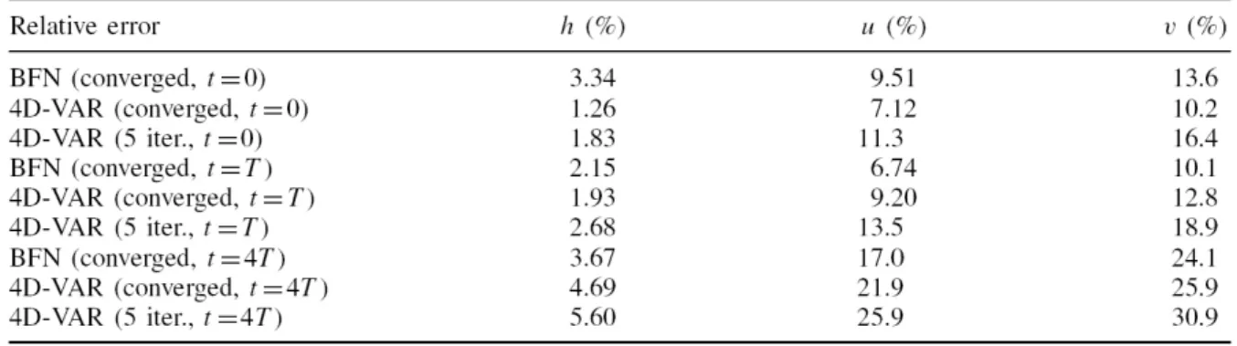
In the following experiments (see (Auroux, 2009) for all numerical results), the observations are available every 5 gridpoints and 24 time steps. The assimilation period lasts 720 time steps, corresponding to 15 days, and the forecast period ends 2880 time steps (or 2 months) after the initial time. As shown in Table 1, the BFN converges in 5 iterations, and we compared it with the 4D-VAR, either at convergence (16 iterations), or stopped after a similar time computation (5 iterations). Several conclusions can be drawn from this table. First the BFN is more efficient than the 4D-VAR in the same time (5 iterations of each). Then, if we compare the results when both algorithms have achieved convergence, the initial condition identified by the 4D-VAR is closer to the true initial state, but the BFN algorithm provides a better solution between time T and 4T, which is a keypoint for the quality of predictions.
Table 1 – Relative error of the forecast solutions corresponding to the BFN (5 iterations, converged), 4D-VAR (16 iterations, converged) and 4D-VAR (5 iterations) identified initial conditions, for the three variables, at various times: initial time, end of the assimilation period, and end of the prediction period.
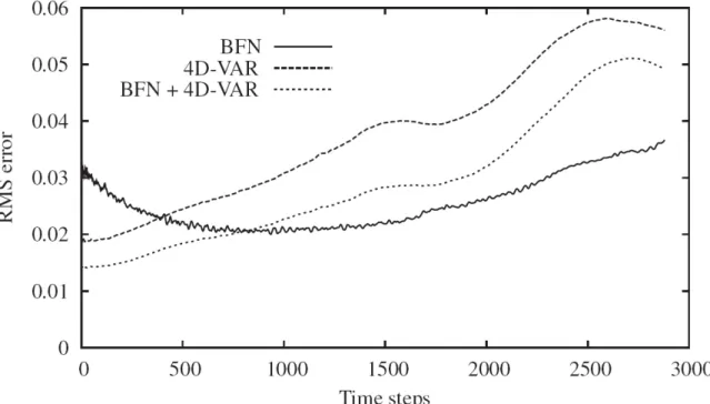
Figure 1 shows a comparison between the BFN and 4D-VAR algorithms, and also a hybrid scheme. As the BFN provides at each iteration a new estimation of the initial condition, it is very easy to hybridize it with another data assimilation method, e.g. the 4D-VAR. We compare in Figure 1 the evolution of the identified trajectories by the BFN and 4D-VAR algorithms (stopped after 5 iterations only), and also the BFN+4D-VAR hybrid scheme in the same computation time. We compare then 5 iterations of BFN, 5 iterations of VAR, and 2 iterations of BFN followed by 3 iterations of 4D-VAR. We can see that during the assimilation period, the best solution is provided by the hybrid algorithm. Note that it would have been improved a little bit by the 4D-VAR at convergence, but we stop all algorithms after 5 iterations here. But during the forecast period, it is still provided by the BFN algorithm, except at the beginning. The results are comparable for u and v, except that the BFN gives a better solution a little earlier. In all the experiments performed, with several levels of noise and different background states, the hybrid method was the best during the assimilation period, and sometimes it was also the best at the beginning of the prediction period, but in most cases, the BFN solution is the best at the end. We can deduce from these
results that a very cheap and simple way to largely improve the 4D-VAR algorithm is to perform very few (2 or 3) iterations of BFN before starting the 4D-VAR minimization process.
Fig. 1 – Relative difference between the true solution and the forecast trajectory corresponding to the BFN, 4D-VAR and BFN-preprocessed 4D-VAR identified initial conditions, after 5 iterations, versus time, for the height variable in the case of noisy observations.
4.4. Quasi-geostrophic ocean model
We have also considered a layered quasi-geostrophic ocean model. This model arises from the primitive equations (conservation laws of mass, momentum, temperature and salinity), assuming first that the rotational effect (Coriolis force) is much stronger than the inertial effects. The Rossby number, ratio between the characteristic time of the Earth's rotation and the inertial time, must then be small compared to 1. Second, the thermodynamic effects are completely neglected in this model. Quasigeostrophy assumes that the horizontal dimension of the ocean is small compared to the size of the Earth, with a ratio of the order of the Rossby number. We finally assume that the depth of the basin is small compared to its width. In the case of the Atlantic Ocean, not all these assumptions are valid, notably the horizontal extension of the ocean. But it has been shown that the quasi-geostrophic approximation is fairly robust in practice, and that this approximate model reproduces quite well the ocean circulations at mid-latitudes, such as the jet stream (e.g. Gulf Stream in the case of the North Atlantic Ocean) and ocean boundary currents. The model system is then composed of coupled equations resulting from the conservation law of the potential vorticity. The equations can be written as:
n [. , 0 ] ), ( ) ( ) ) ( ( 1 1 6 4 1 k A F k T A Dt f D k n n k k θ Ψ + + ΔΨδ + ∇ Ψ = δ Ω× (7)
Ω is the circulation basin, Ψk is the stream function at layer , k θk is the sum of the dynamical and thermal vorticities at layer , is the Coriolis force, and the dissipative terms correspond to the lateral friction and the bottom friction dissipation.
Finally, is the forcing term of the model, the wind stress applied to the ocean surface. We refer to (Blayo et al, 1994) for more details about this model and its equations.
1
F
The numerical experiments have been made on a three-layered square ocean. The basin has horizontal dimensions of 4000 km x 4000 km and its depth is 5 km. The layers’ depths are 300m for the surface layer, 700m for the intermediate layer, and 4000m for the bottom layer. The ocean is discretized by a Cartesian mesh of 200×200×3 grid points. The time step is 1.5 h. The initial conditions are chosen equal to zero for a six-year ocean spin-up phase, the final state of which becoming the initial state of the data assimilation period. Then the assimilation period starts (time
t=0) with this initial condition, and lasts 5 days (time t=T), i.e. 80 time steps. Data are
available every 5 gridpoints of the model, with a time sampling of 7.5 h (i.e. every 5 time steps). We refer to (Auroux et al, 2008) for all these numerical results.
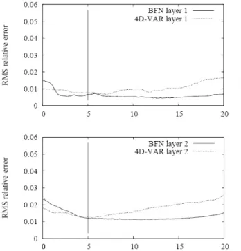
Fig. 2 – Evolution in time of the RMS relative difference between the reference trajectory and the identified trajectories for the BFN (solid line) and 4D-VAR (dotted line) algorithms, versus time, for each layer: from surface (1) to bottom (3).
Figure 2 shows, for each of the three layers, the RMS relative difference between the BFN trajectory (computed using the last BFN state at time t=0 as initial condition) and the reference trajectory as a solid line, and between the 4D-VAR trajectory (computed using the last initial state produced by the minimization process) and the reference trajectory as a dotted line, versus time. The first 5 days correspond to the assimilation period, and the next 15 days correspond to the forecast period.
The first point is that the BFN and 4D-VAR reconstruction errors have similar global behaviours: first decreasing at the beginning, during the assimilation period, and then increasing over the forecast period (see e.g. (Pires et al., 1996) for a detailed study of the 4D-VAR estimation error). Even if the reconstruction error on the initial condition is much higher with the BFN algorithm than with 4D-VAR, the BFN error decreases much more steeply and for a longer time than the 4D-VAR one, and increases less quickly at the end of the forecast period. The quality of the initial condition reconstruction is better using the 4D-VAR algorithm, but the BFN algorithm provides a comparable final estimation, and even a better forecast.
Another interesting point is that, even if only surface observations are assimilated, the identification of the intermediate and bottom layers is quite good. The 4D-VAR algorithm was already known to propagate surface information to all layers (Luong et al., 1998), but it is also the case for the BFN algorithm, even if this algorithm is less efficient on the bottom layer.
5. Conclusions
We have proved on several idealized situations that, provided that the feedback term is large enough as well as the assimilation period, we have convergence of the algorithm to the real initial state.
Numerical results have been performed on Burgers, shallow-water and layered quasi-geostrophic models. Numerical tests are currently investigated on a full primitive ocean model (NEMO). Twice less iterations than the 4D-VAR are necessary to obtain the same level of convergence. This algorithm is hence very promising in order to obtain a correct trajectory, with a smaller number of iterations than in a variational method, with a very easy implementation.
References
Auroux, D., 2009: The back and forth nudging algorithm applied to a shallow water model, comparison and hybridization with the 4D-VAR. Int. J. Numer. Methods
Fluids, DOI:10.1002/fld.1980.
Auroux, D. and Blum, J., 2008: A nudging-based data assimilation method for oceanographic problems: the Back and Forth Nudging (BFN) algorithm. Nonlin. Proc.
Geophys., 15, 305–319.
Bao, J.-W. and Errico, R. M., 1997: An adjoint examination of a nudging method for data assimilation. Mon. Weather Rev., 125, 1355–1373.
Blayo, E., Verron, J., and Molines, J.-M., 1994: Assimilation of TOPEX/POSEIDON altimeter data into a circulation model of the North Atlantic. J. Geophys. Res.,
99(C12), 24691–24705.
Durbiano S., 2001: Vecteurs caractéristiques de modèles océaniques pour la réduction d’ordre en assimilation de données. Ph.D. Thesis, Univ. Grenoble, France. Le Dimet, F.-X. and Talagrand, O., 1986: Variational algorithms for analysis and assimilation of meteorological observations: theoretical aspects. Tellus, 38A, 97–110. Luenberger, D., 1966: Observers for multivariable systems. IEEE Trans. Autom.
Contr., 11, 190–197.
Luong, B., Blum, J., and Verron, J., 1998: A variational method for the resolution of a data assimilation problem in oceanography. Inverse Problems, 14, 979–997.
Pires, C., Vautard, R., and Talagrand, O., 1996: On extending the limits of variational assimilation in nonlinear chaotic systems. Tellus, 48A, 96–121.
Talagrand, O., 1981: A study of the dynamics of four-dimensional data assimilation.
Tellus, 33A, 43–60; On the mathematics of data assimilation. Tellus, 33A, 321–339.
Trélat, E., 2005: Contrôle optimal: théorie et applications. Vuibert, Paris.
Vidard, P.-A., Le Dimet, F.-X., and Piacentini, A., 2003: Determination of optimal nudging coefficients. Tellus, 55A, 1–15.