Sex Ratio Imbalances Among Children At Micro-Level: China And India Compared.

HAL Id: halshs-00296636

https://halshs.archives-ouvertes.fr/halshs-00296636

HAL is a multi-disciplinary open access archive for the deposit and dissemination of sci-entific research documents, whether they are pub-lished or not. The documents may come from teaching and research institutions in France or abroad, or from public or private research centers.

L’archive ouverte pluridisciplinaire HAL, est destinée au dépôt et à la diffusion de documents scientifiques de niveau recherche, publiés ou non, émanant des établissements d’enseignement et de recherche français ou étrangers, des laboratoires publics ou privés.

Sex Ratio Imbalances Among Children At Micro-Level:

China And India Compared.

Christophe Guilmoto, Sébastien Oliveau

To cite this version:

Christophe Guilmoto, Sébastien Oliveau. Sex Ratio Imbalances Among Children At Micro-Level: China And India Compared.. Population Association of America 2007 Annual Meeting, Mar 2007, New York, United States. �halshs-00296636�

Sex Ratio Imbalances Among Children At Micro-Level: China And India Compared.

Christophe Z Guilmoto and S. Oliveau Guilmoto@ird.fr; sebastien.oliveau@univ-provence.fr

Sex ratio in Asia

Sex ratio imbalances found in Asia are primarily due to the increasing proportions of sons among children in China and India.1 This gradual demographic masculinization over the last two decades results from the rapid progression in the number of sex-selective abortions aimed at ensuring the birth of male children. While other factors such as female infanticide or excess child mortality have played a sizeable role in the past in distorting sex ratios among the child population, the rise of pre-birth sex selection has entirely changed the situation. Sex selection through abortion –following detection of sex of the foetus– represents a technological breakthrough that has enabled millions of Asian couples to implement a new and more effective strategy of sex planning aimed at getting rid of unwanted female births.

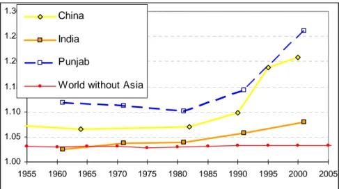
Figure 1 brings together child sex ratio estimates for China, India and the rest of the world (world without Asia). Sex ratio values (number of boys per hundred girls) around 107 have long been greater than normal in China, but the real increase dates from the 1980s. This change occurred at about the same period in India, although the magnitude of the rise in child ratio is much lower than in China. One reason for the slower increase recorded in India lies in the very uneven distribution of gender discrimination within the country. But as data for Punjab State in India indicates, regional values in India may be significantly higher than the Chinese average. In both Asian countries, the child sex ratio is probably still on the increase although lack of detailed annual series rules out any firm conclusion on most recent trends. During the last 40 years, the overall figure for the rest of the world has remained fairly stable at around 103, displaying almost no visible trend in sex ratio levels.

1.00 1.05 1.10 1.15 1.20 1.25 1.30 1955 1960 1965 1970 1975 1980 1985 1990 1995 2000 2005 China India Punjab

World without Asia

Figure 1: Child sex ratio in China and India, 1950-2000

This paper offers a comparative study of sex ratio distribution in China and India.2 We concentrate here on the measurement of sex ratio among the child population. Sex ratio imbalances among other, older age groups are more complex to interpret as they tend to be influenced by a host of other factors such as past trends in child sex ratio, sex-selective under-registration of young adults, adult mortality and sex-selective mobility behaviour (Bhat 2002).

Mapping child sex ratio

One puzzling aspect of sex ratio imbalances among children relates to its social and geographical distribution in both countries. Whenever data are available for specific household sub-populations, it appears that sex ratio imbalances are more acute visible among affluent, urban groups while being often negligible among underprivileged groups. To some extent, there appears also to be broad similarities between fertility change and gender discrimination. However, this relationship is far from straightforward as examples abound of groups combining both low (or high) fertility and gender discrimination levels (see also Bhat and Zavier 2003). But lack of age and sex data for household populations –that would allow us to estimate child sex ratio for populations classified by socio-economic status–often limits our capacity to assess the correspondence between class membership and discriminatory behaviour towards female births.

Geographical variations are on the contrary easier to highlight thanks to the availability of age and sex pyramids for various administrative levels such provinces/states, urban agglomerations, and lower-level regional units. Census data from China and India indicate for example that gender discrimination levels may be both extremely pronounced in several regions of East China and North-west India whereas the rest of these countries often exhibit normal sex ratio levels below 105. Punjab (Figure 1) where child sex ratio is presently greater than 125 illustrate the variations that may be found within a single country (see also Arokiasamy, 2004).

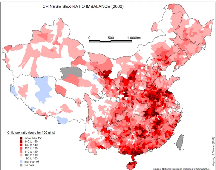
We start with detailed maps of both China and India based on results from the last census (see below for description of the data). The Chinese map (Figure 2) shows the great West-East division of the country in terms of child sex ratio. While its values tend to be usually normal in the western half of the country, the eastern half is characterized by high sex ratio levels. In East China, spatial patterns tend also to be more intricate. There are obviously several “hot spots” of masculinity in a few areas where values can at times cross the 150 mark. These areas are usually located away from the coast (except in South Guangdong and Hainan) as can be seen in Jiangxi or in Henan. The resulting picture remains fairly fragmented since hot spots may often be contiguous to areas where child sex ratio is at a normal level. We see several such instances of heterogeneity within Hubei, Anhui or Guangxi provinces.

2

For other comparisons between China and India, see Das Gupta et al. (2003), Guilmoto (2005) and Guilmoto and Attané (2005).

Figure 2: Child sex ratio in China, counties, 2000.

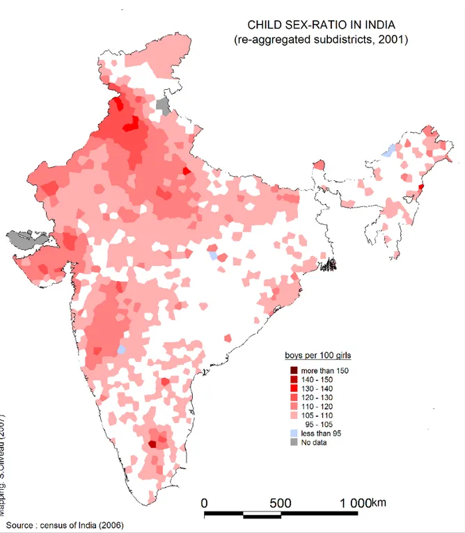
India’s map (Figure 3) tends to be much easier to decipher than China’s in spite of being based on a much larger number of units (see below for details). The vast majority of excess sex ratio values are shown to be clustering towards the Northwest. The highest values are recorded in the states of Punjab and Haryana, while other “core areas” may be found in Gujarat or Maharashtra. Interestingly enough, there appears to be a corridor of low child sex ratio separating North-western India from the contiguous state of Maharashtra where values are also high. This land strip closely corresponds to tribal settlements found at the borders of four States (viz. Rajasthan, Gujarat, Maharashtra and Madhya Pradesh) along the Narmada River basin. One may also distinguish in the map a few isolated hot spots such as in Tamil Nadu (Salem area) or in Orissa.

Figure 3: Child sex ratio in India, subdistricts, 2001.

The difference in spatial patterning observed in China and India may seem rather perplexing. China is to a large extent socially and culturally more homogeneous than India. Religious and linguistic differences tend for instance to be significantly more acute across regions in India than in East China which is overwhelmingly Han–populated (with standard Mandarin widely understood). Consequently, we would expect demographic behaviour to be more homogenously distributed in China. Mapping sex ratio at a fine level shows on the contrary a large amount of local disparities within Chinese provinces. We may therefore wonder whether the fragmented picture of China’s sex ratio differentials is actually linked to local factors. Among possible such factors, local variations in family policy enforcement may explain why some localities would have very different demographic outcomes than their neighbours.

Another hypothesis relates to differentials in registration level caused by under-reporting of girls either by local population or by government officials.

There may however be another explanations for local irregularities. This is best illustrated by India’s map: in it, we see that Andhra Pradesh’s distribution of sex ratio values is rather erratic in stern contrast to the rather regular geographical repartition observed elsewhere. Similar observations could be made for other states such West Bengal or Arunachal Pradesh. As we will show below, this irregular distribution is not caused by demographic behaviour, but rather by the insufficient demographic size of administrative units that have been mapped. This means that plotting values for small units as was done in the two previous maps may result in artificial statistical distortion when estimating local child sex ratio. Such local heterogeneity visible in some areas would then disappear when maps are based on larger units that tend to blur out local irregularity. Another consequence is that comparing China’s sex ratio map with India’s may not be advisable as long as administrative units for both countries are too dissimilar in both population size and area.

Measuring sex ratio

In this section, we will go back to our original datasets and describe them in greater detail. The last census was conducted respectively in 2000 in China and 2001 in India. No other data set provides an exhaustive sex and age count for both national populations. While China follows standard age classification (below 1 year, 1-4 years, 5-9 years etc.), India’s data are not always available in the customary quinquennial age format. For some units, figures given by the Census relate to the populations aged “less than 7 years” or “7 years and more” as the latter age group is used to compute literacy rates. But we may add that because of the relatively high level of age heaping in India –also associated to sex of the children such as for exact age 5-, the 0-6 year age group tends to offer a more robust measurement of sex ratio than the usual 0-4 group. Another advantage relates to the larger size of the 0-6 age segment used to compute sex ratio (more on sex ratio variability below). China’s age data are however on the whole of much better quality than their Indian counterparts. The difference in age group between countries may however have little impact in our comparison since adding ages 5 and 6 is unlikely to alter the overall sex ratio among children.

Child sex ratio itself happens to be a rather synthetic measure of gender discrimination as it incorporates the impact of its three main components: skewed sex ratio at birth, infanticide and sex differentials in infant and child mortality. At the same time, it is not known to be significantly affected by differentials in migration that may deeply alter sex ratio among older age groups. However, computation of sex ratio necessitates relatively large population sizes especially because it is a ratio (with both fluctuating denominator and numerator) and not a rate. A simple sensitivity analysis using the binomial distribution shows for instance that sex ratio fluctuates widely for smaller populations: for a population of 10,000 (and assuming a theoretical sex ratio of 105), the 95% confidence interval for the sex ratio is [99.3-111]. This militates against extending the geographical analysis to very small administrative units as random variations related to sample size may result in artificially high levels of local variability of sex ratio estimates.

Data from these censuses are available at various administrative levels in both countries. In China, the larger units are the 33 province-level units (provinces, municipalities and other regions), further divided into 333 prefectures while the finer units correspond to counties (Xiàn). There were 2391 counties in China at the time of the 2000 census out of which 2368

spatial units could be retained in this study.3 In India, sex ratio data have long been examined on the basis of the 35 States and Union Territories or of the 593 districts existing during the 2001 census. This smaller number of districts in India, compared to China’s counties, means that district units tend to be much larger in terms of population and are not directly comparable to China’s counties.

Recently, data for so-called subdistrict units have been made available (CensusInfo 2005) for India. These units are identified in most States as “tahsils” although there are many other regional appellations such as “taluks” (in several south Indian states), “mandals” (Andhra Pradesh), “CD-blocks” in Bihar or West Bengal, “circles” in North-eastern India, etc. The main advantage of this subdistrict series that include the population below 7 is that they correspond to 5564 units, almost ten times more than districts. This grid has been used for the map of child sex ratio shown at the beginning of the paper. This administrative level combines however different regional administrative grids that tend to vary widely in area across Indian states. For instance, the 1125 mandals found in Andhra Pradesh are extremely small units. But the existence of such data (which have been further georeferenced by the authors using Census of India sources) will provide us the best dataset to confront local sex ratio variability in both China and India.

Geographical and administrative differences between China and India

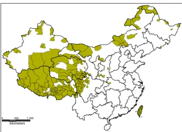
Geographically, China and India present much dissimilarity. On the whole, the spatial distribution of the population tends to be highly skewed in China towards the Eastern part of the country where human density is extremely high. Large parts of China’s western provinces (such as Xinjiang or Tibet) display on the contrary very low population density levels. They mostly correspond to barren, arid tracts where cultivable land represents less than 5% of the overall land surface. As a result, counties in Western China are often gigantic though possessing tiny populations. In 156 counties, the area exceeds 10,000 sq. km. Almost 400 counties have a child population that is below 10,000. Figures 4 and 5 indicate that these counties are mostly located to the West of the country.

0 500 1 000

kilometers

Figure 4: Chinese counties with area above 5000 sq. km

3

0 500 1 000

kilometers

Figure 5: Chinese counties with child population below 10,000.

Data shown on Table 1 show that Chinese counties are on average much larger in area than their Indian counterparts, but also that they are characterized by a sizeable standard deviation resulting from differences between the western and eastern parts of China. A further source of complication stems from the fact that these counties with large land area but limited population are also characterized by the lowest sex ratio observed in the country. Not only are minority groups often more numerous than ethnic Hans in these parts of the country, but fertility levels are on the whole higher than in the rest of the country. These areas are also predominantly rural and underdeveloped. These various features explain why child sex ratio in these low-density regions is at its lowest, but the combination of spatial and demographic features may also be seen as a potential source of trouble for spatial comparison.

Country

Name of lower

-level units Number Number of

units used for this study Area (sq. km) Number of units

with area Child population Number of

units with less tha n 1000 0 children >10000 sq. km >5000 sq. km <500 sq. km

China Counties (Xiàn) 2,391 2,368 Av: 3,807

Sd: 11,473 156 308 400 Av: 29,093 Sd: 25,914 398 India Subdistricts (Tehsils, taluks, mandals, etc.) 5,564 5,454 Av: 579 Sd: 1,314 2 14 3290 Av : 28,806 Sd: 36,741 1,655 China Re-aggregated counties 1400 Av 3,096 Sd: 2,902 11 102 5 Av : 45,790 Sd: 42,893 127 India Re-aggregated subdistricts 1512 Av : 2,142 Sd: 2,391 3 17 8 Av : 105,134 Sd: 117,224 64

Notes: Av: average value; Sd: standard deviation.

Table 1: Characteristics of lower-level administrative units, China (2000) and India (2001)

While not absent, variations in density levels across regions in India are far less pronounced than In China. Moreover, they do not correspond in any way to variations in child sex ratio levels and density heterogeneity is therefore unlikely to impact on variations in sex ratio as may be the case for China. However, the problem of small units is more acute for India where subdistricts often have limited population. As maps on Figures 6 and 7 illustrate, small and underpopulated subdistrict units tend to coincide in India, being clustered in Andhra Pradesh, Bihar or in North-East States such as Arunachal Pradesh or Nagaland. No less than 1655 subdistricts in India have a child population below 10,000 and they account for 30% of the overall number of subdistrict units. An even larger proportion of subdistricts have an area smaller than 500 sq. km.

Figure 6: Indian subdistricts with area below 500 sq. km.

Why do these differences in administrative structures matter? The first reason relates to the above-mentioned variability of sex ratio. If computed on small populations (such as localities with less than 10,000 children), sex ratio may take values affected by sizeable random errors. Another less obvious reason corresponds to the geographical processes that are captured in spatial analysis. In the geostatistical investigations that will follow, we will examine how far sex ratio observed in different units are affected by sex ratio values observed in other neighbouring administrative units. We will thus examine how far distance impacts on sex ratio variations. But distance across units is closely related to their average size: large regions are spatially more distant from each other than smaller ones lying closing to each other. If we want to examine the impact distance has on sex ratio variations within countries, we should therefore avoid using heterogeneous administrative grids combining very large and small units. This is especially true when the average area of administrative units tends to be correlated with the feature studied (here, child sex ratio). Moreover, to compare geographical distribution in both countries suggest using comparable units and India’s are obviously too small in several regions.

The administrative grids in China and India are therefore too dissimilar to allow for direct comparison and some units appear also to be either too large or too small:

• Some units (mostly in China) that may be too large as well as underpopulated • Some units (mostly in India) that may be too small as well as underpopulated

These problems call for different solutions. About China’s large underpopulated countries, the only way was to remove from our study the provinces where they are found. We decided therefore to restrict our study to Central and Eastern China and remove the provinces of Xinjiang, Xizang (Tibet), Qinghai, Gansu and Nei Menggu (Inner Mongolia).4 These provinces account for no more than 6% of China’s overall population. Provinces retained in our analysis correspond roughly to the eighteen historical Chinese provinces (Qing Dynasty), to which have been added the northeastern provinces.

As for administrative units where population was deemed too small, we used spatial analysis tools to re-aggregate units using spatial proximity. The basic idea consists in merging counties that were close to each other and create a new spatial dataset made of slightly larger units. To do this, we have used Voronoi polygons to club together units according to their proximity. This method not only tends to reduce the number of small, underpopulated units where sex ratio computation may be fraught with estimation uncertainty, but it also produces new datasets for China and India that tend to be more similar in terms of average area.

After a few trials, it was decided to merge units that were less than 30 kilometres apart. This distance range has effectively reduced the number of underpopulated units from our original sample. Results shown on Table 1 above indicate that our new datasets for China and India are now of better quality and much more homogenous across countries. Because of spatial re-aggregation procedure followed, the number of small units has drastically declined in both countries. This reflects on the number of units with child population below 10,000: they have almost disappeared in India while their proportion has greatly declined in China. We may however note that even after re-aggregation, there subsist a few units that are oversized or underpopulated in China and this is mostly caused by the presence of units located along the western border.

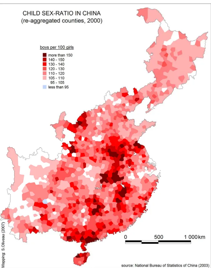
The number of units is now similar for both countries (1400 for Eastern China and 1512 for India) and the average area of these re-aggregated units is comparable (3,096 sq. km for China as against 2,142 for India). This procedure allows us now to compare more confidently the spatial distribution in both Asian countries using a new set of map based on re-aggregated units (Figures 8 and 9).

The new map of East and central China’s sex ratio (Figure 8) is now easier to interpret as many local differentials have vanished. However, the patchy distribution of sex ratio values remains a major trait of China’s map as no clear-cut geographical patterns has emerged.

Figure 9: Child sex ratio in India, re-aggregated subdistricts, 2001.

The new map drawn for India (Figure 9) has suppressed most local irregularities. This can be seen from Andhra Pradesh where sex ratio values are now uniformly below average except for a small pocket towards the South that was previously invisible. Similarly, the picture from States such as Bihar and West Bengal are now easier to interpret. The tribal corridor hinted at earlier that separates North-western India from Maharashtra remains clearly distinguishable.

Local autocorrelation

To go beyond the mere visual inspection of maps, we will resort to geostatistical tools to identify more systematically masculinity hot spots. Using Anselin’s definition of local indicators of spatial association, we now submit our maps to the examination of local patterns. Each unit is now tested for local spatial autocorrelation (Anselin, 1995, 2003).5

We start with a comparison between observed values and values obtained in neighbouring units. The procedure is also known as Moran’s scatterplots. To do that, we’ll use two different definitions of “neighbourhood”. The first definition limits the notion of neighbours to that of immediately spatially adjacent units. The second, more comprehensive treatment of neighbourhood rests on third-order contiguity: units need to have less than 3 units between themselves to qualify as “neighbours”. The resulting plots shown on Figures 10 and 11 show local values (X-axis) to be strongly correlated to that of their neighbours (Y-axis). The correlation is as expected stronger for a restrictive definition of neighbourhood based only on adjacent units.

Figure 10: Moran scatterplots for China and India, first-order contiguity.

5

See also Bailey & Gatrell (1995), Haining (2003) and Goodchild & Janelle (2004) on spatial autocorrelation measurement and interpretation.

Figure 11: Moran scatterplots for China and India, third-order contiguity.

Comparing now China to India, we see almost similar patterns of correlation at least using first-order contiguity. Moran’s I (here computed following Anselin’s formula), which corresponds to the fit of the scatterplots, is very high for both countries and at almost similar levels (.693 for India vs. .646 for China). In other words, in both China and India, there is a strong level of spatial dependency as far as gender discrimination is concerned: the correlation between adjacent units means that strictly local variations in sex ratio levels are uncommon. This of course calls to mind the possible role of diffusion processes to explain how local gender attitudes tend to be so homogeneous on this scale.

The difference between China and India appears more significant when we use a higher-order contiguity definition for neighbourhood. This implies that spatial autocorrelation tends to decrease faster in China and that distance has a stronger impact on heterogeneity between administrative units. However, Moran’s values remain strong and significant even for distant neighbours.

Using scatterplots, we may now define hot spots as areas where child sex ratio values are the highest with neighbouring values also high (“high-high”, in red on figure 12 & 13). In the same vein, “cold spots” can also be identified where sex ratio is below average in both individual units and their neighbours (“low-low”, in blue). A more generous definition of neighbourhood –based on third-order contiguity– logically results in a larger number of hot spots. In India we distinguish the two core regions previously mentioned: North West India as well as inner Maharashtra. Other areas with high sex ratio tend to be too small to show up on the map of hot spots. A very large region extending from Kerala to the Southwest towards Northeast India is on the contrary characterized by homogenous, lower than average sex ratios.

Figure 12: Child sex ratio hot spots in China, third-order contiguity.

Figure 13: Child sex ratio hot spots in India, third-order contiguity.

In China, the largest sex ratios belong to a large strip stretching from Hainan in the South to Henan in Yellow River Valley. This zone remains however slightly fragmented with lower than expected sex ratio (or spatial outliers) found in many interstices. Apart from parts lying along the Western border of our China map, there are several regions with homogeneous low

sex ratio values such as the North-eastern states. Another visible such region is found in one of China’s most modernized area, i.e. the Yangtze River delta in Shanghai and Zhejiang provinces.

Discussion

This paper has attempted to examine the spatial patterns of gender discrimination in China and India using geostatiscal tools that are becoming more common in demography (Voss et al. 2006). Spatial distributions of child sex ratio in both countries are rather dissimilar. India’s patterns are oriented towards the Northwest whereas East China is characterized by a larger number of distinct hot spots. These differences may be related to the process through which gender discrimination has emerged in China and India. At the same time, it is also possible that such spatial variations between China and India could be partly artificial, resulting from the specific characteristics of each national administrative grid.

To examine the latter hypothesis, this paper has sought to harmonize the administrative grid in both countries. To do that, we have used for the first time India’s subdistrict map that offers a much finer level of detail than district-based maps that are typically used. We have then conducted a re-aggregation procedure for both countries, after removing China’s western provinces where population is too sparse. Results presented above are therefore less likely to be influenced by specific national administrative grids. Moreover, since the units used are of roughly comparable characteristics, the comparison of spatial autocorrelation across countries is now less risky.

What emerges is that local spatial autocorrelation at short distances is almost as strong in China as in India. In both countries, local sex ratio values tend to be closely correlated to values observed in neighbouring localities. This geographical clustering is a typical feature of sex ratio degradation in Asia and directly refers to the diffusion process of discriminatory behaviour. While it may be in theory conceivable that such spatial patterning proceeds from the spatial distribution of other characteristics, previous analysis has failed to identify any likely determinant that would explain away this peculiar spatial distribution.

In India’s case, for instance, spatial autocorrelation has regularly been shown to be an irreducible component of regional variations in sex ratio levels (Kishor 1993; Murthi et al. 1995: Malhotra et al. 1995). To take one example related to the religious factor, high sex ratio in Punjab is often related to the spatial distribution of the Sikh population among which female discrimination is intense. But by the same token, maps demonstrate that child sex ratio in neighbouring Haryana state, which is strongly Hindu-dominated, is equally as high. Likewise, child sex ratio among Muslim communities, which as a whole records low sex ratio values in India, tends to be significantly higher in the Northeast than elsewhere. Another important feature of child sex ratio in India is that it turns out to be the most spatially autocorrelated variable (Oliveau and Guilmoto, 2005), which suggests that spatial patterns observed for child sex ratio are unlikely to be the sheer corollary of spatial patterns of some other factor.

Correlates of high sex ratio in China are often far less established than for India. Within Han-dominated areas, incriminated factors such as low fertility, family patterns, urbanization or socio-economic status seem to play but a minor role if any (Lavely and Cai, 2004). This leaves spatial clustering partly unexplained by social or economic factors and regression residuals remain spatially autocorrelated. Differential registration levels at the local level may be a

hidden factor, but there is somewhat conflicting evidence on this aspect.6 Moreover, the rather strong spatial regularity of sex ratio differentials within East China in 1990 and 2000 suggests that local factors are not spurious. Moreover, strong spatial autocorrelation at the local level indicates that these other factors –such as variations in reporting levels– would exhibit spatial autocorrelation, a feature that may sound rather unlikely. Variations in the quality of registration tend indeed to be rather random and not permanent over time. Other unobserved factors may be ultimately to sub-ethnic value systems with Han China on which we have little testable information. There seems to be however no direct connection between Chinese dialect geography and sex ratio distribution.

These observations reinforce the hypothesis that spatial patterns closely reflect the mechanisms behind the propagation of discriminatory behaviour in both India and China during the last three decades. Several factors often thought to fuel discrimination such as availability of new technologies (scanning and abortion facilities) would tend to level off spatial differentials or to determine on the contrary a strong urban bias as technology diffusion proceeds in a top-down manner along the urban hierarchy. But no such urban bias can be detected from our maps. Fertility decline is also poorly correlated to local variations in sex ratio differentials and the correlation is at times presumed to be curvilinear (Lavely and Cai, 2004; Legge and Zhao, 2004), a feature most likely to disturb modelling attempts. Several instances of early declining regions such as Kerala in India or Shanghai in China do not indeed exhibit any substantial levels of discrimination towards girls.

The role of cultural macro-regions from where discriminatory practices seem to originate is a much more plausible factor behind the observed spatial distribution in India. Discriminatory attitudes and technology has diffused from core regions towards culturally homogeneous, adjacent regions over the years. New hot spots that have recently emerged such as in coastal Orissa are therefore likely to expand mechanically towards neighbouring regions. There is an unmistakable aspect of laissez-faire in the way demographic outcomes evolve in India, more often guided by changing level of demand than by supply factors or government intervention. But in China, these regions appear to be smaller in size and their impact on neighbouring areas appears more limited than in India. The somewhat fragmented pattern obtained in the latter country probably relates to the strong capacities of local and regional authorities to influence demographic outcomes. Local enforcement of regulations of family planning or sex-selective abortion, not to mention local abilities to distort census data, do not however extend over distant zones and proceeds from entirely different mechanisms than unrestrained diffusion processes across social groups and localities as observed in India. Wide market mechanisms in India vs. local official regulations in China may therefore explain to a large extent the differences in spatial patterns in child sex ratio observed between both countries.

Bibliography

Anselin, L., (1995), « Local indicators of spatial association - LISA », Geographical Analysis, Vol. 27, n°2, pp. 93-115.

Anselin, L., 2003, GeoDa 0.9 User’s Guide. Spatial Analysis Laboratory (SAL), Univeristy of Illinois at Urbana-Champaign.

Arokiasamy, P. 2004, “Regional patterns of sex bias and excess female child mortality in India” Population-E, 59(6), 833-864.

6

Attané, I., Véron, J., eds., 2005, Gender issues at the early stage of life in South and East Asia, IFP-CEPED, Pondicherry.

Bailey, T. C., and Gatrell, A. C., 1995, Interactive Spatial Data Analysis, Longman, Harlow.

Bhat, PN Mari and AJF, Zavier, 2003, ‘Fertility Decline and Gender Bias in Northern India’, Demography, Vol. 40, No. 4, 637-657.

Bhat, PN Mari, 2002, “On the Trail of ‘Missing’ Indian Females”, Economic and Political Weekly, December, 5105-5118 and 5244-5263.

CensusInfo, 2005. CD-ROM, version 2, Office of the Registrar General, India, New Delhi.

Chu, Junhong, 2001. “Prenatal sex determination and sex-selective abortion in rural central China”. Population and Development Review, 27, 2, 259-282

Croll, E. 2000, Endangered Daughters: Discrimination and Development in Asia, London and New York: Routledge.

Das Gupta, M., et al., 2003,. "Why is son preference so persistent in East and South Asia?: A cross-country study of China, India and the Republic of Korea," Journal of Development Studies. 40, 2. Goodchild, M.F., Janelle, D.G., (2004), Spatially Integrated Social Science, coll. Spatial Information

Systems, Oxford University Press, New York, 456 p.

Guilmoto, C.Z. and I. Attané, 2005. “The geography of deteriorating child sex ratio in China and India”, communication to the International Population Conference, Tours, July.

Guilmoto, C.Z., 2005. "A spatial and statistical examination of child sex ratio in China and India”, in Attané, I. and J. Véron, eds., Gender discrimination among Young Children in Asia, French Institute of Pondicherry and CEPED, Pondicherry, 133-167.

Haining, Robert, 2003, Spatial Data Analysis: Theory and Practice, Cambridge University Press, Cambridge.

Kishor, S., 1993, “"May God Give Sons to All": Gender and Child Mortality in India”, American Sociological Review, 58, 2, 247-265.

Lavely, William and Cai Yong, 2004. “Spatial Variation of Juvenile Sex Ratios In the 2000 Census of China”, presentation at the annual meeting of the Population of Association of America, Boston, April 1-3

Legge, Jerome S. Jr. and Zhirong Zhao, 2004. “Morality Policy and Unintended Consequences: China’s “One-Child” Policy”, Chinese Public Administration Review, 2 · 3/4 · September/December, 30-54.

Li, Shuzhuo, et al., 2004. “Gender differences in child survival in contemporary rural China: a county study”, Journal of Biological Science, 36(1), 83-109.

Malhotra, A. et al., 1995, “Fertility, Dimensions of Patriarchy, and Development in India”, Population and Development Review, 21, 2, 281-305.

Merli, 1998, “Underreporting of Births and Infant deaths in Rural China: Evidence from Field Research in One County of Northern China”, China Quarterly, 155, 637-655.

Merli, M. G., and Raftery, A. E., 2000, “Are Births Underreported in rural China? Manipulation of Statistical Records in response to China’s Population Policies” Demography, 37, 1, 109-126. Murthi, M., et al., 1995, “Mortality, Fertility, and Gender Bias in India: A District-Level Analysis”,

Population and Development Review, 21, 4, 745-782.

Oliveau S. and Guilmoto, C.Z., 2005. « Spatial autocorrelation and demography. Exploring India’s demographic patterns », communication to the International Population Conference, Tours, July.

Voss, Paul R., Katherine J. Curtis White, and Roger B. Hammer, 2006, “Explorations in Spatial Demography.” in William Kandel and David L. Brown (eds.), The Population of Rural America: Demographic Research for a New Century. Dordrecht, The Netherlands: Springer, 407-430. Wu, Zhuochun et al., 2006 “Determinants of High Sex Ratio among Newborns: A Cohort Study from