HAL Id: hal-00642699
https://hal.archives-ouvertes.fr/hal-00642699
Submitted on 18 Nov 2011
HAL is a multi-disciplinary open access
archive for the deposit and dissemination of sci-entific research documents, whether they are pub-lished or not. The documents may come from teaching and research institutions in France or abroad, or from public or private research centers.
L’archive ouverte pluridisciplinaire HAL, est destinée au dépôt et à la diffusion de documents scientifiques de niveau recherche, publiés ou non, émanant des établissements d’enseignement et de recherche français ou étrangers, des laboratoires publics ou privés.
Financial and Economic Determinants of Firm Default
Giulio Bottazzi, Marco Grazzi, Angelo Secchi, Federico Tamagni
To cite this version:
Giulio Bottazzi, Marco Grazzi, Angelo Secchi, Federico Tamagni. Financial and Economic Determi-nants of Firm Default. Journal of Evolutionary Economics, Springer Verlag (Germany), 2011, pp.373. �hal-00642699�
Financial and Economic Determinants of Firm Default
∗
Giulio Bottazzi
†◦, Marco Grazzi
◦, Angelo Secchi
§, and Federico Tamagni
◦◦
LEM, Scuola Superiore Sant’Anna, Pisa, Italy
§Universit`a di Pisa, Pisa, Italy
December 9, 2010
Abstract
This paper investigates the relevance of financial and economic variables as deter-minants of firm default. Our analysis cover a large sample of medium-sized limited liability firms. Since default might lead, through bankruptcy or radical restructuring, to firm’s exit, our work also relates with previous contributions on industrial demography. Using non parametric tests we assess to what extent defaulting firms differ from the non-defaulting group. Bootstrap probit regressions confirm that economic variables, in addition to standard financial indicators, play both a long and short term effect. Our findings are robust with respect to the inclusion of Distance to Default and risk ratings among the regressors.
JEL codes: C14, C25, D20, G30, L11.
Keywords: firm default, selection and growth dynamics, stochastic equality, bootstrap probit regressions, Distance to Default, credit rating.
∗We would like to thank the attendants of the “Revolving Doors” conference for useful suggestions on a
preliminary version of the paper. The final version benefits from the insightful hints of Elena Cefis and two anonymous referees. The research leading to these results has received funding from the European Commu-nity’s Seventh Framework Programme (FP7/2007-2013) under Socio-economic Sciences and Humanities, grant agreement n 217466
1
Introduction
Business failures have been the subject of extensive analysis in applied economics and econo-metrics. One obvious reason is that the “death” of a firm represents the ultimate market response to the inability of an economic activity to survive the competitive pressure. In this sense the study of business failures essentially rests on the more general issue of identifying which characteristics make a given firm, or group of firms, more or less competitive. At the same time, the failure of a business activity represents an unnecessary, or at least avoidable, waste of tangible and intangible assets, something that entrepreneurs, managers, firms’ credi-tors, employees and the society as a whole would surely had preferred to avoid. Clearly, our ability to design policies in order to minimize the occurrence, or the effects, of this unwanted event depends on our understanding of the original and contingent determinants of firm death. Traditionally, industrial economic literature studied firm’s death, using the “exit” event as reported in business registers. From an economic point of view, however, these events are often spurious. They might be in fact associated with a simple relabeling of the economic subject, following a change of ownership or a modification of incorporation status. These changes do not imply any economic effect on business operations, nor signal any actual difficulty on the part of the firm. Moreover, even when the exit is real, it can take various forms, like voluntary liquidation, acquisition or bankruptcy. These forms of exit represent very different economic outcome and are likely to be caused by different factors. Despite these differences, most of the existing literature has treated exit as a homogeneous event (see, for instance, Dunne et al. (1988), Mata and Portugal (1994) and Disney et al. (2003)). Recent contributions (Honjo, 2000; Cefis and Marsili, 2007; Esteve-P`erez et al., forthcoming) try to distinguish between the different routes to exit, but are still limited by the difficult interpretation of the related legal events (restructuring, acquisition, merger, etc.) and by their exact timing. Indeed, when a firm is about to exit the market, information get more scarce, and it becomes difficult to determine with precision when operations actually ceased.1 Of course being unable to exactly
determine the time of the exit severely constraints the possibility to realize large scale study (a case to the point are, for instance, the works by Schary, 1991; Agarwal and Gort, 1996; Audretsch et al., 1999).
In this paper we use a different strategy to study the issue. We exploit information on distress events occurring in a large panel of Italian firms and identify potential business failures with financial defaults. A default is considered to have occurred when the obligor is past due more than 90 days or when the bank considers that the obligor is unlikely to repay its debt in full (BIS, 2006).2 Like firm failures, default events are both a signal of business troubles
and a costly condition that should be in principle avoided. Even if default is not directly related with exit, it constitutes the main requisite for starting the bankruptcy procedures.3 If
a defaulting firm is not filed for bankruptcy4 it is then very likely that it goes through a process
1
Bankruptcy procedures might procrastinate for years before they conclude and the exiting firm is eventually deleted from the register. In Italy, for instance, it took on average more than 7 years, in 2004, for bankruptcy procedures to get to an end (ISTAT, 2006).
2
Such conditions might slightly vary, depending on the internal regulations of every single bank. Since we consider here only default event collected by a single bank, we confront ourselves with a homogeneous definition.
3
According to the Italian civil law there is a subjective and an objective requisite for accessing bankruptcy law. The former is the professional nature of the activity and the latter is insolvency. The subjects entitled to appeal for the application of bankruptcy law are the firm itself, the bank or other creditors.
4
The evidence suggests that not always subjects involved find it convenient to apply for bankruptcy law (Shrieves and Stevens, 1979; Gilson et al., 1990; Gilson, 1997; Hotckiss et al., 2008).
of profound restructuring, also resulting in a substantial change in the ownership of the firm (Cefis and Marsili, 2007; Hotckiss et al., 2008), or that it is interested by some forms of merger and acquisition (M&A). As a result the event of default is strictly related to the “involuntary” modes of exit identified in the literature of industrial demography (Schary, 1991). Moreover, since firm solvency condition is strictly monitored by lending banks, the default condition is precisely identified in time.
The firm default has been extensively studied in the literature devoted to banking and corporate finance, where it is used as one of the main indicator of financial distress. This literature has traditionally investigated the relation of default events with various financial variables (leverage, cost of debt, debt time structure, etc.) often with the aim of developing a synthetic rating measure capable to account for the risk involved in financing a particular business activity (see Beaver (1966) and Altman (1968); and Altman and Saunders (1998) and Crouhy et al. (2000) for a review). In these models firm distress is typically conceived to be primarily determined by poor financial conditions, especially in the short run before default occurs. Purely industrial factors tend to receive less attention and sometimes turn completely left out of the analysis. The best example is provided by the development of the “Distance to Default” (DD) model which prices the market value of a firm as a call option on the value of the firm, with strike price given by the face value of its liabilities (Black and Scholes, 1973; Merton, 1974). The idea is that the owner exercises her right to operate the firm if the (properly discounted) expected future revenues generated by its activities are higher enough to offset firm’s liability and the revenues obtained with the present liquidation of its assets. Under the assumption of efficient markets, the value of firm’s equity, the market values of its assets and the face value of its debt are enough to derive its probability to default over a given time horizon.
In the present work we start by focusing on those variables that are generally proposed in the literature of financial economics as explanatory of firms default. Yet, while the financial nature of default events clearly suggest to look primarily for short-term financial causes, it is well understood that the probability to stay in the market, as well as the financial stability of a firm, is deeply intertwined with the ability to perform well along the economic/industrial dimensions of its operation. Thus, it is likely that looking exclusively at financial indicators cannot offer but a partial account of the main determinants of default, at least as long as market frictions or other institutional factors are affecting the extent and the speed to which economic performances get perfectly reflected into financial structure and financial conditions.5
For this reason we will augment our initial purely financial models with a set of economic predictors, including productivity, profitability, size and growth variables, which are likely to be significantly related with firms’ success (and failure). Indeed, despite different schools of thought exist on the theory of the firm, there is strong agreement that the variables above represent the key levels of corporate performance along the selection process.6
A remarkable feature of the present analysis rests in its wide scope. While typical studies of firm default focus on large publicly traded companies, our study covers almost 20,000 limited liabilities firms active in manufacturing, very different in size and type of activity. This makes our study highly representative of the dynamics of Italian industry. Moreover, the
5
Starting from similar considerations Grunert et al. (2005) propose an “augmented” version of a standard financial model of default prediction which also includes two “soft” non-financial characteristics (managerial quality and market position) among the regressors.
6
The same message is consistent with broad sense neoclassical models of firm-industry dynamics (see, for instance, Jovanovic, 1982; Ericson and Pakes, 1995; Melitz, 2003), as well with models originating from the evolutionary tradition (see Winter, 1971; Nelson and Winter, 1982).
contemporaneous analysis of financial and economic variables, allows us to bridge the financial and industrial literature on, respectively, default and exit.7
We offer two specific contributions. First, we explore the heterogeneities possibly existing both within and across defaulting vis ´a vis non-defaulting firms along each dimension consid-ered. We estimate the empirical distribution of their financial and economic characteristics, and employ non-parametric tests for stochastic equality to measure variation of results near to default vs. further away from it. Second, and in accordance with the main purpose of the paper, we estimate a series of probit models of default probability, allowing us to identify which are the main determinants of default once the effects of economic and financial factors are allowed to simultaneously interplay. Bootstrap techniques are used to obtain robust es-timates of the relevant coefficients, and a set of model evaluation criteria is also introduced, enabling to discern if default prediction accuracy is improved when economic characteristics are added to financial factors.
The analysis of empirical distributions reveals that defaulting and non-defaulting firms display important differences along both economic and financial characteristics. Further, re-sults from bootstrap probit regressions reveal that the impact on the probability of default exerted by economic characteristics remains significant even near to default, when one would instead expect that economic factors have been already embodied into financial conditions. The findings do not change when we add, among the regressors, an approximate measure of Distance to Default and an official credit rating index. This supports the robustness of our conclusions with respect to the inclusion of further dimensions which we might not directly capture through the set of financial and economic variables available to us. All the results do not depend from sectoral specificity at the level of 2-Digit industries.
The rest of the work is organized as follows. Section 2 presents a detailed description of the dataset. A first descriptive comparison of defaulting v s non-defaulting firms is provided in Section 3, based on kernel estimates of the empirical distributions of economic and financial variables in the two groups of firms. Section 4 further explores the issue by means of more formal statistical tests of distributional equality. In Section 5 we tackle bootstrap probit estimates of default probability, focusing on whether the addition of economic variables can improve the explanatory and predictive power of the models, as compared to a benchmark specification where only financial indicators are used. Robustness of results with respect to the inclusion of Distance to Default and credit ratings is then tested in Section 6. Finally, Section 7 concludes suggesting some interpretations.
2
Data, variables and sample selection
The present analysis is based on a list of default events occuring within Italian manufacturing in either 2003 or 2004. These events are independently provided by an Italian bank (labeled “Bank” in what follows) only for those firms which were among its customers. The list is linked with information obtained from the Centrale dei Bilanci (CeBi) database, which contains financial statements and balance sheets of virtually all Italian limited liability firms. Italian Civil Law enforces the public availability of the annual accounting for this category of firms. CeBi collects and organizes this information, performing initial reliability checks.
7
A huge empirical literature has highlighted the positive effect exerted on survival by the technological characteristics of the firms, like R&D expenditures or patents (see Agarwal and Audretsch, 2001, for a review). Unfortunately we lack the necessary data to include these further dimensions in our analysis (see details in Section 2).
The database is quite rich and detailed and includes firms operating in all industrial sectors without any threshold imposed on their size. This represents a remarkable advantage over other firm level panels, which typically cover only firms reporting more than a certain number of employees, and makes it particularly suitable for the analysis of both large and small-medium sized firms.
Merging the list of defaults made available by the Bank with CeBi data provides the final dataset. This contains balance sheet information for manufacturing firms over the period 1998-2003 with the addition of a dummy variable taking on value 1 when a firm appears in our list, i.e. incurs default at the end of the period (in either 2003 or 2004), and 0 otherwise.8 Since
the list contains only customers of the Bank, some end-of-period defaulters can be present in the CeBi database, which are not in our list. It is therefore likely that our dataset understates the frequency rates of default actually occurring in the population. This is common problem in studies of distress prediction, potentially problematic for regression analysis, as incorrect estimates might arise due to a classical “choice-based sample bias”.9 A priori, one would like
to be sure that defaulting customers of the Bank are representative of the entire population of Italian limited liability defaulting firms, meaning that there are no systematic differences between observed and non-observed defaulters. Since we do not have access to information on other defaulters we have to resort to indirect evidence. First consider that it is nowadays common, in most developed countries, for firms to establish multiple banking relationships, that is debt relationships with more than one bank (see Ongena and Smith (2000)). The available evidence tells that this tendency is particularly strong in Italy, where Foglia et al. (1998) and Cosci and Meliciani (2002) report that the median number of lending banks per firm, computed in the same CeBi dataset we are using, ranges between 6 and 8. This suggests a very low probability that the particular features that we identify in the analysis only apply to the subset of customers of our Bank. Moreover, and following Bank’s specific advise, we limited the scope of analysis to a subset of CeBi firms which are more comparable to the Bank’s customers. This restricts the sample to only include those firms reporting at least 1 Million Euro of Total Sales in each year and more than one employee.10
The resulting sample includes 19, 628 manufacturing firms and 147 default events. An important piece of information is that such default events amount to approximately 20% of the defaults taking place in those years in the reference population of limited firms. This is not a small number, providing further indication that our defaulters are unlikely to differ from other defaulters. Table 1 shows that, however, under-weighting of distressed events is only partially solved by the implemented cuts. The default rates in our data are apparently lower than default rates in the reference population of Italian limited liability firms (averaged between 2003 and 2004), as officially reported by the association of the Italian Chambers of Commerce, by 2-Digit sectors.11 Since this problem is likely to be particularly harmful for
probit estimates, the analyses in Section 5 and Section 6 also apply a bootstrap sampling procedure designed to make default frequencies equivalent to the actual default rates observed
8
The identity of firms has not be disclosed to us. The matching procedure was performed directly by the Bank.
9
Zmijevski (1984) analyzes this point in depth. Notice however that default events tend to be over-represented in the samples typically employed in that literature, an opposite situation as compared to the problem we must face here.
10
At the same time these cuts allow to focus the study only on firms displaying at least a minimal level of structure and operation.
11
Sectors are defined according to the NACE (Rev.1.1) industrial classification Nomenclature g´enerale des Activit´es ´economiques dans les Communaut´es Europ´ennes, which is the standard at European level, and perfectly matches, at the 2-Digit level, with the International Standard Industrial Classification, ISIC.
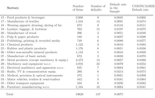
Sectors Number of firms Number of defaults Default rate in the Sample UNIONCAMERE Default rate 15 - Food products & beverages 2,008 9 0.0045 0.0302 17 - Manufacture of textiles 1,544 14 0.0091 0.0474 18 - Wearing apparel; dressing; dyeing of fur 673 9 0.0134 0.0511 19 - Leather; luggage, & footwear 762 15 0.0197 0.0375 20 - Manufacture of wood 396 2 0.0051 0.0249 21 - Pulp & paper products 540 2 0.0037 0.0298 22 - Publishing, printing & recorded media 749 6 0.0080 0.0377 24 - Chemical products 1,122 2 0.0018 0.0383 25 - Rubber and plastic products 1,176 6 0.0051 0.0338 26 - Other non-metallic mineral products 1,142 5 0.0044 0.0309 27 - Manufacture of basic metals 672 2 0.0030 0.0378 28 - Metal products (except machinery & equip.) 2,473 14 0.0057 0.0280 29 - Machinery and equipment n.e.c. 2,916 23 0.0079 0.0352 31 - Electrical machinery and apparatus n.e.c. 835 7 0.0084 0.0361 32 - Radio, TV & communication equip. 280 6 0.0214 0.0473 33 - Medical, precision & optical instruments 472 1 0.0021 0.0399 34 - Motor vehicles, trailers & semi-trailers 442 8 0.0181 0.0364 35 - Other transport equipment 234 6 0.0256 0.0382 36 - Furniture; manufacturing n.e.c. 1,184 10 0.0084 0.0341
Total 19628 147 0.0075
Table 1: The first three columns report respectively the number of firms, the number of defaults default rates in the sample, computed at 2-Digit sectoral level. The last column displays the corresponding default rates in the population of Italian limited liability firms (averages between 2003 and 2004 – Source: the association of the Italian Chambers of Commerce, UNIONCAMERE).
at the population level.
In the present work we use a set of financial and economic variables derived from CeBi balance sheet data. On the financial side, although we can build less indicators than one typically finds in studies of bankruptcy prediction, we can anyway capture the “strands of in-tuition” (see Carey and Hrycay, 2001) lying behind this type of analysis using three variables: Interest Expenses (IE), which provides a flow measure of the annual costs bore by firms to repay debt; Leverage, which is a standard indicator of the relative balance between external vs internal financing; and, finally, the Financial-Debt-to-Sales ratio (FD/S), which gives a stock measure of overall exposure, scaled by the size of the firm. To cure the potential problems arising from the limited number of financial variables we will perform robustness checks aug-menting our models with an official rating index provided by CeBi. Rating procedures are indeed designed to embrace a wider range of firms’ characteristics, together with qualitative and quantitative assessment of industry as well as national scenarios, technological changes, regulatory framework, and so on.12 The CeBi index is a “issuer credit rating”, meaning that it
gives an assessment of the obligor’s overall capacity to meet its obligations, without implying any specific judgment about the quality of a particular liability of the company. It is updated
12
This is typically the case with credit ratings issued by international agencies (see the “prototype risk rating system” described in Crouhy et al., 2001). This tendency has been more recently confirmed, by the effect of the provisions of the Basel II process, encouraging banks and financial institutions to also introduce ratings-based internal systems of risk assessment which consider a broad and multidimensional evaluation of their exposure (see BIS, 2001).
at the end of each year, and thus allowed to change over time. The method employed for the computation of the index is exclusive property of CeBi. There is, however, no reason to expect that the procedure is dramatically different from the methods applied by other rating agencies, both in terms of being targeted over the very short run (as said, one year ahead) and in terms of embracing a wide range of firms’ characteristics. Finally as a further measure of firm overall financial soundness, we will consider a proxy of the Distance to Default (DD) measure. Distance to Default is at the core of the last generation of empirical models of default prediction, adopted both by scholars and practitioners.13 The theoretical foundation of this
measure derives from an application of classical finance theory (Black and Scholes, 1973; Mer-ton, 1974), modeling the market value of firm equity as a call option on the value of the firm, with strike price given by the face value of its liabilities. DD is defined as a function of firms’ underlying value of assets, of the volatility of the latter and of the face value of debt. Under standard assumptions, the probability of default is obtained as the value of a standardized Normal density computed in DD, which is therefore a sufficient statistic to predict default.
Concerning economic characteristics, we are able to include in the analysis measures of size, growth, profitability and productivity, that is, the four basic levels which theoretical models as well as empirical research in industrial economics suggest to capture the crucial measures of firm performances. Several proxies can be in principle adopted to measure each of these dimensions, each proxy capturing complementary aspects of the same phenomenon. First, concerning firm size, revenue based (sales or value added) measures appear to be more suited to have a relationship with default than alternative “physical” (in terms of employment or capital) measures. Thus, we measure size in terms of Total Sales (S), and, accordingly, the growth rate of Total Sales (gS) is used to measure firm growth. Second, concerning profitability,
we want a proxy of the margins generated by the industrial or operational activities of the firms, which is the level we are interested into, avoiding definitions of income or profits influenced by financial strategies and taxation. Accordingly, we define profitability in terms of the return on sales (ROS), i.e. the ratio between Gross Operating Income and Total Sales. Finally, productive efficiency is captured by a standard index of labor productivity, measured in terms of value added per employee. Using labor productivity and gross operating income we are focusing on the more operative part of firm activity. We have no access to the kind of data typically used to estimate the stock of productive capital (like tangible assets). Consider however that while the cost and age of capital endowments certainly play a role in defining firm productive capabilities, their cumulative effect is already reflected in the financial variables we are considering.14
3
Descriptive analysis
This section analyzes if and to what extent the economic and financial characteristics of defaulting firms differ from the rest of the sample. We compare the empirical distribution of the relevant variables across the two groups of firms. Notice that the estimates of kernel densities provide information on properties of the variables, such as shape, degrees of heterogeneity among different classes of firms, skewness, etc., which are usually ignored by financial studies
13
See Duffie et al. (2007), for the most recent advance in financial literature, and the works cited therein for a review of duration models based on Distance to Default. Crosbie and Bohn (2003) offer an extensive introduction to Moody’s KMV model, which is also based on Distance to Default theory.
14
The short horizon of our analysis implies that capital intensity of each firm is basically fixed over the sample period.
0.001 0.01 0.1 7 8 9 10 11 12 13 14 log(Pr) log(S) Non Default - 1998 Default - 1998 0.001 0.01 0.1 7 8 9 10 11 12 13 14 log(Pr) log(S) Non Default - 2002 Default - 2002
Figure 1: Empirical density of Total Sales (S) in 1998 (left) and 2002 (right): Defaulting vs Non-Defaulting firms.
specialized in default prediction. To take account of the possible intertemporal variation, we present results at different time distance to default, comparing densities in the first available year, 1998, with densities obtained in the last year before default occurs, 2002. We apply non-parametric techniques, which do not impose any a priori structure to the data, thereby allowing to take a fresh look at the heterogeneities possibly existing both within and across the two groups of firms. The descriptive nature of this analysis is supplemented by formal statistical tests for distributional equality, performed in the next Section.
3.1
Economic characteristics
We start with the comparison of firm size. In the two panels of Figure 1 we plot, on a double logarithmic scale, the kernel density of firm size (S) estimated for defaulting and non-defaulting firms in 1998 and in 2002. The actual values of S for each defaulting firm are depicted in the bottom part of each plot.15
First look at 1998. Somewhat contrary to what one might conjecture, defaulting firms are neither less heterogeneous nor smaller with respect to the rest of the sample. The two densities are indeed very similar: supports are comparable, and the shapes are both right-skewed, an empirical result repeatedly found in the literature on firm size distribution. Actually, the right part of defaulting firms density suggests that default events are more frequent among medium-big sized firms rather than at small sizes. Estimates for 2002, in the right panel, show that these properties remain stable over time, as the default is approaching. The upper tail of the defaulting firms’ distribution is indeed even heavier as compared to 1998. A formal non-parametric test of multi-modality (Silverman, 1986) cannot reject the presence of bimodality in the distributions of defaulting firms (with a p-score of 0.72 for 1998 and of 0.63 for 2002). Such differences in the tail behavior are anyhow due to relatively few very big firms (see the dots at the bottom of the plots). Instead, in the central part of the densities, where most of the observations are placed, the overlap is almost perfect. Overall, the evidence is therefore suggestive that there is no clearcut relationship between size and the event of default:
15
Here, as well as in the following, estimates are performed applying an Epanenchnikov kernel, and the bandwidth is set following the “optimal rules” suggested in Silverman (1986), Section 3.4.
0.001 0.01 0.1 1 -1 -0.5 0 0.5 1 1.5 2 2.5 3 log(Pr) gS Non Default - 1999 Default - 1999 0.001 0.01 0.1 1 -1 -0.5 0 0.5 1 1.5 2 2.5 log(Pr) gS Non Default - 2002 Default - 2002
Figure 2: Empirical density of Total Sales Growth (gS) in 1999 (left) and 2002 (right):
Defaulting vs Non-Defaulting firms.
operating above a certain size threshold does not seem to provide any relevant warranty in preventing default.
Next we focus on firms’ growth. Figure 2 shows kernel densities of Total Sales growth rates, gS, for defaulting and non-defaulting firms. Given the initial year of the sample is 1998,
the first available data point is for 1999. This is shown in the left panel, while 2002 is depicted on the right graph. As before, actual values of gS for defaulting firms are reported below the
estimated densities.
Defaulting firms do not appear to significantly differ from the rest of the sample when considering the portions of supports where most of the probability mass is concentrated (ap-proximately between −0.5 and 0.5). In this interval, the distributions are crossing each other, and the estimated shapes are very similar, independently from the different time distance to default considered. One difference emerges regarding the variability of growth episodes: in 2002, that is closer to the default event, the width of the supports spanned by the defaulting group is sensibly narrower, especially in the right part of the support. This gets also mirrored in the tails (outside the interval [−0.5, 0.5]), where we however observe some differences across the two groups. In both years considered, left tail behavior is similar across the two groups, suggesting similar occurrence of extremely bad growth records. Conversely, only few default-ing firms are responsible for the peaks present at the top extremes. The different sizes of the two compared samples is likely to play a role in this respect. Similarly to what noted for size, however, these tail patterns concern a very low number of firms, and therefore they offer too weak evidence to conclude that one of the two groups is significantly outperforming the other. We then repeat the same exercise with profitability performance. Figure 3 reports kernel estimates of ROS densities in 1998 and 2002. The two groups of firms tend this time to differ, as defaulting firms perform clearly worse than the rest of the sample, especially for positive values of ROS. In 1998, the two distributions are substantially overlapping in the negative half of the support, while the density of defaulting firms lies constantly below that of the other group in the positive half. The same ranking gets reinforced in 2002. The distance between the two distributions in the right part of the support increases, and the density of defaulting firms is much concentrated at negative values. Despite negative performance is experienced also by non-defaulting firms, the evidence suggests that a sort of selection on profitability is at work: default events tend to be associated with lower profitability levels. In addition, time
0.01 0.1 1 10 -0.4 -0.2 0 0.2 0.4 log(Pr) ROS Non Default - 1998 Default - 1998 0.01 0.1 1 10 -0.4 -0.2 0 0.2 0.4 log(Pr) ROS Non Default - 2002 Default - 2002
Figure 3: Empirical density of Profitability (ROS) in 1998 (left) and 2002 (right): Defaulting vs Non Defaulting Firms.
0.01 0.1 1 2 3 4 5 6 log(Pr) log(VA/L) Non Default - 1998 Default - 1998 0.01 0.1 1 1 2 3 4 5 6 7 log(Pr) log(VA/L) Non Default - 2002 Default - 2002
Figure 4: Empirical density of Labour Productivity (VA/L) in 1998 (left) and 2002 (right): Defaulting vs Non Defaulting firms.
plays an important role in the story, since profitability differentials across the two groups tend to become wider in the very short run before default.
Finally, the densities of Labour Productivity, plotted in Figure 4, show that a similar mechanism is also acting upon productive efficiency. The estimates obtained for non-defaulting firms tend indeed to lie above the ones obtained for defaulting firms in the right part of the supports, especially if one nets out the effect of few outliers present at the extremes. The intertemporal patterns also resembles the findings observed for profitability: the productivity advantage of non-defaulting firms increases over time. This suggests that Labour Productivity too represents a discriminatory factor telling apart defaulting firms from the rest of the sample. The relevance of this factor seems increasing as the default event approaches.
3.2
Financial characteristics
We then ask if defaulting firms display any significant peculiarity in terms of the financial variables considered in the analysis.
0.001 0.01 0.1 1 -10 -9 -8 -7 -6 -5 -4 -3 -2 -1 log(Pr) log(IE/S) Non Default - 1998 Default - 1998 0.001 0.01 0.1 1 -10 -9 -8 -7 -6 -5 -4 -3 -2 -1 log(Pr) log(IE/S) Non Default - 2002 Default - 2002
Figure 5: Empirical density of Interest Expenses scaled by size (IE/S) in 1998 (left) and 2002 (right): Defaulting vs Non-Defaulting firms.
0.001 0.01 0.1 1 0 1 2 3 4 5 6 log(Pr) log(LEV) Non Default - 1998 Default - 1998 0.001 0.01 0.1 1 0 1 2 3 4 5 6 7 log(Pr) log(LEV) Non Default - 2002 Default - 2002
Figure 6: Empirical density of Leverage (LEV) in 1998 (left) and 2002 (right): Defaulting vs Non-Defaulting firms .
Figure 5 shows densities of Interest Expenses over Sales IE/S, i.e. the proportion of annual revenues that goes to meet interest payments. The resulting estimates, reported in logs, suggest a clearcut difference between defaulting and non-defaulting firms. Both the average and the modal values of the former group are indeed larger than the ones of the latter. Also the shape of the distributions differ, with the defaulting firms much more concentrated in the right part of the support. A further noticeable feature is that, whereas the estimates for non-defaulting firms do not change over time, the density of defaulting firms displays a right-ward shift of probability mass between 1998 and 2002. This means that the flows of interest payments per unit of output sold becomes heavier as the default event approaches.
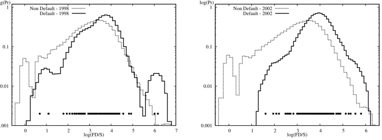
The densities of Leverage (Figure 6) and Financial Debt-to-Sales ratio (Figure 7) follow similar inter-temporal dynamics. The rightward shift in the Leverage distribution of defaulting firms indicates that the ratio between external vs. own resources increases over time, resulting into a disproportionate financial structure in proximity of the default event. At the same time, the even more remarkable shift in the FD/S ratio complement the above results on IE/S:
0.001 0.01 0.1 1 0 1 2 3 4 5 6 7 log(Pr) log(FD/S) Non Default - 1998 Default - 1998 0.001 0.01 0.1 1 0 1 2 3 4 5 6 log(Pr) log(FD/S) Non Default - 2002 Default - 2002
Figure 7: Empirical density of Debt-to-Sales ratio (FD/S) in 1998 (left) and 2002 (right): Defaulting vs Non-Defaulting firms.
not only the flow of debt repayment, but also the stock of debt is increasing when default approaches. Also notice that the differences between defaulting and non-defaulting firms, in terms of both Leveraged and FD/S ratios, are smaller than in terms of IE/S. This possibly signals that cost of debt is the financial factor which more sharply distinguish defaulters from non-defaulters.
4
Non-parametric inferential analysis
In order to add statistical precision to the comparison between the two groups of firms, we now perform formal tests of distributional equality. A range of testing procedures is in prin-ciple available. There are however some specific features of our data which must be carefully considered in selecting the most appropriate alternative. First of all, default events are much less frequent than non-defaults, and therefore we need a test which can be applied in the case of two uneven samples. Second, as shown in the previous section, the distributions we are going to compare display clear non-normalities and unequal variances, suggesting that non-parametric tests should be preferred over parametric ones. Further, even within the class of non-parametric tests for comparison of uneven samples, a common feature is to implicitly assume that the samples to be compared only differ for a shift of location, while their distribu-tions possess identical shapes. Given that equality of shapes is generally violated by our data, as shown by kernel densities, it is appropriate to employ tests which abandon this hypothesis. When distributions with different shapes are compared, looking at the relative location of medians, modes or means might no longer be very informative, as the very meaning of these measures changes with the nature of the underlying distribution. In this case a better measure of the relative position of the two samples is provided by the idea of stochastic (in)equality.16
Let FD and FN D be the distributions of a given economic or financial variable, for the
two samples respectively. Denote with XD ∼ FD and XN D ∼ FN D the associated random
variables, and with XD and XN D two respective realizations. The distribution FD is said to
16
As a robustness check we also performed the Wilcoxon-Mann-Witney (WMW) test, which is standard way to assess equality of medians under the assumption of equal shapes. Results were consistent with the evidence presented below.
Test of Stochastic Equality Variable Test 1998 1999 2000 2001 2002 IE/S FP stat 7.510 9.269 13.019 17.903 24.069 p-value 0.000 0.000 0.000 0.000 0.000 LEV FP stat 8.029 10.483 12.066 13.520 15.190 p-value 0.000 0.000 0.000 0.000 0.000 FD/S FP stat 7.490 10.480 14.387 16.037 17.229 p-value 0.000 0.000 0.000 0.000 0.000 TS FP stat 0.364 1.555 3.988 3.466 2.426 p-value 0.716 0.120 0.000 0.000 0.015 GROWTH FP stat 0.905 -0.618 -1.133 -3.927 p-value 0.365 0.536 0.257 0.000 PROF FP stat -4.609 -7.169 -7.186 -7.466 -11.176 p-value 0.000 0.000 0.000 0.000 0.000 PROD FP stat -5.310 -7.156 -7.167 -6.842 -8.855 p-value 0.000 0.000 0.000 0.000 0.000
Table 2: Fligner-Policello Test of stochastic equality, Defaulting vs Non-Defaulting firms. Observed value of the statistic (FP) and associated p-value. Rejection of the null means that the two distributions are different in probability. Rejection at 5% confidence level highlighted with bold.
dominate FN D if Prob{XD > XN D} > 1/2. That is, if one randomly selects two firms, one
from the D group and one from the ND group, the probability that the latter displays a smaller value of X is more than 1/2, or, in other terms, it has a higher probability to have the smaller value. Now, since
Prob{XD > XN D} =
Z
dFD(X) FN D(X) , (1)
a statistical procedure to assess which of the two distributions dominates can be formulated as a test of H0 : Z dFDFN D = 1 2 vs H1 : Z dFDFN D 6= 1 2 . (2)
The quantity ˆU proposed in Fligner and Policello (1981) provides a valid statistic for H0. We
apply their procedure exploiting the fact that, in case of rejection of the null, the sign of the Fligner-Policello (FP) statistic tells which of the two group is dominant: a negative (positive) sign means that defaulting (non-defaulting) firms have a higher probability to take on smaller values of a given financial or economic variable.17
Table 2 presents the results obtained year by year. The high rate of rejection of H0
supports the evidence provided by the previous descriptive analysis, confirming that the two groups differ under many respects. First, looking at financial variables, the signs of the FP statistics are consistent with the idea that defaulting firms present weaker performances than non-defaulters, under all the dimensions considered. Second, as far as economic variables are
17
Under the further assumption that the two compared distributions are symmetric, testing H0is equivalent
to testing for equality of medians between possibly heteroskedastic samples. This is what is usually referred to as the Fligner-Policello test.
concerned, defaulting firms tend to be less profitable and less productive than those in the other group, and we tend to confirm that, possibly due to the already mentioned tail behavior observed in the empirical distribution of Total Sales, defaulting firms are comparatively bigger. Growth rates instead display statistically significant differences in 2002 only.
Overall, the findings broadly confirm the conclusions based on the kernel estimates. Notice also that differences in both economic and financial performances matter over both the shorter and the longer run. With the exception of growth, the null is already rejected at the beginning of the period, or at least some years before default.
5
Robust probit analysis of default probabilities
The analyses conducted so far tell us how defaulting firms compare with non-defaulting firms when each economic or financial dimension is considered on its own. In this section we try to identify which are the main determinants of default once the effects of economic and financial factors are allowed to simultaneously interplay.
To this end, we frame our research questions so as to single out the effects of financial and economic variables within a more standard parametric setting. The response probability of observing the default event is modeled as a binary outcome Y (taking value 1 if default occurs, 0 otherwise), and then estimated conditional upon a set X of explanatory variables and controls. We employ a probit model, where the default probability is assumed to depend upon the covariates X only through a linear combination of the latter, Xβ, which is in turn mapped into the response probability through
Prob (Y = 1 | X) = Φ(Xβ) , (3) where Φ(·) is the cumulative distribution function of a standard normal variable, with associ-ated density φ(·).
Several variations of equation (3) are explored in the following, including different sets of regressors. The estimation strategy is however common to all the specifications, and is intended to solve the under-weighting of default events in our data, as compared to distress rates observed in the reference population of Italian limited liability firms (recall Table 1). As anticipated, this feature of the dataset is dangerous for regression analysis, since it might give rise to a classical “choice-based sample” bias (Manski and McFadden, 1981), a well known problem in studies of default probability since Zmijevski (1984). There exist different methods to get rid of the potential bias, either by employing specific estimators designed for this situation (see Manski and Lerman, 1977; Imbens, 1992; Cosslet, 1993), or by performing bootstrap sampling. We follow this second alternative, which has the advantage that it does not depend on specific assumptions about the distribution of the estimated parameters. The only requirement is that each bootstrap sample needs to be representative of the population, and the way this is achieved is explained in the following. Studies of distress prediction, where oversampling of default events is the typical situation, achieve this goal by performing randomized re-sampling of both defaulting and non defaulting firms in the desired, population-wide proportions (see, for instance Grunert et al., 2005). In our case, the relatively low number of defaults available in the data suggests to take defaulting firms fixed, and randomly extract a subset of non-defaulting firms only. This is the strategy we apply in the following. In particular, in order to reduce the bias as much as possible, sampling of non-defaulting firms is implemented with replacement within each 2-Digit industry, so that the ratio of defaulting over non-defaulting firms equals the population-wide default frequency reported in Table 1
at this level of sectoral aggregation. The sampling procedure is repeated several times, and estimates of the different specifications of equation (3) are repeated on the sample obtained at each round. Averaging over the number of runs then yields robust estimates. We will present results based on 200 independent replications, which turned out to be a large enough bootstrap sample to achieve convergence in the estimated coefficients.
One problem remaining out of our direct control concerns the fact, due to the way data are collected, some of the firms treated as non-defaulters could in fact be defaulting firms. Two considerations are due here. On the one hand, the possible presence of defaulting into our control group of non-defaulters implies that, whenever a variable has a statistically different effect between the two groups, the “true” difference would be even more significant if we could precisely identify non-defaulters. Thus, we can safely comment on our results when a variable turns significant.18 On the other hand, it could be that variables that do not appear to have
significantly different effects between the two groups, have indeed different effects, but such differences have been made invisible by the presence of defaulting firms in the control group. Here is where our re-sampling scheme really helps. Indeed, remember that defaults occur with low frequency in the reference population (c.f. Table 1). Therefore, the probability to have a defaulter in the control group must be very small, and Monte Carlo methods are well known to be robust with respect to this kind of disturbance. So even the occurrence of this second problem can be considered remote.
Our main goal is to test the commonly held presumption that default is mainly determined by poor financial conditions, especially in the short run before default occurs. Thus, our choice of the specifications of equation (3) is primarily meant to verify whether adding economic variables, in general, and looking at their effect at different time distances to default, in particular, might improve the chance to correctly distinguish “healthy” firms from those at risk of default. Our conjecture is that explicit consideration of economic variables should improve the understanding of default dynamics.
Accordingly, we focus on comparing results of two main specifications. The first model includes, among the regressors, only financial indicators, together with a full set of sectoral (2-Digit) control dummies
Prob (YT = 1 | Xt) = Φ(β0t+ β1t IEt St + β2t LEVt+ β3t F Dt St + δtSectort) , (4)
where, as in the previous sections, IE/S stands for Interest Expenses scaled by Total Sales S, LEV is Leverage, and FD/S is the Financial-Debt-to-Sales ratio. In the second specification we then add the economic variables
Prob (YT = 1 | Xt) = Φ(β0t+ β1t IEt St + β2t LEVt+ β3t F Dt St + β4t ln St+ (5)
β5t P RODt+ β6tP ROFt+ β7tGROW T Ht+ δtSectort) ,
where S is size (again in terms of Total Sales), PROD is Labour Productivity (as Value Added per employee), PROF is profitability (in terms of Return on Sales), and GROWTH
18
This is standard in controlled experiments. Consider for instance that you want to test if a given drug is effective. You treat a group of people for one month and then compare the result with an untreated group. Suppose you find significant differences, and therefore conclude that the drug is actually effective. Now if somebody in the control group had some doses of the drug, this of course testify in favour of the effectiveness of the drug, not against it: those control subjects who were not in contact with the drug were different enough to suggest an effective treatment. Coming back to our problem: if we find significant differences comparing the characteristics of defaulters and the control group of non-defaulters, then these differences would be even more significant if we could eliminate defaulters from the control group.
is the log-difference of Total Sales. Recall that, due to the characteristics of the dataset, the covariates can be measured over the different years of the window 1999-2002, while the default/non default event Y is only measured at the end of the period (at time labeled as T ).19. Thus, comparing estimates in the different years allows to capture the dynamic effects
of the covariates on the probability of default at different time distances to the default event. This is a relevant issue, especially in understanding the extent to which financial conditions are indeed capturing the past history of economic dimensions of firm performance.
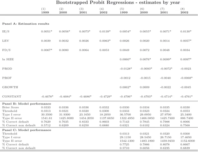
In Panel A of Table 3 we show results obtained in each year, averaging over the 200 bootstrap replications. Columns 1-4 concern estimates of model (4) while Columns 5-8 refer to the probit specification in (5). Notice that all models are estimated taking z-scores of the covariates. This reduces them to have equal (zero) mean and equal (unitary) variance, allowing for a direct comparison of the magnitudes of the estimated effects across different models. We report marginal effects, computed as standard in the sample mean of the covariates, which is zero given z-scoring. Statistical significance is assessed through confidence intervals based on bootstrap percentiles (see Efron and Tibshirani, 1993). That is, we first estimate the empirical probability distribution function (EDF) of the 200 coefficients obtained over the bootstrap runs. Then, statistical significance at the α% level is rejected if the zero falls within an interval
[ˆq(α/2), ˆq(1 − α/2)] , (6) where ˆq(α) stands for the estimate of α-th quantile of the bootstrap distribution estimated from the EDF.20 Estimates of sectoral dummies are not reported, as we indeed find that only
less than 5% of these coefficients turns statistically significant at the 5% confidence level. Moreover, the few significant sectors tend to differ across the different exercises considered. These results yield strong support that sectoral specificities do not affect the link between the probability of default and the set of economic and financial characteristics included in our analysis.
The estimates corresponding to the “financial variable only” equation (4) show that cost of debt is the most relevant financial dimension. We indeed find that the relatively big and positive effect of IE/S is significant over the entire period, while Leverage and FD/S display weaker significance. This relates to the interesting variation over time of the estimates. The stock of debt tends indeed to be more relevant at longer distance to default, then loosing significance in the shorter run, when the estimated impact of the IE/S increase remarkably. Notice also that Leverage is turning significant only in the last year before default. This possibly captures part of the short run effect played by an excessive debt burden, thereby compensating for the disappearing significance of FD/S.
The findings in the right part of the table, obtained from specification (5), confirms the predominant role played by cost of debt among the financial indicators, but also offer strong support to the idea that economic characteristics of firms have a relevant effect, additional to that of financial variables. Concerning their sign, the effects, when significant, are consis-tent with the foregoing evidence on kernel densities and stochastic dominance, discussed in Section 3 and Section 4. Size and Growth have indeed a positive effect, while Productivity
19
Once again, 1998 is excluded simply because growth rates cannot be computed for that year.
20
Several refinements of the bootstrap estimates of confidence intervals are discussed in the literature, most notably the BCa and ABC corrections. These methods require an estimate of the bias, which we can only
obtain by performing a “first step” probit regression on the overall original sample. This is however exactly what we want to avoid, in order to overcome under-sampling of defaulting firms. Alternatively, one could try to estimate the bias by re-sampling from each random sample. This second order bootstrap seems to us unnecessary due to the relatively large size of the sample considered.
Bootstrapped Probit Regressions - estimates by year
(1) (2) (3) (4) (5) (6) (7) (8)
1999 2000 2001 2002 1999 2000 2001 2002
Panel A: Estimation results
IE/S 0.0051* 0.0056* 0.0073* 0.0139* 0.0054* 0.0055* 0.0071* 0.0130* LEV 0.0039 0.0032 0.0026 0.0063* 0.0026 0.0020 0.0014 0.0057* FD/S 0.0067* 0.0080 0.0064 0.0053 0.0049 0.0072 0.0048 0.0034 ln SIZE 0.0060* 0.0076* 0.0099* 0.0097* PROD -0.0128* -0.0093* -0.0072* -0.0023 PROF -0.0012 -0.0015 -0.0040 -0.0068* GROWTH 0.0062* 0.0009 -0.0022 -0.0045 CONSTANT -0.4678* -0.4684* -0.4686* -0.4729* -0.4706* -0.4703* -0.4714* -0.4761*
Panel B: Model performance
Brier Score 0.0333 0.0336 0.0336 0.0332 0.0330 0.0334 0.0335 0.0330
Threshold 0.0313 0.0321 0.0320 0.0300 0.0333 0.0323 0.0324 0.0353
Type I error 30.3500 31.9300 23.1650 18.2950 36.5700 29.0950 27.9700 25.3400
Type II error 1541.61 1425.8000 1454.2050 1137.6650 1322.4950 1466.0850 1425.7400 886.7400
% Correct default 0.7629 0.7635 0.8333 0.8603 0.7143 0.7845 0.7988 0.8066
% Correct non default 0.5712 0.6209 0.6250 0.6880 0.6321 0.6102 0.6324 0.7568
Panel C: Model performance
Threshold 0.0313 0.0321 0.0320 0.0300
Type I error 29.1150 28.5450 26.7150 17.4650
Type II error 1542.1300 1483.1800 1459.9450 1152.6000
% Correct default 0.7725 0.7886 0.8078 0.8667
% Correct non default 0.5710 0.6056 0.6235 0.6839
Table 3: Probit estimates of default probabilities as modeled in Eq. (4) and Eq. (5) – results over 200 bootstrap replications. Variables are in z-scores. Panel A: Bootstrap means of marginal effects at the sample average of covariates, * Significant at 1% level. Panel B-C: Bootstrap means of model performance measures.
and Profitability reduce the probability of default. Also notice intertemporal variation of the effects, revealed by varying magnitude of estimates, together with patterns of significance. In particular, Size is strongly significant in all years and the effect seems increasing over time. The marginal effect of Productivity is instead decreasing over time, and looses its significance in the last year. There might be an interaction with Profitability, which indeed turns sig-nificant, and with a relatively big negative coefficient, in 2002, possibly “absorbing” part of the loosing significance of Productivity in this same year. The role of Growth seems instead marginal, with a moderate effect significant only in the first year.
Overall, we can conclude that statistical relevance of economic variables is preserved even at very short time distance to default. Financial and economic dimensions of firm operation, in other words, both matter at longer as well as at shorter run. This suggests existence of strong capital market imperfections, preventing to consider financial structure of firms as em-bedding all the relevant information on the probability that a firm incur default. Rather, industrial characteristics and performances capture important and complementary determi-nants of default, even in the short run. The bootstrap procedure, with its random sampling of firms, allows to safely conclude that the observed intertemporal variation cannot be simply attributed to outliers or missing observations affecting the estimates in each specific year.21
21
A further test of the contribution offered by economic variables is conducted in Panel B of the same Table 3, where we focus on goodness of fit and prediction accuracy of the models.
The first measure adopted is the Brier Score (Brier, 1950), a standard indicator employed in the literature to assess the relative explanatory power of alternative models of distress prediction. For each firm i, this is computed as 1/NPN
i=1(Yi− Pi)2, where N is the number
of firms, Pi is the estimated probability of default of firm i based on coefficient estimates of
the probit regressions, and Yi is the actual realization of Y for firm i, default (Yi = 1) or
non-default (Yi = 0). We report the bootstrap mean of this measure over the 200 replications.
Of course, the lower the Brier Score, and the higher the performance of the model. Thus, comparisons of results between corresponding specifications – i.e. looking at each “financial variables only” model vs. the “financial plus economic variables” model estimated in the same year – strongly confirm that inclusion of economic variables provides an improved model performance in all years.
Prediction accuracy of the models is then evaluated building upon the concept of correctly classified observations. This is based on the idea of classifying a firm as defaulted (assigning Y = 1) whenever its estimated probability of default, Pi, is bigger than a certain threshold
value τ , while a firm is classified as non-defaulting otherwise (assigning Y = 0). Such a classification will in general differ from the true default or non-default status. A Type I error is defined as the case when a firm which is actually defaulting (a true Yi=1 in the data)
is classified as non-defaulting, and thus is assigned a 0. A Type II error is instead counted when a non-defaulting firm (a true Yi=0) is assigned a 1 by the classification procedure.
Correspondingly, the percentage of correctly predicted 1’s (“% Correct default” in the Table) gives the ratio of the correctly predicted defaults over the actual number of defaults in the sample. Conversely, the percentage of correctly predicted 0’s (“% Correct non default” in the Table) gives the fraction of correctly classified non-defaulting firms over the actual number of non-defaulters. Within this set of measures, it is standard to prefer models reducing Type I errors (or maximizing the percentage of correctly predicted defaults). Indeed, from the point of view of an investor, failing to predict a bankruptcy (and investing) might be much more costly than mistakenly predicting a default (and not investing).
Quite obviously, the degree of prediction accuracy depends on the specific value of the threshold τ . Different criteria are in principle available to set this value. We consider an “optimal” τ∗
so as to minimize the overall number of prediction errors (Type I plus Type II), weighted by the relative frequency of zeros and ones. This is obtained in practice by solving the following minimization problem
τ∗ = arg min τ 1 N0 X i∈N D Θ(Pi− τ) + 1 N1 X i∈D Θ(τ − Pi) ! , (7)
where Θ(x) is the Heaviside step function, taking value Θ(x) = 0 if x < 0 and Θ(x) = 1 if x > 0, while N0 and N1 stand for the actual number of non-defaulting and defaulting firms in
our sample, respectively, with ND and D the two corresponding sets.22
We repeat the minimization procedure for each bootstrap replication, and then compute Type I and Type II errors, together with the percentage of correctly predicted default and
and do not change if we take the number of employees as a proxy for size.
22
Minimizing the overall number of errors is equivalent to maximizing the total sum of correctly predicted observations. The weighting is instead introduced to address the specific characteristics of our exercise. True 0’s are indeed much more frequent than true 1’s, simply because default rates in each bootstrapped sample equal the population-wide frequencies presented in Table 1.
non default events. In Panel B we report averages of these measures computed over the 200 bootstrap replications, together with the average value of the optimal threshold found at each run.23
Results suggests that the models including economic variables tend to produce more Type I errors (and thus lower number of Type II errors) as compared to corresponding “financial vari-ables only” specifications. It is however important to underline that a direct comparison of these numbers is not truly informative, as they are obtained with different values of τ∗
, each optimal for its own model. A much more meaningful comparison between two models would instead require to evaluate the performance of one model under the optimal threshold of the other model. This is done in Panel C of the same Table 3. Here prediction accuracy of the “financial plus economic variables” specifications are computed taking the optimal threshold τ∗ of the “financial variables only” model estimated in the same year: if the former performs
better under the τ∗
of the latter, this would imply a strong confirmation that including eco-nomic variables into the analysis is improving predictive power with respect to the benchmark “financial variables only” specification. What we observe is that, compared to the benchmarks figures of Panel B, the models including economic variables perform better in terms of Type I errors (and correctly classified defaults), in all the years but 2001. This offer further evidence that, consistently with suggestions derived from Brier Scores, the contribution of economic variables is important. Once again, the improved performance in 2002 confirms that this holds true even in the very proximity of the default event.
6
Distance to Default and credit rating
Following the literature on corporate default prediction, there are two further measures which one should consider in the analysis of default probability, Distance to Default and credit ratings.
Despite theoretically appealing, DD has two major limitations. First, due to the non trivial procedures required to get a numerical solution of the models, computation of the measure is in practice rather complicated. Second DD applies to publicly traded firms only, because the the underlying market value of a firm, not observable in practice, is estimated using market value of equity, essentially exploiting the standard hypothesis that markets are fully informed and stock prices instantaneously incorporate all the relevant information. A solution to the first problem is to adopt a “naive” DD measure (Bharath and Shumway, 2008), which is much easier to compute than the original DD and ensures, at the same time, equivalent results in terms of default prediction accuracy. Yet, the naive DD still requires data on market values of firms’ equity and assets, so that it is not obvious how it is possible to include this measure in the context of our study, where the scope of analysis goes beyond the limited subset of publicly traded firms, and, consequently, only accounting data are available. Nevertheless, motivated by the widespread use and the solid theoretical basis of DD, we attempt to include such a potentially important explanatory variable in the analysis. We start from the naive DD estimator of Bharath and Shumway (2008) and build an equivalent measure, denoted Book Distance to Default (Book DD), based on accounting data on value of shares and value of debt, which we can derive from available figures on Leverage and Total Assets. Notice that computations exploit time series means and volatility of these variables, and thus Book DD
23
The application of the bootstrap to compute model performance measures is particularly important. Zmijevski (1984) indeed shows that classification and prediction errors of the defaulting group are generally overstated without an appropriate treatment of the “choice-based sample” problem.
Bootstrap Probit with Distance to Default - estimates by year
Rating only Rating, Financial and Economic
(1) (2) (3) (4) (5) (6) (7) (8) 1999 2000 2001 2002 1999 2000 2001 2002 Panel A: Estimates IE/S 0.0074* 0.0066* 0.0086* 0.0090* LEV 0.0005 0.0015 0.0002 0.0029 FD/S 0.0024 0.0053 0.0021 0.0026 ln SIZE 0.0066* 0.0076* 0.0075* 0.0072* PROD -0.0097* -0.0067* -0.0041 -0.0010 PROF 0.0013 -0.0005 -0.0024 -0.0049* GROWTH 0.0053* 0.0004 -0.0019 -0.0020 Book DD -0.0210* -0.0204* -0.0898* -0.0816* -0.0164* -0.0147* -0.1095* -0.1064* CONSTANT -0.4698* -0.4693* -0.4764* -0.4766* -0.4733* -0.4726* -0.4800* -0.4811*
Panel B: Model performance
Brier Score 0.0332 0.0335 0.0335 0.0335 0.0329 0.0334 0.0333 0.0331
Threshold 0.0374 0.0385 0.0364 0.0362 0.0343 0.0315 0.0345 0.0361
Type I error 43.9900 51.6650 52.2200 49.2350 32.6450 22.6450 30.2400 29.2500
Type II error 1224.4550 1180.9650 1305.3200 1358.4750 1159.7000 1431.3350 1131.6050 901.6500
% Correct default 0.6364 0.5964 0.6014 0.6242 0.7302 0.8231 0.7692 0.7767
% Correct non default 0.6386 0.6677 0.6420 0.6274 0.6577 0.5973 0.6896 0.7527
Panel C: Comparisons of prediction performance against the “Rating only” model of the same year
Threshold 0.0374 0.0385 0.0364 0.0362
Type I error 41.6750 46.8650 34.7800 29.5750
Type II error 951.9550 974.0700 1020.3050 892.4400
% Correct default 0.6556 0.6339 0.7345 0.7742
% Correct non default 0.7190 0.7259 0.7202 0.7552
Table 4: Probit estimates of default probabilities by year, including Book DD as modeled in Eq. (8) and Eq. (9) – results over 200 bootstrap replications. Variables are in z-scores. Panel A: Bootstrap means of marginal effects at the sample average of covariates, * Significant at 1% level. Panel B-C: Bootstrap means of model performance measures.
takes a single value for each firm, not varying over time (see the Appendix for details on construction of the proxy).
We explore estimates of a first model where Book DD enters as the sole covariate
P (YT = 1 | Xt) = Φ(β0+ δ BookDD) , (8)
and then add the full set of financial and economic variables considered in this work
P (YT = 1 | Xt) = Φ(β0t+ δ BookDD + β1t IEt St + β2tLEVt+ β3t F Dt St + β4t St+ (9)
β5tP RODt+ β6t P ROFt+ β7t GROW T Ht) .
The estimation strategy goes exactly as in previous section.24
Results, in Table 4, are clearcut. We find that Book DD has a tight link with default: marginal effects are big and always statistically significant. However, the inclusion of this further regressor does not affect any of the results achieved in the foregoing section: in all the
24
years considered the sign, magnitude and patterns of statistical significance of the effects of financial and economic variables remain in practice unchanged as compared to our baseline results in Table 3. We only observe that Distance to Default absorbs Leverage and FD/S in some years, but this is not surprising as equity and debts enter the definition of Book DD. Moreover, the goodness of fit measures in Panel B show that the inclusion of Book DD does not produce any substantial improvement in the predictive ability of the model: Brier score and both types of error are indeed comparable with the ones reported in Table 3. In the same direction, Panel C shows that the inclusion of economic and financial variables yield predictions which are noticeably better that those obtained using only the Book DD measure. The second extension of the model we want to consider in this section includes official CeBi credit rating among the regressors. The credit rating is essentially a short-run forecast of default probability, hence its inclusion could help to validate the statistical consistence of the timing effects discovered so far. While the analysis is performed using the credit rating index developed by CeBi, our exercise could be in principle replicated taking credit ratings from international agencies, such as Moody’s or Standard & Poor’s indexes. However, a first obvious advantage of the CeBi ratings lies in that they are available for all the firms included in our dataset. On the contrary, international agencies are mainly concerned with bigger Italian firms, those having reached an international relevance, and/or listed on stock exchanges around the world. As a result, using credit files issued by well known rating institutions would bias the scope of analysis towards a sub-sample of firms, not fully representative of the Italian industrial system. Another peculiar characteristic of the CeBi index is that it is an official credit rating. Indeed, founded as an agency of the Bank of Italy in the early 80’s, CeBi has a long-standing tradition as an institutional player within the Italian financial system. Credit rating construction is one of the core activities within its institutional tasks of providing assistance in banking system supervision. Nowadays a private company, CeBi is still carrying out an institutional mandate, as the Italian member within the European Committee of Central Balance Sheet Data Offices (ECCBSO), operating in close relationships with Italian Statistical Office and the major commercial banks. These observations allow us to be confident that CeBi ratings are reliable and maintained up to international standards.
The firms included in the database, no matter whether defaulting or non-defaulting at the end of the period, are ranked with a score ranging from 1 to 9, in increasing order of default probability: 1 is attributed to highly solvable firms, while 9 identifies firms displaying a serious risk of default. Notice that the ranking is an ordinal one: firms rated as 9 are not implied to have 9 times the probability of going default as compared to firms rated with a 1.
For the purpose of the present section, we build three classes only, which we label Low Rate firms (having lower probability of default, with credit ratings 1-6), Mid Rate firms (rated 7) and High Rate firms (rated 8-9). The transition matrices among the three groups, displayed in Table 5, summarize the salient properties of the rating index in the sample. Over the longer-run transition (1998 to default year), the Low Rate class is very stable, while both Mid and High Rate firms display a sort of “reversion to the mean” property, i.e. they have a higher probability to jump back to better ratings, as compared to the likelihood of remaining in the same class. This gets reflected in the transition probability to end up defaulting (last column), which is higher for Mid Rate firms than for High Rate firms. Similar patterns persist in the short run transition (2002 to default year). The numbers on the diagonal suggest higher stability within-class, as compared to the longer-run transition. Yet, the “reversion to the mean” property – towards improved ratings – is still present, even in the High Rate group. Notice however that the short-run transition probabilities to default (last column) are more
Default year
Low Mid High Default
1 9 9 8 Low 0.8948 0.0824 0.0176 0.0052 Mid 0.5402 0.3651 0.0743 0.0204 High 0.4589 0.3290 0.1991 0.0130 2 0 0 2 Low 0.9308 0.0583 0.0077 0.0032 Mid 0.3375 0.5446 0.0986 0.0192 High 0.1499 0.3512 0.4754 0.0236
Table 5: Credit ratings transition matrices.
in accordance with what one would expect: probability of default increases as rating worsens. This confirms the presumption that credit ratings are much better predictors of default in the very short run than over a longer distance to the event. In turn, the fact that the CeBi index displays variation over time is important, allowing to test the time effects of financial and economic variables observed in the foregoing probit regressions.25
According to the classification in three rating classes, we build three dummy variables taking on value 1 when a firm is belonging to one of the classes, and zero otherwise. These are then employed in order to investigate if inclusion of different credit rating conditions is able to affect the conclusions drawn from the baseline year by year estimates presented in the previous section. That is, running separate regressions for each year over the 1999-2002 sample period, we first estimate a “rating only” specification
Prob (YT = 1 | Xt) = Φ(β0t+ δ1t LOWt+ δ2tMIDt+ δ3tHIGHt) , (10)
allowing to get an idea of the explanatory power of the CeBi index, and then compare results with a second model where financial and economic characteristics enter together with ratings themselves
Prob (YT = 1 | X) = Φ(β0t+ δ1t LOWt+ δ2t MIDt+ δ3t HIGHt+ (11)
β1t IEt St + β2t LEVt+ β3t F Dt St + β4t St+
β5tP RODt+ β6t P ROFt+ β7t GROW T Ht) .
Table 6 shows the results. Due to obvious collinearity between the rating dummies and the constant term, one dummy cannot be estimated. We present coefficient estimates of regressions where only the Low and Mid Rate class are considered.26
25
Notice that firms’ “ability” to improve their rating does not depend on the exit of better firms from the sample. The matrices are indeed computed taking all the firms which are still in the sample in the last year, when default is measured, and then tracing back their credit rating history. The findings reported in Bottazzi et al. (2008) show that a similar intertemporal behavior in the CeBi index is also appearing when a different division of firms into rating classes is chosen.
26
Once again, statistical irrelevance of sectoral dynamics motivate the exclusion of 2-Digit dummies from the models.