HAL Id: hal-02923974
https://hal.archives-ouvertes.fr/hal-02923974
Submitted on 28 Aug 2020
HAL is a multi-disciplinary open access
archive for the deposit and dissemination of
sci-entific research documents, whether they are
pub-lished or not. The documents may come from
teaching and research institutions in France or
abroad, or from public or private research centers.
L’archive ouverte pluridisciplinaire HAL, est
destinée au dépôt et à la diffusion de documents
scientifiques de niveau recherche, publiés ou non,
émanant des établissements d’enseignement et de
recherche français ou étrangers, des laboratoires
publics ou privés.
A one-year comprehensive chemical characterisation of
fine aerosol (PM<sub>2.5</sub>) at urban, suburban
and rural background sites in the region of Paris
(France)
M. Bressi, J. Sciare, V. Ghersi, N. Bonnaire, J. B. Nicolas, J.-E. Petit, S.
Moukhtar, A. Rosso, N. Mihalopoulos, A. Féron
To cite this version:
M. Bressi, J. Sciare, V. Ghersi, N. Bonnaire, J. B. Nicolas, et al.. A one-year comprehensive chemical
characterisation of fine aerosol (PM<sub>2.5</sub>) at urban, suburban and rural background sites
in the region of Paris (France). Atmospheric Chemistry and Physics, European Geosciences Union,
2013, 13 (15), pp.7825-7844. �10.5194/acp-13-7825-2013�. �hal-02923974�
Atmos. Chem. Phys., 13, 7825–7844, 2013 www.atmos-chem-phys.net/13/7825/2013/ doi:10.5194/acp-13-7825-2013
© Author(s) 2013. CC Attribution 3.0 License.
EGU Journal Logos (RGB)
Advances in
Geosciences
Open Access
Natural Hazards
and Earth System
Sciences
Open AccessAnnales
Geophysicae
Open AccessNonlinear Processes
in Geophysics
Open AccessAtmospheric
Chemistry
and Physics
Open AccessAtmospheric
Chemistry
and Physics
Open Access DiscussionsAtmospheric
Measurement
Techniques
Open AccessAtmospheric
Measurement
Techniques
Open Access DiscussionsBiogeosciences
Open Access Open Access
Biogeosciences
Discussions
Climate
of the Past
Open Access Open Access
Climate
of the Past
Discussions
Earth System
Dynamics
Open Access Open Access
Earth System
Dynamics
DiscussionsGeoscientific
Instrumentation
Methods and
Data Systems
Open Access
Geoscientific
Instrumentation
Methods and
Data Systems
Open Access DiscussionsGeoscientific
Model Development
Open Access Open Access
Geoscientific
Model Development
DiscussionsHydrology and
Earth System
Sciences
Open AccessHydrology and
Earth System
Sciences
Open Access DiscussionsOcean Science
Open Access Open Access
Ocean Science
DiscussionsSolid Earth
Open Access Open Access
Solid Earth
DiscussionsOpen Access Open Access
The Cryosphere
Natural Hazards
and Earth System
Sciences
Open Access
Discussions
A one-year comprehensive chemical characterisation of fine aerosol
(PM
2.5
) at urban, suburban and rural background sites in the region
of Paris (France)
M. Bressi1,2, J. Sciare1, V. Ghersi3, N. Bonnaire1, J. B. Nicolas1,2, J.-E. Petit1, S. Moukhtar3, A. Rosso3, N. Mihalopoulos4, and A. F´eron1
1Laboratoire des Sciences du Climat et de l’Environnement, LSCE, CNRS-CEA-UVSQ, UMR8212, Gif-sur-Yvette, 91191,
France
2French Environment and Energy Management Agency, ADEME, 20 avenue du Gr´esill´e, BP90406 49004, Angers Cedex 01,
France
3AIRPARIF, Surveillance de la Qualit´e de l’Air en Ile-de-France, Paris, 75004, France
4Environmental Chemical Processes Laboratory, ECPL, Heraklion, Voutes, Greece
Correspondence to: M. Bressi (michael.bressi@ensiacet.fr)
Received: 26 March 2012 – Published in Atmos. Chem. Phys. Discuss.: 15 November 2012 Revised: 24 April 2013 – Accepted: 17 June 2013 – Published: 14 August 2013
Abstract. Studies describing the chemical composition of
fine aerosol (PM2.5)in urban areas are often conducted for
a few weeks only and at one sole site, giving thus a nar-row view of their temporal and spatial characteristics. This paper presents a one-year (11 September 2009–10
Septem-ber 2010) survey of the daily chemical composition of PM2.5
in the region of Paris, which is the second most populated “Larger Urban Zone” in Europe. Five sampling sites repre-sentative of suburban (SUB), urban (URB), northeast (NER), northwest (NWR) and south (SOR) rural backgrounds were
implemented. The major chemical components of PM2.5
were determined including elemental carbon (EC), organic carbon (OC), and the major ions. OC was converted to or-ganic matter (OM) using the chemical mass closure method-ology, which leads to conversion factors of 1.95 for the SUB and URB sites, and 2.05 for the three rural ones. On
av-erage, gravimetrically determined PM2.5 annual mass
con-centrations are 15.2, 14.8, 12.6, 11.7 and 10.8 µg m−3 for
SUB, URB, NER, NWR and SOR sites, respectively. The chemical composition of fine aerosol is very homogeneous at the five sites and is composed of OM (38–47 %), ni-trate (17–22 %), non-sea-salt sulfate (13–16 %), ammonium (10–12 %), EC (4–10 %), mineral dust (2–5 %) and sea salt (3–4 %). This chemical composition is in agreement with those reported in the literature for most European
environ-ments. On an annual scale, Paris (URB and SUB sites)
ex-hibits its highest PM2.5 concentrations during late autumn,
winter and early spring (higher than 15 µg m−3on average,
from December to April), intermediates during late spring
and early autumn (between 10 and 15 µg m−3 during May,
June, September, October, and November) and the lowest
during summer (below 10 µg m−3during July and August).
PM levels are mostly homogeneous on a regional scale, dur-ing the whole project (e.g. for URB plotted against NER
sites: slope = 1.06, r2=0.84, n = 330), suggesting the
im-portance of mid- or long-range transport, and regional in-stead of local scale phenomena. During this one-year project,
two thirds of the days exceeding the PM2.5 2015 EU
an-nual limit value of 25 µg m−3were due to continental import
from countries located northeast, east of France. This result questions the efficiency of local, regional and even national abatement strategies during pollution episodes, pointing to the need for a wider collaborative work with the neighbour-ing countries on these topics. Nevertheless, emissions of lo-cal anthropogenic sources lead to higher levels at the URB and SUB sites compared to the others (e.g. 26 % higher on
average at the URB than at the NWR site for PM2.5,
dur-ing the whole campaign), which can even be emphasised by specific meteorological conditions such as low boundary layer heights. OM and secondary inorganic species (nitrate,
non-sea-salt sulfate and ammonium, noted SIA) are mainly imported by mid- or long-range transport (e.g. for NWR
plot-ted against URB sites: slope = 0.79, r2=0.72, n = 335 for
OM, and slope = 0.91, r2=0.89, n = 335 for SIA) whereas
EC is primarily locally emitted (e.g. for SOR plotted against
URB sites: slope = 0.27; r2=0.03; n = 335). This database
will serve as a basis for investigating carbonaceous aerosols, metals as well as the main sources and geographical origins of PM in the region of Paris.
1 Introduction
Adverse health effects of aerosols and especially of fine
par-ticles (PM2.5 i.e. particulate matter with aerodynamic
di-ameter, AD, below 2.5 µm) have been widely demonstrated (Bernstein et al., 2004; Pope et al., 2004), especially in urban areas (Lawrence et al., 2007). Paris is highly con-cerned by these impacts as it is the second “Larger Ur-ban Zone” in Europe with 11 million inhabitants, i.e. 18 % of the French population (Eurostat, 2011). A recent study
(Aphekom, 2011) reported that a reduction of PM2.5
concen-trations in Paris (average 2004–2006: 16.4 µg m−3; Airparif,
2012) towards the World Health Organization
recommenda-tion value (10 µg m−3)would lead to a gain in life expectancy
of 5.8 months for persons 30 years of age and older. In addi-tion, epidemiologists and toxicologists suggest investigating chemical and physical characteristics of particles in order to better assess their toxicity (Schlesinger, 2007; Ramgolam et al., 2008).
Besides, climate effects of aerosols have been a subject of concern for more than 20 yr (WCP, 1983; Ramanathan et al., 1987). Whereas long-lived greenhouse gases and ozone contribute a positive radiative forcing (RF) of +2.9 (±0.3)
W m−2, the combined aerosol direct and cloud albedo effect
have a median RF of −1.3 W m−2and a −2.2 to −0.5 W m−2
90 % confidence range (Forster et al., 2007). To better esti-mate cliesti-mate effects of aerosols, their chemical composition has to be exhaustively documented as each chemical compo-nent will play a specific role in the direct (i.e. the scattering and absorbance of solar and infrared radiation in the atmo-sphere) and indirect effects (i.e. the modification of the for-mation and precipitation efficiency of liquid water, ice and mixed-phase clouds) on climate (Forster et al., 2007; Isaksen et al., 2009).
Because of health and climate impacts of particles, limit
values of PM2.5 and PM10 (particles with an AD below
10 µm) determined by the European Union (EU) became
more stringent in recent years. As PM2.5represents 50–90 %
of PM10 mass in most European environments (Putaud et
al., 2010), the conclusions drawn in this paper will also help
to understand PM10. Concerning PM10, the actual EU daily
limit value is 50 µg m−3and not to be exceeded more than
35 days per year (European Directive 2008/50/EC). During
2010, this limit value has been exceeded from 42 to 176 days at seven traffic sites in the region of Paris, thus affecting 1.8 million inhabitants i.e. 16 % of the regional population (Air-parif, 2012). In May 2011, France has even been summoned
to the Court of Justice of the EU because of these PM10
ex-ceedances. Concerning PM2.5, since 2007 annual levels have
constantly been around 20 µg m−3 at an urban background
(Airparif, 2012), which is under the 2015 EU annual limit
value of 25 µg m−3, but equal to the one planned for 2020.
Therefore, there is a clear need to better understand the ori-gin and chemical composition of PM over the region of Paris to tackle health, climate and legislative issues.
Studies describing the chemical composition of aerosols in the region of Paris are however scarce and were mostly conducted over short time periods (typically a few weeks), at only one sampling site (e.g. Hodzic et al., 2006; Favez et al., 2007; Gros et al., 2007; Sciare et al., 2010, 2011). Although they bring valuable information on the physical and chemical characteristics of PM in this region, they do not address their temporal and spatial evolution on a large scale. In particular, the seasonality of the chemical processes governing PM mass and chemical composition, as well as the annual evolution of the major emission sources are still poorly known.
To fill these gaps, a research project involving the Climate and Environmental Sciences Laboratory (LSCE) and the re-gional air quality network of Paris (AIRPARIF) has been im-plemented. This LSCE-AIRPARIF “Particles” project goes beyond the scope of this paper and its full description can be found in Ghersi et al. (2010) and Airparif and LSCE (2012). Briefly, its general strategy aims at documenting the daily
chemical composition of PM10and PM2.5in different types
of environments representative of urban, suburban, rural and traffic sites, during a one-year period (11 September 2009–10 September 2010). It should allow the identification of the ma-jor sources of PM as well as their geographical origins in or-der to implement effective abatement policies (Ghersi et al., 2012). In addition, a detailed study of carbonaceous aerosols has been performed and will help in better documenting its main sources (including traffic and domestic wood burning) and its atmospheric processing. Finally, a focus on metal con-centrations will be made in order to describe their main pri-mary sources, size distribution and temporality in the region of Paris. This “Particles” project will be helpful to put into perspective the recent intensive field campaigns performed within the European project MEGAPOLI (Megacities: emis-sions, urban, regional and Global Atmospheric POLlution and climate effects, and Integrated tools for assessment and mitigation), by providing a spatially and temporally extended view of the PM chemical composition in the entire region of Paris.
A focus will be made here on the daily chemical compo-sition of fine aerosol determined during one-year at one ur-ban, one suburban and three rural sites of the region of Paris. This paper aims at presenting this chemical dataset including a description and evaluation of measurement methods, and
a first analysis of its spatiotemporal variability. More pre-cisely, Sect. 2 will describe (i) sampling sites, (ii) analytical techniques, (iii) chemical mass closure methodology and (iv) organic carbon to organic matter conversion factor’s method-ology. Section 3 will present (i) the representativeness of the studied period, (ii) first results regarding the chemical
com-position of PM2.5, (iii) an evaluation of measurement
meth-ods and (iv) the adequate OC to OM conversion factor to use. Finally, Sect. 4 will discuss (i) the temporal variability
of PM2.5with an emphasis on meteorological parameters that
can explain daily and seasonal variations of specific chemical
compounds; and (ii) the spatial variability of PM2.5and
ma-jor chemical compounds hence giving an insight into their geographical origins (local versus regional or transbound-ary).
2 Material and methods 2.1 Sampling sites description
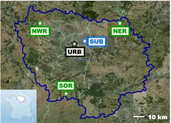
Six sampling sites were implemented, covering the region of Paris (see Fig. 1). These sites are part of the AIRPARIF Air Quality monitoring network, and are regarded as be-ing representative of background conditions (Ghersi et al., 2010). They were categorised according to criteria proposed by the European Environment Agency (Larssen et al., 1999). The first site is an urban (URB) station located in the city
centre of Paris (4th district, 48◦5005600N, 02◦2105500E, 20 m
above ground level, a.g.l.). The second site is a near-city or suburban (SUB) station located at 10 km northeast of
the URB station (48◦5205400N, 02◦3002300E, 5 m a.g.l.). The
third, fourth and fifth sites are rural stations located respec-tively at ca. 65 km northeast (NER), 50 km northwest (NWR)
and 60 km south (SOR) of the URB station (49◦0501500N,
03◦0403500E, 5 m a.g.l.; 49◦0304800N, 01◦5105900E, 5 m a.g.l.
and 48◦2104900N, 02◦1400700E, 5 m a.g.l., respectively). A
traffic (TR) station located at the ring road of Paris, at 9 km
west of the UR station was also implemented (48◦5100200N,
2◦1500900E, 5 m a.g.l.). This last station will not be described
here due to its specificity (traffic sources) whereas this paper aims at describing representative urban, suburban and rural backgrounds.
2.2 Aerosol sampling
Fine aerosol particles (PM2.5) were collected at each site
every day during 24 h (from 00:00 to 23:59 LT) during one year (from 11 September 2009 to 10 September 2010). Fil-ter sampling was performed using two collocated Leckel low volume samplers (SEQ47/50) at each station running at
2.3 m3h−1. One Leckel sampler was equipped with quartz
filters (QMA, Whatman, 47 mm diameter) for carbon analy-ses, the second with Teflon filters (PTFE, Pall, 47 mm diam-eter, 2.0 µm porosity) for gravimetric and ion measurements.
Before being sampled, QMA filters were baked at 480◦C
35 2
3
4 5
Fig. 1. Spatial distribution of the sampling sites in the region of Paris (Ile-de-France region). Source: 6
Google Earth. 7
Legend: SUB: SUBurban, URB: URBan, NER: North-East Rural, NWR: North-West Rural, SOR: SOuth 8
Rural. 9 10
11
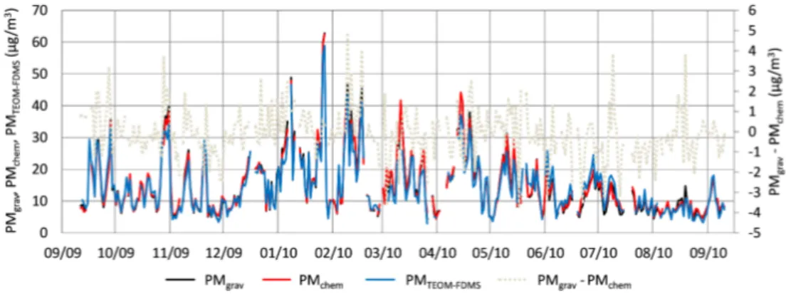
Fig. 2. Comparison between gravimetric (PMgrav), chemically reconstructed (PMchem) and TEOM-FDMS 12
(PMTEOM-FDMS) daily mass concentrations (µg/m3) at the urban site from 11 September 2009 to 10 13
September 2010. 14
Note: TEOM-FDMS measurements are conducted at 30°C and do not take into account semi-volatile 15 materials. 16 10 km NER NWR SOR URB SUB 0 10 20 30 40 50 60 70 09/09 10/09 11/09 12/09 01/10 02/10 03/10 04/10 05/10 06/10 07/10 08/10 09/10 Conc en tr atio ns (µ g /m 3)
PMgravPMgrav PMchemPMchem PMteom-fdmsPMTEOM-FDMS
Fig. 1. Spatial distribution of the sampling sites in the region of Paris (Ile-de-France region). Source: Google Earth. Legend: SUB: SUBurban, URB: URBan, NER: East Rural, NWR: North-West Rural, SOR: SOuth Rural.
for 48 h and PTFE filters pre-weighed as reported in Sciare et al. (2003). Field blanks were taken every two weeks for PTFE filters, and every week for QMA filters. A total of 4040 filters have been collected including 2085 QMA and 1955 PTFE filters. Few samples have been discarded because of power failures, chemical analysis problems, etc. (Table S1) and represent ca. 5 % of QMA and 5 % of PTFE filters. Once
sampled, filters were stored at −20◦C in a freezer prior to
chemical analyses.
2.3 Chemical analyses 2.3.1 Gravimetry
In order to minimise the influence of water adsorption, loaded and unloaded PTFE filters were equilibrated for 48 h at ambient temperature and below 30 % relative humidity (RH) prior to being weighed (MacMurry, 2000; Sciare et al., 2005). PTFE filters were then weighed with a microbalance (Sartorius, MC21S) with 1 µg sensitivity. Filter weighing was repeated until having a difference between two weighs be-low 5 µg. The overall error is estimated to be 10 µg which represents 3 ± 2 % of loaded filters (n = 1723; all sites, one-year measurements, blank filters excluded). Aerosol masses
(PMgrav)were deduced from the gravimetric measurements
done before and after sampling. Field blanks taken on the
field show an averaged PMgravof 7 ± 11 µg (n = 130), which
represents 2 ± 1 % of loaded filters (n = 1723), thus being below the overall microbalance error.
2.3.2 Ions
The following water-soluble major ions were analysed by Ion Chromatographs (IC): chloride, nitrate, sulfate, sodium, am-monium, potassium, magnesium and calcium. The analytical
protocol followed is thoroughly described by Sciare et al. (2008) and Guinot et al. (2007). Briefly, filter samples were extracted in 15 mL of Milli-Q water during 45 min in a sonic bath. To prevent bacteria activity, 50 µL of chloro-form was added. Samples were then filtered using Acrodisc filters (Pall Gelman) with a porosity of 0.4 µm. Cations were analysed on a 2 mm diameter CS12 pre-column and col-umn with an IC (Dionex, Model DX-600, USA), anions on a 2 mm diameter AS11 pre-column and column with an IC (Dionex, Model DX-600, USA). Both IC apparatus were equipped with a regent free system (automated eluent genera-tion and self-regenerating suppression). Semi-annual labora-tory IC inter-comparison studies were performed (accessible at http://qasac-americas.org/lis/summary/44) and showed er-rors of less than 5 % for every cited ion. Field blank measure-ment medians (n = 130) are 26, 29, 4, 9, 9, 4, 2 and 22 ppb
for Cl−, NO− 3, SO 2− 4 , Na +, NH+ 4, K +, Mg2+, and Ca2+,
re-spectively, which represent 16, 2, 0, 5, 1, 3, 6 and 24 % of the medians of loaded filters (n = 1723), respectively. Blank corrections have only been performed for chloride and cal-cium ions by subtracting blank medians to the loaded filter values.
2.3.3 Carbon
Elemental carbon (EC) and organic carbon (OC) were deter-mined by a thermal-optical method using a Sunset Labora-tory Carbonaceous Analyser (Sunset Lab., OR, USA) and the EUSAAR 2 protocol (transmission method) defined by Cav-alli et al. (2010). A detailed description concerning thermal-optical methods and the relevance of the protocol chosen can be found elsewhere (Chow et al., 1993; Schmid et al., 2001; Cavalli et al., 2010). The detection limit and the uncertainty given by the Sunset Company are estimated to be 0.2 µgC and 5 %, respectively, for EC and OC measurements. EC was not
detected in field blanks (0.0 ± 0.1 µgC cm−2, n = 252), and
OC was found with an average value of 1.1 ± 0.5 µgC cm−2
(n = 252). On average, this field blank value represents 15 ± 7 % of sampled filter’s OC concentrations (n = 1723). Blank corrections have been performed for OC concentra-tions by subtracting the blank average to the sampled filter values.
2.4 Chemical mass closure
Aerosol Chemical Mass Closure (CMC) consists in
compar-ing the sum of the major aerosol chemical species (PMchem)
with gravimetric measurements (PMgrav). When achieved
(i.e. when PMchem=PMgrav), CMC attests the consistency
of chemical analyses, and confirms that all the major aerosol
chemical species are taken into account. PMchemcalculation
is here expressed as:
[PMchem] = [Sea Salt] + [Dust] + [Secondary Inorganic (1)
Aerosols] + [Carbonaceous Matter]
Sea salt (ss-) concentrations are calculated from the six ma-jor ions accounting for more than 99 % of the mass of salts dissolved in seawater:
[Sea salt] = [Na+] + [Cl−] + [Mg2+] (2)
+[ss − K+] + [ss − Ca2+] + [ss − SO2−4 ]
with [ss-K+]= 0.036·[Na+]; [ss-Ca2+]= 0.038·[Na+] and
[ss-SO2−4 ]= 0.252·[Na+]
Typical seawater ion ratios based on the average seawater composition are taken from Seinfeld and Pandis (1998).
Different methods are used to calculate the mineral dust
fraction in PM2.5, and are based on its average elemental
composition from specific sites, or on specific tracers (Pet-tijohn, 1975; Malm et al., 1994; Guieu et al., 2002). Re-cently, nss-calcium has been used to estimate mineral dust in aerosols because of its abundance (Putaud et al., 2004a; Sciare et al., 2005). We used the 15 % contribution of nss-calcium in mineral dust determined by Guinot et al. (2007) in Paris:
[Dust] = [nss − Ca2+]/0.15 (3)
This is in agreement with the ratio of 18 % reported by Putaud et al. (2004b) in Monte Cimone (Italy) during non-Saharan dust periods. The resulting proportion of dust in
PM2.5 during the whole campaign ranges from 2 to 5 % on
average at the five sites (see Sect. 4.2.2). By changing this
ratio by ±3 %, the resulting proportion of dust in PM2.5
re-mains very low at the five sites (3 to 6 % and 2 to 4 % of
PM2.5with nss-Ca2+to dust ratios of 12 and 18 %,
respec-tively). In the frame of chemical mass closure, further in-vestigation allowing the estimation of dust will thus not be conducted.
Secondary inorganic aerosols (SIA) are calculated as:
[Secondary Inorganic Aerosols] = [nss − SO2−4 ] (4)
+[NO−3] + [NH+4]
where [nss-SO2−4 ] = [SO2−4 ] − [ss-SO2−4 ], “nss-” standing
for “non-sea-salt”.
Finally, carbonaceous matter can be expressed as:
[Carbonaceous Matter] = [EC] + [OM] (5)
with [OM] = fOC−OM·[OC].
The estimation of organic matter and more specifically of
2.5 Organic carbon to organic matter conversion factor
Organic matter (OM) is here inferred from filter OC measure-ments determined by the Sunset Laboratory analyser. The estimation of OM is of high complexity due to its varied chemical composition which changes according to location, season and time of the day (Turpin et al., 2000; Andrews et al., 2000). Turpin and Lim (2001) recommend the measure-ment of the average molecular weight per carbon weight in the location of interest; such measurements were not con-ducted in this study. In that case, they suggest the use of
an OC to OM conversion factor (fOC−OM)of 1.6 ± 0.2 for
urban aerosols and 2.1 ± 0.2 for nonurban aerosols. These factors were widely used in recent peer reviewed publica-tions (Terzi et al., 2010; Cheung et al., 2011; Rengarajan et al., 2011) despite their spatial and temporal dependencies.
We decided to estimate fOC−OM from our dataset by using
a method adapted from Guinot et al. (2007) who used the
chemical mass closure technique as a tool to assess fOC−OM
from OC measurements.
To infer fOC−OM, we assumed that CMC is achieved
(PMgrav=PMchem), and used Eq. (1) to write the following
equation:
fOC−OM=1/[OC] · ([PMgrav] −([Sea Salt] + [Dust] (6)
+[SIA] + [EC]))
This will allow us to find the “best guess” fOC−OM value
from our dataset. To simplify Eq. (6), a chemical fraction named “Remaining mass” (RM) has been defined in Eq. (7):
[Remaining Mass] = [PMgrav] −([SeaSalt] + [Dust] (7a)
+[SIA] + [EC])
thus leading to:
[Remaining Mass] = fOC−OM· [OC] (7b)
Two different methods were then used to estimate fOC−OM.
In the first method, RM concentrations are plotted against
OC concentrations and fOC−OMis the slope of the linear
re-gression (Eq. 7). We decided to use a linear function without y-intercept because of the analytical form of this equation. In
the second method, we numerically calculated fOC−OM
day-by-day from Eq. (6). Days with fOC−OMhigher than 3 and
lower than 1 were considered as physically meaningless and were therefore excluded from the dataset. These days repre-sent 6 to 14 % of the samples according to sites. Results will be discussed in Sect. 3.5.
2.6 Additional measurements
Meteorological parameters such as temperature, pressure, precipitation, wind speed and wind direction were pro-vided by the French national meteorological service “Meteo-France” from measurements recorded at Montsouris (14th
district, 48◦4902000N, 02◦2001800E) located at about 5 km
south of the URB station. Boundary Layer Height (BHL) is taken from simulations with the PSU/NCAR mesoscale model (MM5; Dudhia, 1993; Grell et al., 1994). In the vertical, 23 sigma layers extend up to 100 hPa. MM5 is forced by the final analyses from the Global Forecast Sys-tem (GFS/FNL) operated daily by the American National Centers for Environmental Prediction (NCEP), using the grid nudging (grid FDDA) option implemented within MM5. The Medium Range Forecast scheme (MRFPBL) has been used to parameterize turbulence in the boundary layer (Tro¨en and Mahrt, 1986). Air mass back trajectories were calculated us-ing the Hybrid Sus-ingle Particle Lagrangian Integrated Trajec-tory (HYSPLIT) model (Draxler and Rolph, 2011).
3 Results
3.1 Representativeness of the campaign
The meteorological conditions and the PM level representa-tiveness of the studied period were investigated and reported in Fig. S1. Air temperatures measured during our campaign were comparable to standard values determined by Meteo-France (calculated following Arguez and Vose, 2011), show-ing however lower values durshow-ing winter (DJF, Fig. S1a). Levels of precipitation showed discrepancies in comparison with standard values (Fig. S1b). More specifically, Septem-ber 2009 and April 2010 were particularly dry, unusual snow events occurred during January 2010 and heavy rains during July and August 2010. Paris is typically characterised by a dominance of south to southwest winds (ca. 35 %) and to a lesser extent north to northeast winds (ca. 20 %) (Fig. S1c). The studied period showed similar trends although a stronger contribution of the northeast sector was observed.
Finally, our yearly average PM2.5 mass concentration of
18.4 µg m−3was characteristic of a usual year (R&P Tapered
Element Oscillating Microbalance – Filter Dynamic Mea-surement System, TEOM-FDMS, (Rupprecht and Patashnik Co., Inc.; Patashnik and Rupprecht, 1991) data corrected for semi-volatile materials at the urban site). It was lower than in 2007 (ca. −11 %), but higher than in 2008 (ca. +16 %, values calculated from TEOM-FDMS data measured at a similar ur-ban site of the Airparif network).
3.2 Chemical composition of PM2.5
Table 1 reports statistics on the chemical composition of
PM2.5at the five sites, on the whole sample set. PM2.5levels
range from 10.8 to 15.2 µg m−3on average according to sites.
Fine aerosols are primarily made of OC (2.1–3.2 µg m−3),
ni-trate (2.2–2.9 µg m−3), sulfate (1.8–2.1 µg m−3)and
ammo-nium (1.2–1.5 µg m−3); and to a lesser extent of EC (0.4–
1.4 µg m−3) and minor ions (less than 0.2 µg m−3 for Cl−,
Na+, K+, Ca2+and Mg2+). Further discussion will be
T able 1. Chemical composition (µg m − 3 ) of PM 2 .5 at the fi v e sites during the one-year period . SUB URB AN URB AN NOR TH EAST R URAL NOR TH WEST R URAL SOUTH R URAL n = 348 n = 335 n = 330 n = 359 n = 351 min ma x med av std min max med av std min max med av std min max med av std min max med av std Mass 3.7 62.6 11.9 15.2 10.5 3.9 62.8 11.6 14.8 9.6 2.8 48.6 9.6 12.6 8.6 2.1 61.4 8.7 11.7 9.5 0.7 49.4 7.9 10.8 8.4 OC 0.5 19.8 2.5 3.2 2.5 0.6 12.7 2.6 3.0 1.7 0.4 13.1 2.2 2.9 2.2 0.2 12.8 1.6 2.2 1.9 0.3 10.6 1.7 2.1 1.5 NO − 3 < LOQ 17. 5 1.1 2.9 3.6 < LOQ 1 7.1 1.1 2.9 3.7 < LOQ 16.6 0.9 2.2 2.9 < LOQ 18.3 0.9 2.6 3.5 0.0 18.2 0.8 2.2 3.1 SO 2 − 4 0.2 10.1 1.7 2.1 1.7 0.2 11.2 1.6 2.0 1.6 0.2 9.6 1.5 1.9 1.4 0.2 10.9 1.5 1.9 1.6 0.1 9.6 1.4 1.8 1.6 NH + 4 0.1 8.1 0.8 1.5 1.6 0.0 9.0 0.7 1.4 1.6 0.1 7.2 0.7 1.2 1.3 < LOQ 8. 0 0.7 1.3 1.5 0.1 7.9 0.7 1.2 1.4 EC 0.3 5.3 1.2 1.3 0.7 0.1 4.5 1.3 1.4 0.7 0.1 1.6 0.5 0.5 0.3 0.1 2.3 0.4 0.5 0.3 0.0 1.8 0.4 0.4 0.3 Cl − < LOQ 1.6 5 0.11 0.18 0.21 < LOQ 1 .88 0.11 0.19 0.23 < LOQ 1.73 0.08 0.16 0.21 < LOQ 1.42 0.09 0.18 0.22 < LOQ 1 .72 0.07 0.14 0.19 Na + < LOQ 1.0 8 0.11 0.16 0.15 < LOQ 1 .19 0.11 0.18 0.17 < LOQ 1.22 0.09 0.14 0.14 < LOQ 0.9 4 0.11 0.16 0.15 < LOQ 1 .01 0.08 0.13 0.13 K + < LOQ 0.7 4 0.08 0.13 0.12 < LOQ 0 .73 0.07 0.12 0.12 < LOQ 1.59 0.07 0.12 0.13 < LOQ 0.7 2 0.06 0.11 0.12 < LOQ 0 .61 0.06 0.10 0.10 Ca 2 + < LOQ 1.2 9 0.06 0.08 0.09 < LOQ 1 .09 0.09 0.12 0.12 < LOQ 0.34 0.04 0.05 0.04 < LOQ 0.3 1 0.05 0.06 0.05 < LOQ 0 .30 0.03 0.04 0.04 Mg 2 + < LOQ 0.1 8 0.02 0.03 0.02 < LOQ 0 .16 0.02 0.03 0.02 < LOQ 0.16 0.02 0.02 0.02 < LOQ 0.13 0.02 0.03 0.02 < LOQ 0 .15 0.01 0.02 0.02 Le gend: LOQ: Limit of Quantification.
3.3 Comparison between filter and on-line determined masses
We investigated the atmospheric consistency of our PM2.5
measurements, and attempted to estimate artefacts associated with filter sampling (Zhang and McMurry, 1987; Mc Dow and Huntzicker, 1990; Turpin et al., 2000). A conventional on-line automatic system (TEOM-FDMS) was running dur-ing the campaign at the urban station only and is used by Air-parif since 2007 (AirAir-parif, 2012). Gravimetric and TEOM-FDMS determined masses are compared in Figs. 2 and 3.
TEOM-FDMS was running at 30◦C and was not corrected
for semi-volatile materials (i.e. only the reference signal of the TEOM-FDMS was used here, without taking into ac-count the SVM mass provided by the FDMS), in order to be as close as possible to our laboratory conditions. Very similar temporal variations are observed in Fig. 2 for both datasets for the whole duration of the campaign. TEOM-FDMS data plotted against gravimetric mass concentrations
show a very good correlation (r2=0.94, n = 318, Fig. 3).
However, filter measurements exhibit mass concentrations about 6 % higher than the on-line method (slope ± 1 stan-dard error = 0.938 ± 0.007). This can be related to tempera-ture differences during filter sampling (ambient temperatempera-ture)
and TEOM-FDMS measurements (30◦C), leading in the
lat-ter case to a partial volatilization of semi-volatile malat-terials. Absorption of volatile organic compounds (VOC) (Turpin et al., 1994, 2000) and/or water onto filters (Quinn and Coff-man, 1998; Speer et al., 2003; Hueglin et al., 2005) could also enhance filter masses. In addition, taking into account semi-volatile materials in TEOM-FDMS measurements (i.e. adding the SVM mass provided by the FDMS to the refer-ence signal of the TEOM-FDMS) leads to higher concen-trations compared with the gravimetric method (18.4 versus
14.8 µg m−3, respectively, on average at the URB site). The
former method is regarded as an equivalent method to the EU reference method (EN 14907), whereas the latter does not fulfil EU requirements (by operating below 30 % RH in-stead of at 50 % RH). It should thus be borne in mind that
our gravimetric method will underestimate PM2.5mass
com-pared to EU reference methods by ca. 20 % on average.
3.4 Comparison between filters and on-line determined chemical components
The chemical results obtained at the urban site were com-pared with real-time chemical analysers that were set in the Paris urban area (ca. 2 km south of the URB site) as part of the wintertime intensive field experiment of the European programme MEGAPOLI (15 January–15 February 2010). Such comparison may provide insights into the importance of positive and negative artefacts associated with our unde-nuded filter sampling of semi-volatile species (typically am-monium nitrate and organic aerosols).
Fig. 2. Gravimetric (PMgrav), chemically reconstructed (PMchem), TEOM-FDMS (PMTEOM-FDMS)and gravimetric minus chemically
re-constructed (PMgrav−PMchem)daily mass concentrations (µg m−3)at the urban site from 11 September 2009 to 10 September 2010. Note:
TEOM-FDMS measurements are conducted at 30◦C and do not take into account semi-volatile materials.
Fig. 3. Comparison between gravimetric (PMgrav) and
TEOM-FDMS (PMTEOM-FDMS)daily mass concentrations (µg m−3)at the urban site from 11 September 2009 to 10 September 2010 (n = 318). Error bars represent uncertainties associated with PMgrav
and PMTEOM-FDMSmeasurements. Note: TEOM-FDMS
measure-ments are conducted at 30◦C and do not take into account semi-volatile materials. The slope is given ±1 standard error.
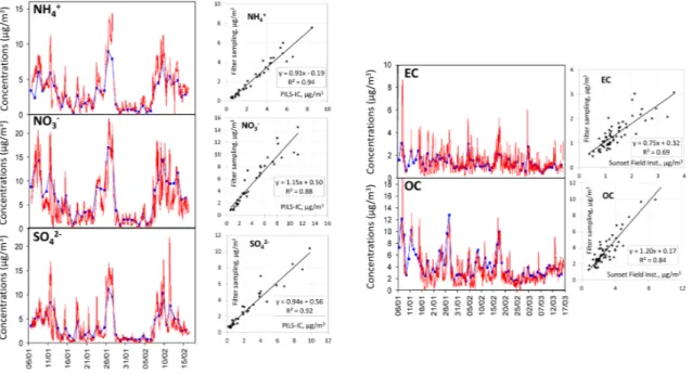
Concerning ion concentrations, filter measurements were compared for a period of 40 days (6 January–15 February 2010) with a Particle-Into-Liquid-Sampler (PILS; Orsini et al., 2003) coupled with two IC results. The PILS-IC
in-strument measures selected anions and cations (Cl−, NO−
3,
SO2−4 , Na+, NH+4, K+, Mg2+, Ca2+)every 10 min in PM2.5.
Settings used here for the PILS-IC measurements are similar to those reported in Sciare et al. (2011) and will be presented elsewhere (Crippa et al., 2013). The liquid-based aerosol col-lection principle used in the PILS-IC avoids the positive and negative filter sampling artefacts usually associated with the
collection of semi-volatile ammonium nitrate in PM2.5.
Un-certainties of the PILS-IC measurements are typically within 20 % (Weber et al., 2003; Orsini et al., 2003; Hogrefe et al., 2004; Takegawa et al., 2005). They are compared with the filter sampling results in Fig. 4a for the three major ions
(NH+4; NO−3, SO2−4 ). Very satisfactory results are obtained
(r2ranging from 0.88 to 0.94) with slopes close to 1
(rang-ing from 0.91 to 1.15) and y-intercepts close to zero (rang(rang-ing
from −0.19 to +0.56 µg m−3), i.e. in the range of
uncertain-ties given by the two techniques. One of the most important points is the absence of significant discrepancies concerning nitrate, which is a semi-volatile species exhibiting high con-centrations during winter in Paris (Favez et al., 2007). Note
that the comparison results obtained for the other ions (Cl−,
Na+, Mg2+)are also very satisfactory (r2ranging from 0.85
to 0.90) with slopes close to 1 (ranging from 1.11 to 1.19). Filter sampling EC and OC concentrations were com-pared for a period of 70 days (6 January–15 March 2010) with semi-continuous hourly measurements of VOC denuded
EC and OC concentrations in PM2.5, obtained using an
OCEC Sunset field instrument (Sunset Laboratory, Forest Grove, OR, USA; Bae et al., 2004). The default thermal programme (National Institute for Occupational Safety and Health, NIOSH; Birch and Cary, 1996) was used in this instrument. Measurement uncertainty given by the OCEC Sunset field instrument is poorly described in the literature and an estimate of 20 % was considered following Peltier et al. (2007). Comparisons between filter sampling and semi-continuous EC and OC measurements are performed in
Fig. 4b and show a relatively good agreement (r2 of 0.69
and 0.84) with slopes of 0.75 and 1.20, and y-intercepts of
+0.32 and +0.17 µg m−3for EC and OC, respectively. Slope
differences may partly originate from the different thermal
programs used, having a nearly 200◦C difference for the last
temperature plateau under Helium (Cavalli et al., 2010). In order to test this assumption, a comparison was performed for Total Carbon (TC) measurements and showed a very
Fig. 4. Comparison between filter and on-line measurements for a 40-day period for the major ions (Fig. 4a), and for a 70 day period for carbonaceous matter (Fig. 4b).
good correlation (r2=0.87) with a slope close to one (1.09)
and a y-intercept close to zero (+0.4 µg m−3).
3.5 OC to OM conversion factor
Results concerning the OC to OM conversion factor are re-ported in Table 2. Concerning the first method (linear regres-sion), very good correlations between RM and OC concen-trations were observed for the whole duration of the project,
at every site (r2higher than 0.90, Fig. S2). This suggests that
the unidentified chemical fraction RM is directly related to OC. In other terms, this confirms that all the major chemical components are taken into account in Eq. (1), and that the de-fined “Remaining Mass” fraction can be regarded as organic matter like. It should be noted that no significant amount of water is adsorbed onto filters because weighing is performed under dry conditions (RH below 30 %, Sect. 2.3.1). Conver-sion factors are slightly lower for the urban and suburban sta-tions than for the rural ones (1.95, 1.98, 2.03, 2.08 and 2.12 for SUB, URB, NER, NWR and SOR, respectively). Organic matter is generally more oxidised in rural areas, leading to higher conversion factors (Turpin and Lim, 2001). The small discrepancy observed between the different types of environ-ments in the region of Paris may be explained by the homo-geneity of organic carbon concentrations, suggesting the im-portance of imported sources (see Sect. 4.2). Seasonal
vari-ations of fOC−OM are illustrated in Fig. S3. This factor is
relatively stable all along the year at the five sites, ranging between 1.8 and 2.2; different patterns are observed from one season to another according to sites, thus suggesting the ab-sence of clear seasonal variations.
Very similar conclusions can be drawn concerning the sec-ond method (day-by-day calculation), which leads to slightly lower (p<0.005 using the Welch’s t test; Welch, 1947) con-version factors at SUB and URB than at the rural sites (1.96, 1.92, 2.08, 2.05 and 2.09 for SUB, URB, NER, NWR and SOR, respectively). High relative standard deviations are ob-served at every site, ranging from 15 to 20 %. This suggests that the organic matter chemical composition is strongly daily dependant, which can be related to the daily changing meteorological conditions (as air mass origins and air tem-peratures; see Sect. 4.1). No clear seasonal pattern (Fig. S3) is observed with this second method as well. Comparable
fOC−OM values are found with both methods in every
en-vironment, showing relative differences below 3 % for each site. The first method is however preferred as no days are excluded from the dataset and because of its more advanced mathematical approach.
We chose to apply an OC to OM conversion factor equal to 1.95 for the suburban and urban sites, and of 2.05 for the three rural sites, for the whole duration of the project. By choosing these factors, we wanted to give an insight of the general chemical properties of OM in the region, and to allow its comparison between sites. The chosen conver-sion factors set among the values suggested by Turpin and Lim (2001) of 1.6 ± 0.2 for urban areas and 2.1 ± 0.2 for non-urban areas, and Kiss et al. (2002) of 1.9–2.0 in a ru-ral area. It is higher than the factors used in previous stud-ies in the region of Paris by Guinot et al. (2007) of 1.8 and Favez et al. (2009) of 1.7 (this last factor was recalculated from water-soluble organic carbon and water-insoluble or-ganic carbon contents), which can be related to differences
Table 2. Determination of the OC to OM conversion factor (fOC−OM)at the five sites, from 11 September 2009 to 10 September 2010, using two analytical methods.
SUBURBAN URBAN NORTH EAST RURAL NORTH WEST RURAL SOUTH RURAL
Methods 1 2 1 2 1 2 1 2 1 2
n 348 326 335 307 330 297 359 309 351 306
fOC−OM 1.95 ± 0.02 1.96 ± 0.33 1.98 ± 0.02 1.92 ± 0.33 2.03 ± 0.02 2.08 ± 0.34 2.08 ± 0.02 2.05 ± 0.38 2.12 ± 0.02 2.09 ± 0.38
r2 0.94 – 0.90 – 0.94 – 0.92 – 0.90 –
Legend: Method 1: linear regression “y = a · x” from Eq. (7). fOC−OMis the slope of the linear regression. Standard deviation is calculated from the standard error of the slope. Method 2: day-by-day calculation from Eq. (6). Days with fOC−OMhigher than 3 and lower than 1 were excluded. fOC−OMis the arithmetic mean.
n: number of samples.
in OC/EC separation methods (e.g. differences in thermo-optical protocols). It should also be mentioned that the rel-atively high conversion factors found in our study could be related to (i) possible aerosol water content – even at RH be-low 30 %, which is not taken into account in our mass closure calculation and (ii) possible errors from the applied functions defined for the calculation of sea salt and dust (see Putaud et al., 2010 for a quantification of these errors).
Gravimetric, chemically reconstructed and on-line
deter-mined PM2.5 mass concentrations are compared in Fig. 2.
Very good correlations are found between the three datasets,
with r2 of 0.98 and 0.94, and slopes of 1.00 and 1.05 for
chemically reconstructed against gravimetric, and against TEOM-FDMS determined mass concentrations, respec-tively. This confirms the consistency of our measurements and the conversion factors chosen to estimate organic matter.
4 Discussion
Section 4.1 will describe the temporal variability of PM2.5
mass and major chemical constituents, whereas Sect. 4.2 will focus on their spatial variability.
4.1 Temporal variability of PM2.5
4.1.1 Daily temporal variability of fine aerosols
Daily temporal variability of fine aerosol chemical compo-sition at the suburban site is reported in Fig. 5. Similar pat-terns are observed at the five stations (Fig. S4 and Sect. 4.2) making the conclusions drawn for this site relevant for the four others. Strong variability can be observed from one day to another, for PM mass and chemical composition.
On the whole duration of the project PMgrav is on average
15.2 ± 10.5 µg m−3, and ranges from 3.7 to 62.6 µg m−3
(Ta-ble 1; unless otherwise stated all the figures mentioned in this Sect. 4.1 refer to the SUB site). Most pollution events occur during late autumn, winter and early spring (from De-cember to April) and are associated with marked increases of secondary inorganic species (e.g. on 26 January 2010:
PMgravand SIA concentrations are 58.7 and 32.1 µg m−3,
re-spectively). Organic matter also significantly contributes to the enhancement of PM mass during pollution events (e.g.
more than 60 % of PMgravon 7 January 2010, with [PMgrav]
= 62.6 µg m−3), contrarily to sea salt, dust and EC. The
strong daily variability of PM concentration and composi-tion can be explained by the variacomposi-tions of source emission in-tensities, atmospheric processes (e.g. Healy et al., 2012) and meteorological parameters (e.g. Galindo et al., 2011; Mar-tin et al., 2011; Georgoulias and Kourtidis, 2011). A focus will be made on the latter variable and especially on tem-perature, boundary layer height (BLH), precipitation and air mass origins. Although those meteorological parameters can be highly correlated, their individual influence will be high-lighted during specific polluted and clean conditions.
4.1.2 Influence of meteorological parameters
Temperature modifies the emission of secondary PM pre-cursors such as biogenic VOCs during summer (Fowler et al., 2009, and references therein), the formation of temper-ature inversion during winter (Stull, 1988) or the condensa-tion of high saturacondensa-tion vapour pressure compounds such as nitric acid (Monks et al., 2009; Hueglin et al., 2005). In the
city of Paris, low temperatures (daily average below 0◦C)
often lead to high pollution events ([PMgrav] > 40 µg m−3)
mainly due to the increased contribution of SIA (Fig. 6).
During winter (DJF) SIA concentrations exceed 10 µg m−3
during 35 days, contributing 50 ± 9 % of PMgravunder
tem-peratures of −0.7 ± 2.9◦C on average. SIA are thus a
ma-jor cause of the high PM2.5 concentrations observed in the
region of Paris during cold events, hence asking for partic-ular attention for the implementation of efficient abatement strategies. Whereas nitrate concentrations are enhanced dur-ing cold periods because of thermodynamic processes (Clegg et al., 1998), high nss-sulfate concentrations are certainly due to mid- or long-range transport episodes that are related to anticyclonic conditions, eastern air masses and low temper-atures (see below and Sect. 4.2). (In the following, mid- or long-range transport will refer to transport from outside the region of Paris, the exact origin not being quantitatively as-sessed at the current state of analysis.) In fact, nss-sulfate is mostly produced from cloud processing over large scales
rather than from local gas phase oxidation of SO2 (Putaud
et al., 2004a). Finally, nitrate and nss-sulfate are fully
37 1
Fig. 5. Daily variation of fine aerosol chemical composition at the suburban site from 11 September 2
2009 to 10 September 2010. 3
4
Fig. 6. Comparison between daily nitrate, nss-sulfate and ammonium concentrations (µg/m3) and 5
temperatures (°C) at the suburban site from 11 September 2009 to 10 September 2010. 6
7
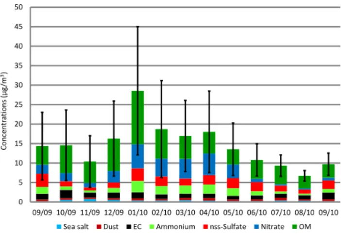
Fig. 7. Monthly mean concentrations (µg/m3) of fine aerosol chemical composition at the suburban 8
site from 11 September 2009 to 10 September 2010. Error bars represent the standard deviation 9
(±1σ) of fine aerosol mass concentrations. 10 11 0 10 20 30 40 50 60 70 09/09 10/09 11/09 12/09 01/10 02/10 03/10 04/10 05/10 06/10 07/10 08/10 09/10 C onc en tr ations (µg /m 3)
Sea Salt Dust EC Ammonium nss-Sulfate Nitrate OM
-10 -5 0 5 10 15 20 25 30 0 2 4 6 8 10 12 14 16 18 20 09/09 10/09 11/09 12/09 01/10 02/10 03/10 04/10 05/10 06/10 07/10 08/10 09/10 Tem p er atu re (° C) C onc en tr ations (µg /m 3)
Nitrate nss-Sulfate Ammonium Temperature
0 5 10 15 20 25 30 35 40 45 50 09/09 10/09 11/09 12/09 01/10 02/10 03/10 04/10 05/10 06/10 07/10 08/10 09/10 C onc en tr ations (µg /m 3)
Sea salt Dust EC Ammonium nss-Sulfate Nitrate OM
Fig. 5. Daily variation of fine aerosol chemical composition at the suburban site from 11 September 2009 to 10 September 2010.
37 1
Fig. 5. Daily variation of fine aerosol chemical composition at the suburban site from 11 September 2
2009 to 10 September 2010. 3
4
Fig. 6. Comparison between daily nitrate, nss-sulfate and ammonium concentrations (µg/m3) and 5
temperatures (°C) at the suburban site from 11 September 2009 to 10 September 2010. 6
7
Fig. 7. Monthly mean concentrations (µg/m3) of fine aerosol chemical composition at the suburban 8
site from 11 September 2009 to 10 September 2010. Error bars represent the standard deviation 9
(±1σ) of fine aerosol mass concentrations. 10 11 0 10 20 30 40 50 60 70 09/09 10/09 11/09 12/09 01/10 02/10 03/10 04/10 05/10 06/10 07/10 08/10 09/10 C onc en tr ations (µg /m 3)
Sea Salt Dust EC Ammonium nss-Sulfate Nitrate OM
-10 -5 0 5 10 15 20 25 30 0 2 4 6 8 10 12 14 16 18 20 09/09 10/09 11/09 12/09 01/10 02/10 03/10 04/10 05/10 06/10 07/10 08/10 09/10 Tem p er atu re (° C) C onc en tr ations (µg /m 3)
Nitrate nss-Sulfate Ammonium Temperature
0 5 10 15 20 25 30 35 40 45 50 09/09 10/09 11/09 12/09 01/10 02/10 03/10 04/10 05/10 06/10 07/10 08/10 09/10 C onc en tr ations (µg /m 3)
Sea salt Dust EC Ammonium nss-Sulfate Nitrate OM
Fig. 6. Comparison between daily nitrate, nss-sulfate and ammonium concentrations (µg m−3)and temperatures (◦C) at the suburban site from 11 September 2009 to 10 September 2010.
mol m−3: slope = 0.96; r2=0.96, n = 348), which
there-fore follows the same pattern. Similar correlations between high atmospheric concentrations and low temperatures are also found for organic matter, which can be explained by strong biomass burning sources – related to domestic heat-ing – in the region of Paris (Favez et al., 2009; Sciare et al., 2011; Healy et al., 2012) and probably to the condensation of semi-volatile organic species as observed in many European areas (Putaud et al., 2004a).
However, days exhibiting high SIA and PM concentrations cannot solely be explained by low temperatures (e.g. 14 April 2010, 10 May 2010, etc.), meteorological parameters such as precipitation and boundary layer height should be regarded as well (Fig. S5). BLH plays an important role in determin-ing the transport, storage and dispersion of atmospheric pol-lutants (Salmond and McKendry, 2005) and is responsible for high PM daily variability in Paris during all the campaign. As an illustration, during two following days (31 October 2009
and 1 November 2009), PM2.5 concentrations were reduced
by a factor of 3.5 (37.7 and 10.6 µg m−3, respectively) mainly
due to the increase by a factor of 2.8 of the BLH (288 and 820 m, respectively). In addition, the wet removal by precip-itation is known to be the most efficient atmospheric aerosol sink (Radke et al., 1980) and contribute to low concentration
days (< 10 µg m−3)in Paris, especially from November to
April because of heavy rains (typically higher than 5 mm per day).
Finally, air mass origins can be a strong cause of PM daily variability because of the flat topography of the region, and the contrasted surrounding environments (marine versus con-tinental areas). This is illustrated in Fig. S5 where two-days back trajectories were calculated every four hours for two typical types of air masses in the region, using HYSPLIT (Draxler and Rolph, 2011). Air masses originating from con-tinental Europe (northeast to east of France) lead to high PM loadings and high contents of SIA, especially during win-ter, whereas air masses coming from marine sectors (west and north of France) bring much lower aerosol content. In fact, one of the highest PM pollution peaks of the campaign
(26 January 2010, [PMgrav] = 58.7 µg m−3)is mainly due to
mid- or long-range transport from continental Europe
(con-centrations ranging from 47.2 to 61.4 µg m−3 at the other
sites) and is predominantly made of SIA (50 % of [PMgrav]).
(Mid- or long-range transport from continental Europe will be named continental transport or continental import later on.) Contrarily, under marine air masses that are poorly
influ-enced by anthropogenic pollution, PM2.5 concentrations are
typically below 10 µg m−3 (e.g. 6.5 and 8.6 µg m−3 for 13
September 2009 and 25 October 2009, respectively). These conclusions, regarding the significant contribution of east-ern mid- or long-range pollution in the region of Paris, are
M. Bressi et al.: A one-year comprehensive chemical characterisation of fine aerosol 7835
in agreement with what Bessagnet et al. (2005), Sciare et al. (2010, 2011) and Healy et al. (2012) reported in short-term studies in this city in winter and spring. We attempted to quantify this phenomenon by focusing on days showing
PMgrav concentrations higher than 25 µg m−3, which is the
PM2.5 2015 EU annual limit value and the PM2.524 h-mean
World Health Organization Air Quality Guideline value. A total of 50 days fulfilled the aforementioned criterion on the whole duration of the campaign. Three categories were de-fined: days with air masses originating from the northeast to the east of France, days with BLH below 400 m (represent-ing the 10th percentile of BLH values) and days that do not fit either of both above mentioned criteria. We found that 66 % of the polluted days can be attributed to continental import (among which 12 % show low BLH), 20 % exhibit low BLH with other air mass origins, and 14 % cannot be explained by the previous factors. Therefore, in Paris, two third of the
days exceeding the 2015 EU annual PM2.5 limit value are
due to continental import from the northeast to the east of France, questioning the efficiency of local, regional and even national abatement strategies during pollution episodes, sug-gesting instead collaborative works with neighbouring coun-tries on these topics. It should be added that French emissions can also impact surrounding areas as reported in Bessagnet et al. (2005), being significantly influential on Great Britain, Belgium, Germany, the Netherlands and Eastern Europe.
4.1.3 Monthly and seasonal variability of PM2.5 Keeping in mind the high daily variability of PM mass and chemical composition, their monthly and seasonal trends have been studied (Figs. 7 and S6). On the annual scale, Paris
(URB and SUB sites) exhibits its highest PM2.5
concentra-tions during late autumn, winter and early spring (higher
than 15 µg m−3on average, from December to April),
inter-mediates during late spring and early autumn (between 10
and 15 µg m−3 during May, June, September, October and
November) and the lowest during summer (below 10 µg m−3
during July and August). This pattern is mainly driven by OM and SIA concentrations that are the main components of fine aerosol (Fig. 7). Figure S6 shows that OM monthly mean concentrations significantly increase from autumn to winter (e.g. 2.5 times higher from November to January), slightly decrease from winter to early spring (e.g. −28 % from February to April), and remain fairly constant until the
end of the campaign (4.0 ± 0.7 µg m−3from June to
Septem-ber). During autumn and winter this pattern can be explained by stronger emissions of wood burning sources (Favez et al., 2009; Sciare et al., 2011, Sect. 4.2.3), whereas during spring and summer OM concentrations are likely related to bio-genic emissions and secondary organic aerosol formations (Jacobson et al., 2000, and references therein). Nitrate con-centrations are, on the other hand, on average significantly higher during winter and early spring months (JFMAM) than
the rest of the year (4.6 ± 1.2 µg m−3and 1.1 ± 0.8 µg m−3,
37 1
Fig. 5. Daily variation of fine aerosol chemical composition at the suburban site from 11 September 2
2009 to 10 September 2010. 3
4
Fig. 6. Comparison between daily nitrate, nss-sulfate and ammonium concentrations (µg/m3) and 5
temperatures (°C) at the suburban site from 11 September 2009 to 10 September 2010. 6
7
Fig. 7. Monthly mean concentrations (µg/m3) of fine aerosol chemical composition at the suburban 8
site from 11 September 2009 to 10 September 2010. Error bars represent the standard deviation 9
(±1σ) of fine aerosol mass concentrations. 10 11 0 10 20 30 40 50 60 09/09 10/09 11/09 12/09 01/10 02/10 03/10 04/10 05/10 06/10 07/10 08/10 09/10 C onc en tr ations (µg /m 3)
Sea Salt Dust EC Ammonium nss-Sulfate Nitrate OM
-10 -5 0 5 10 15 20 25 30 0 2 4 6 8 10 12 14 16 18 20 09/09 10/09 11/09 12/09 01/10 02/10 03/10 04/10 05/10 06/10 07/10 08/10 09/10 Tem p er atu re (° C) C onc en tr ations (µg /m 3)
Nitrate nss-Sulfate Ammonium Temperature
0 5 10 15 20 25 30 35 40 45 50 09/09 10/09 11/09 12/09 01/10 02/10 03/10 04/10 05/10 06/10 07/10 08/10 09/10 C onc en tr ations (µg /m 3)
Sea salt Dust EC Ammonium nss-Sulfate Nitrate OM Fig. 7. Monthly mean concentrations (µg m−3) of fine aerosol chemical composition at the suburban site from 11 September 2009 to 10 September 2010. Error bars represent the standard deviation (±1σ ) of fine aerosol mass concentrations.
respectively), partly because of thermodynamic conditions favouring the partitioning of this molecule into the particu-late phase (Clegg et al., 1998). Non-sea-salt sulfate exhibits
lower concentrations (< 1.5 µg m−3)during autumn (OND)
and mid-summer (JA), because Paris is less exposed to con-tinental advection during these months (Airparif and LSCE, 2012). Ammonium follows seasonal variations halfway be-tween nss-sulfate and nitrate as it fully neutralizes both com-pounds. EC and mineral dust do not display any seasonal pattern with stable concentrations all along the year that are
1.3 ± 0.3 and 0.5 ± 0.1 µg m−3, respectively, on average and
calculated from monthly means. Finally sea salt monthly variations are clearly related to wind directions, and show slightly higher concentrations during autumn (OND) as air masses coming from marine regions were prevalent (Airparif and LSCE, 2012).
4.2 Spatial variability of PM2.5
4.2.1 PM2.5mass concentrations
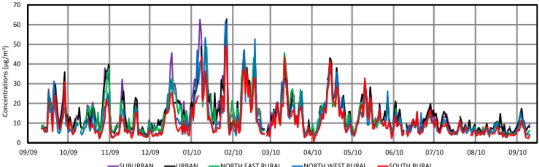
Spatial variability of fine aerosol in the region of Paris will first be discussed by comparing atmospheric mass concentra-tions determined gravimetrically at the five sites (Fig. 8). PM concentrations are surprisingly very similar at the regional scale, during most of the one-year project. Very good
correla-tions are found between urban and suburban sites (r2=0.94,
slope = 0.99, n = 335), good correlations are found between
rural sites (e.g. for NWR plotted against SOR sites, r2=
0.83, slope = 1.08, n = 351) and, more surprisingly, between urban and rural sites (e.g. for URB plotted against NER sites,
r2=0.84, slope = 1.06, n = 330). Interestingly, when
focus-ing on individual days a very high temporal variability is generally observed at the same time at the five sites. For
in-stance, PMgravlevels range from 49.4 to 62.0 µg m−3on 27
38 1
Fig. 8. Comparison between PM2.5 daily mass concentrations (gravimetric measurements) at the five 2
sites during the one-year period. 3
4
5
Fig. 9. Annual average chemical composition of PM2.5 (µg/m3; %) at the five sites from 11 September 6 2009 to 10 September 2010. 7 0 10 20 30 40 50 60 70 09/09 10/09 11/09 12/09 01/10 02/10 03/10 04/10 05/10 06/10 07/10 08/10 09/10 C onc en tr ations (µg /m 3)
SUBURBAN URBAN NORTH EAST RURAL NORTH WEST RURAL SOUTH RURAL
5.9; 47% 2.2; 17% 1.9; 15% 1.2; 10% 0.5; 4% 0.3; 2% 0.4; 3% 0.2; 2% NORTH EAST RURAL
OM Nitrate nss-Sulfate Ammonium EC Dust Sea salt Unaccounted mass
[PM2.5]=12.6 µg/m3 4.3; 40% 2.2; 21% 1.8; 16% 1.2; 11% 0.4; 4% 0.3; 3% 0.3; 3% 0.2; 2% SOUTH RURAL [PM2.5]=10.8 µg/m3 4.5; 38% 2.6; 22% 1.9; 16% 1.3; 12% 0.5; 4% 0.4; 3% 0.4; 4% 0.2; 1% NORTH WEST RURAL[PM2.5]=11.7 µg/m3
5.8; 39% 2.9; 20% 2.0; 13% 1.4; 10% 1.4; 10% 0.8; 5% 0.5; 3% 0.0; 0% URBAN [PM2.5]=14.8 µg/m3 6.3; 42% 2.9; 19% 2.0; 13% 1.5; 10% 1.3; 9% 0.5; 3% 0.4; 3% 0.2; 1% SUBURBAN [PM2.5]=15.2 µg/m3 5.9; 47% 2.2; 17% 1.9; 15% 1.2; 10% 0.5; 4% 0.3; 2% 0.4; 3% 0.2; 2% NORTH EAST RURAL [PM2.5]=12.6 µg/m3
Fig. 8. Comparison between PM2.5daily mass concentrations (gravimetric measurements) at the five sites during the one-year period.
according to sites; therefore after only 2 days, PM levels have been reduced by a factor ranging from 10 to 14 according to sites. This suggests that, in the region of Paris, background
PM2.5levels are mainly controlled by regional instead of
lo-cal slo-cale phenomena, which is in agreement with the above mentioned influences of mesoscale meteorological parame-ters and mid- or long-range transport (Sect. 4.1; Sciare et al., 2010).
Discrepancies between the different sites can however be noticed, with decreased concentrations when shifting from urban and suburban to rural sites, which is in agreement with most European environments (Querol et al., 2004; Van Dingenen et al., 2004; Putaud et al., 2004a). In fact,
an-nual PMgrav mean concentrations are 15.2, 14.8, 12.6, 11.7
and 10.8 µg m−3 for SUB, URB, NER, NWR and SOR
sites, respectively (Table 1). Discrepancies between URB and SUB mean concentrations are not statistically significant (p>0.25) and are due to differences between the sampling days discarded in each station (Table S1), whereas discrepan-cies between NER, NWR and SOR sites cannot be explained by the former argument. The same conclusions can be drawn when comparing datasets reconstructed by excluding at ev-ery site each day missing at one site minimum. In a general
way, differences observed between PM2.5 site’s
concentra-tions can mainly be attributed to local source emissions and chemical processes as it will be discussed later (Sects. 4.3.2 and 4.3.3). It is noteworthy that most pollution episodes that are related to variations of BLH show a very high concentra-tion gradient between urban and rural sites (e.g. about 40 % higher at URB and SUB than at rural sites on 23 January 2010, with a BLH of 273 m) which can be related to en-hanced effects of local emissions on atmospheric PM
con-centrations. To summarise, background PM2.5mass
concen-trations are most of the time homogeneous at the regional scale on the whole duration of the project; however urban and suburban sites show higher PM levels than the rural ones because of emissions of local anthropogenic sources that can be emphasised by meteorological conditions.
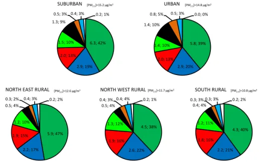
4.2.2 Annual average chemical composition of PM2.5 The annual average chemical composition of fine aerosol is depicted in Fig. 9 and shows a very similar pattern at the five sites, confirming the homogeneous feature of fine aerosol at the regional scale. The major chemical component is
or-ganic matter, accounting for 38 to 47 % of PMgrav
accord-ing to sites, and showaccord-ing a slightly higher contribution at the NER station for reasons given later on (Sect. 4.2.3). It is followed by nitrate (17–22 %), nss-sulfate (13–16 %) and ammonium (10–12 %) i.e. secondary inorganic aerosols. The highest SIA contributions are found at two rural sites (NWR and SOR) and are due to lower influences of local anthro-pogenic sources compared to the other locations. This leads to higher proportions of SIA even though mass concentra-tions remain approximately the same at the regional scale
(5.2 to 6.4 µg m−3). EC has a PM
2.5mass contribution of 4 to
10 %, and is about 3 times higher (in absolute concentrations) at URB and SUB than at rural sites because of its mainly lo-cal traffic source origin (Healy et al., 2012). Finally, dust and sea salts are minor components of fine aerosol in the region of Paris, representing 2 to 5 % and 3 to 4 % of its mass, respec-tively. The methodology developed to estimate the OC-OM conversion factor allows us to have a very small proportion of unaccounted mass (0 to 2 %). This overall chemical com-position is consistent with what is found in other European environments (Putaud et al., 2010, and references therein), exhibiting very high proportions of carbonaceous and sec-ondary inorganic aerosols.
4.2.3 Major chemical compounds of PM2.5
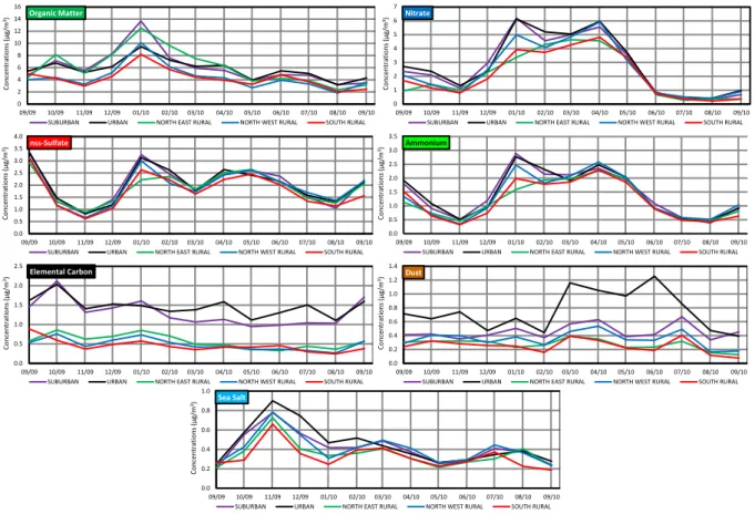
A detailed discussion of the spatial variability of each ma-jor chemical compound will now be given from the highest to the lowest contributor to fine aerosol mass concentrations (see Figs. 10 and 11). To begin with, OM shows fairly homo-geneous concentrations at the regional scale, on the whole duration of the project with good correlations between for
example SUB and URB (r2=0.82, slope = 1.08, n = 335),
NWR and URB (0.72, 0.79, 335) or NWR and SOR sites (0.73, 1.05, 351) and slopes fairly close to 1. As for PM, com-parable OM temporal variations are observed between sites,
M. Bressi et al.: A one-year comprehensive chemical characterisation of fine aerosol 7837
38 1
Fig. 8. Comparison between PM2.5 daily mass concentrations (gravimetric measurements) at the five
2
sites during the one-year period. 3
4
5
Fig. 9. Annual average chemical composition of PM2.5 (µg/m3; %) at the five sites from 11 September
6 2009 to 10 September 2010. 7 0 10 20 30 40 50 60 09/09 10/09 11/09 12/09 01/10 02/10 03/10 04/10 05/10 06/10 07/10 08/10 09/10 C onc en tr ations (µg /m 3)
SUBURBAN URBAN NORTH EAST RURAL NORTH WEST RURAL SOUTH RURAL
5.9; 47% 2.2; 17% 1.9; 15% 1.2; 10% 0.5; 4% 0.3; 2% 0.4; 3% 0.2; 2% NORTH EAST RURAL
OM Nitrate nss-Sulfate Ammonium EC Dust Sea salt Unaccounted mass [PM2.5]=12.6 µg/m3 4.3; 40% 2.2; 21% 1.8; 16% 1.2; 11% 0.4; 4% 0.3; 3% 0.3; 3% 0.2; 2% SOUTH RURAL [PM2.5]=10.8 µg/m3 4.5; 38% 2.6; 22% 1.9; 16% 1.3; 12% 0.5; 4% 0.4; 3% 0.4; 4% 0.2; 1% NORTH WEST RURAL[PM2.5]=11.7 µg/m3
5.8; 39% 2.9; 20% 2.0; 13% 1.4; 10% 1.4; 10% 0.8; 5% 0.5; 3% 0.0; 0% URBAN [PM2.5]=14.8 µg/m3 6.3; 42% 2.9; 19% 2.0; 13% 1.5; 10% 1.3; 9% 0.5; 3% 0.4; 3% 0.2; 1% SUBURBAN [PM2.5]=15.2 µg/m3 5.9; 47% 2.2; 17% 1.9; 15% 1.2; 10% 0.5; 4% 0.3; 2% 0.4; 3% 0.2; 2% NORTH EAST RURAL [PM2.5]=12.6 µg/m3
Fig. 9. Annual average chemical composition of PM2.5(µg m−3; %) at the five sites from 11 September 2009 to 10 September 2010.
39 1
Fig. 10. Daily mass concentrations (µg/m3) of the major chemical compounds of fine aerosol at the five sites from 11 September 2009 to 10 September 2010. 2 0 5 10 15 20 25 30 35 40 09/09 10/09 11/09 12/09 01/10 02/10 03/10 04/10 05/10 06/10 07/10 08/10 09/10 Organic Matter
SUBURBAN URBAN NORTH EAST RURAL NORTH WEST RURAL SOUTH RURAL 0 5 10 15 20 09/09 10/09 11/09 12/09 01/10 02/10 03/10 04/10 05/10 06/10 07/10 08/10 09/10 Nitrate
SUBURBAN URBAN NORTH EAST RURAL NORTH WEST RURAL SOUTH RURAL
0 2 4 6 09/09 10/09 11/09 12/09 01/10 02/10 03/10 04/10 05/10 06/10 07/10 08/10 09/10 Elemental Carbon
SUBURBAN URBAN NORTH EAST RURAL NORTH WEST RURAL SOUTH RURAL 0 2 4 6 8 10 12 09/09 10/09 11/09 12/09 01/10 02/10 03/10 04/10 05/10 06/10 07/10 08/10 09/10 nss-Sulfate
SUBURBAN URBAN NORTH EAST RURAL NORTH WEST RURAL SOUTH RURAL
0 2 4 6 8 09/09 10/09 11/09 12/09 01/10 02/10 03/10 04/10 05/10 06/10 07/10 08/10 09/10 Dust
SUBURBAN URBAN NORTH EAST RURAL NORTH WEST RURAL SOUTH RURAL 0 2 4 6 8 10 09/09 10/09 11/09 12/09 01/10 02/10 03/10 04/10 05/10 06/10 07/10 08/10 09/10 Ammonium
SUBURBAN URBAN NORTH EAST RURAL NORTH WEST RURAL SOUTH RURAL
Co n ce n tr ati o n s ( µ g/m 3) Co n ce n tr ati o n s ( µ g/m 3) Co n ce n tr ati o n s ( µ g/m 3) 0 1 2 3 4 09/09 10/09 11/09 12/09 01/10 02/10 03/10 04/10 05/10 06/10 07/10 08/10 09/10 Sea salt
SUBURBAN URBAN NORTH EAST RURAL NORTH WEST RURAL SOUTH RURAL
Co n ce n tr ati o n s ( µ g/m 3) Co n ce n tr ati o n s ( µ g/m 3) Co n ce n tr ati o n s ( µ g/m 3) Co n ce n tr ati o n s ( µ g/m 3)
Fig. 10. Daily mass concentrations (µg m−3)of the major chemical compounds of fine aerosol at the five sites from 11 September 2009 to 10 September 2010.
and very high levels can be followed by very low ones after only few days (e.g. on 27 and 29 January 2010, OM
con-centrations were 21.7–24.8 µg m−3 and 1.0–3.2 µg m−3
ac-cording to sites, respectively). This implies that a significant part of OM is either imported from outer regions of Paris, or spatially uniformly distributed over the region because
of similar primary emission sources. The latter argument is very unlikely because primary emission sources of OM, such as wood burning (WB) (Puxbaum et al., 2007, and refer-ences therein) and traffic (Thorpe and Harrison, 2008; Pio et al., 2011) are thought to be rather local and site-dependent. In fact concerning WB, good correlations between OM and
40 1
Fig. 11. Monthly mass concentrations (µg/m3) of the major chemical compounds of fine aerosol at the five sites from 11 September 2009 to 10 September 2 2010. 3 0 2 4 6 8 10 12 14 16 09/09 10/09 11/09 12/09 01/10 02/10 03/10 04/10 05/10 06/10 07/10 08/10 09/10 Organic Matter
SUBURBAN URBAN NORTH EAST RURAL NORTH WEST RURAL SOUTH RURAL 0 1 2 3 4 5 6 7 09/09 10/09 11/09 12/09 01/10 02/10 03/10 04/10 05/10 06/10 07/10 08/10 09/10 Nitrate
SUBURBAN URBAN NORTH EAST RURAL NORTH WEST RURAL SOUTH RURAL
0.0 0.5 1.0 1.5 2.0 2.5 3.0 3.5 4.0 09/09 10/09 11/09 12/09 01/10 02/10 03/10 04/10 05/10 06/10 07/10 08/10 09/10 nss-Sulfate
SUBURBAN URBAN NORTH EAST RURAL NORTH WEST RURAL SOUTH RURAL 0.0 0.5 1.0 1.5 2.0 2.5 3.0 3.5 09/09 10/09 11/09 12/09 01/10 02/10 03/10 04/10 05/10 06/10 07/10 08/10 09/10 Ammonium
SUBURBAN URBAN NORTH EAST RURAL NORTH WEST RURAL SOUTH RURAL
0.0 0.5 1.0 1.5 2.0 2.5 09/09 10/09 11/09 12/09 01/10 02/10 03/10 04/10 05/10 06/10 07/10 08/10 09/10 Elemental Carbon
SUBURBAN URBAN NORTH EAST RURAL NORTH WEST RURAL SOUTH RURAL 0.0 0.2 0.4 0.6 0.8 1.0 1.2 1.4 09/09 10/09 11/09 12/09 01/10 02/10 03/10 04/10 05/10 06/10 07/10 08/10 09/10 Dust
SUBURBAN URBAN NORTH EAST RURAL NORTH WEST RURAL SOUTH RURAL
Co n ce n tr ati o n s ( µ g/m 3) Co n ce n tr ati o n s ( µ g/m 3) Co n ce n tr ati o n s ( µ g/m 3) Co n ce n tr ati o n s ( µ g/m 3) Co n ce n tr ati o n s ( µ g/m 3) Co n ce n tr ati o n s ( µ g/m 3) 0.0 0.2 0.4 0.6 0.8 1.0 09/09 10/09 11/09 12/09 01/10 02/10 03/10 04/10 05/10 06/10 07/10 08/10 09/10 Sea Salt
SUBURBAN URBAN NORTH EAST RURAL NORTH WEST RURAL SOUTH RURAL
Co n ce n tr ati o n s ( µ g/m 3)
Fig. 11. Monthly mass concentrations (µg m−3)of the major chemical compounds of fine aerosol at the five sites from 11 September 2009 to 10 September 2010.
levoglucosan (not shown here) at the NER site during cold days assert the presence of a local source, explaining higher OM concentrations at this site, and less satisfactory correla-tions with the other rural sites (e.g. for NER plotted against
SOR sites, r2=0.55, slope = 1.46, n = 330). Moreover,
dur-ing low BLH days, clearly higher OM concentrations are found at URB, SUB and NER sites compared to NWR and SOR ones (e.g. 31 October 2009) that can be explained by the enhancement of local WB sources. It is however likely that a part of WB aerosols is also due to mid-range trans-port as suggested by the comparison of levoglucosan levels between sites and as reported for biomass burning (includ-ing WB) in other regions of the world (Niemi et al., 2005, 2009; Stohl et al., 2007; Mochida et al., 2010). It is worth-while noting that given the large expected emissions associ-ated with the Larger Urban Zone of Paris, it could reasonably be assumed that the OM spatial homogeneity observed in our study is the consequence of secondary formation processes of precursor emissions in the Paris region. The time needed for gas-to-particle conversion would explain the observed spatial variability of OM, which would be supported by the high ob-served fOC-OM values. Nevertheless, modelling and exper-imental studies conducted during the EU-MEGAPOLI sum-mer and winter field campaigns by Crippa et al. (2013),
Freu-tel et al. (2013) and Zhang et al. (2013) do not support this as-sumption. Conversely, the aforementioned studies report that (i) OA is mostly controlled by mid- or long-range transport (Crippa et al., 2013), (ii) the influence of the Paris emission plume onto its surroundings is rather small for primary or-ganic aerosols (Freutel et al., 2013) and (iii) the highest OA levels are due to the advection of SOA from outside Paris (Zhang et al., 2013). To conclude, in the region of Paris, OM is therefore mainly imported by mid- or long-range transport, although local sources such as traffic and wood burning also contribute to its atmospheric concentrations.
SIA including nitrate, nss-sulfate and ammonium also shows very good site-to-site covariations during this study (Figs. 10 and 11). As already mentioned in Sect. 4.1.2, SIA concentrations highly depend on air mass origins and temperatures, and are mainly due to transboundary mid- or long-range transport from countries located east of France (Bessagnet et al., 2005; Sciare et al., 2010, 2011). However,
local emissions of precursor gases such as NOx, NH3 and
SO2can partly explain the discrepancies observed between
sites for nitrate and ammonium concentrations, and to a lower extent for nss-sulfate (Figs. 9, 10 and 11). In fact, when focusing again on the end of October (that was under low BLH conditions), nitrate shows a clear gradient exhibiting
![[PDF] Initiation au développement Qt sur les sockets | Cours informatique](data:image/gif;base64,R0lGODlhAQABAIAAAP///wAAACH5BAEAAAAALAAAAAABAAEAAAICRAEAOw==)