Design, optimization, and performance of an adaptable aircraft manufacturing architecture

Design, Optimization, and Performance

of an

Adaptable Aircraft Manufacturing Architecture

Tony S. Tao

B.S. The Pennsylvania State University, 2010

S.M. Aeronautics & Astronautics, Massachusetts Institute of Technology, 2012

Submitted to the Department of Aeronautics & Astronautics in Partial Fulfillment of the Requirements for the Degree of

Doctor of Philosophy

Massachusetts Institute of Technology

-A-tgttsf-2&918; LeptemberQ

2.IN3

2018 Massachusetts Institute of Technology. All rights reserved.

Signature redacted

S

OCT 0 2018

LIBRARIES

Signature redacted

ignature redacted

Mark Drela Thesis Committee, Professor of Aeronautics & Astronautics, MIT

Signature redacted______

Olivier de Weck Thesis Committee, Professor of Aeronautics & Astronautics, MIT

Signature redacted

Hamsa Balakrishnan Chair, Department Graduate Committee, MIT Author:

Design, Optimization, and Performance

of an

Adaptable Aircraft Manufacturing Architecture

Tony S. Tao

Submitted to the Department of Aeronautics and Astronautics on August 23, 2018

in partial fulfillment of the requirements of the Degree of Doctor of Philosophy

in Aeronautics and Astronautics

Abstract

The cost and time required to develop aircraft have grown strongly over time, to the point where aircraft have become prohibitively expensive and are outpaced by ever-evolving mission needs. To address this problem, this thesis presents and explores an aircraft platform architecture called "Adaptable Aircraft Manufacturing" or "AAM", which features common tooling geometry that enables the creation of any composite aircraft (within a reachable subspace) on demand. To prove the feasibility of this architecture, a family of aircraft was constructed using a single set of AAM tooling. This thesis also optimizes the AAM geometry and quantifies the inefficiencies incurred by its adoption. This family optimization problem is both logically and computationally complex since the constraints AAM places between the variants cannot be prescribed by the designer, but arise as a result of the optimization gradients that exist between variants. A sequential-process framework which clarifies the relations and points of adjustability available in aircraft manufacturing is presented. A signomial-programming (SP) aircraft optimization code that is capable of simulating the inefficiencies generated by the AAM geometry was developed. The SP

mathematical structure and the GPkit codebase were selected due to their compatibility with the constraint-heavy geometric rules that describe AAM and for the rapid speed of computation, which is necessary due to the scale of the optimization problem. To quantify the performance of AAM, a series of explorations are conducted whereby the performance of an AAM-family of aircraft is compared against a fleet of Individually-Optimal (IO) aircraft. These explorations are conducted along the axes of payload size, cruise speed, mission scope, and market bias to gain an understanding of how (and by how much) the AAM constraints affect both the performance and the geometry of the aircraft it produces. The results show that, for total-mission-cost-minimizing fleets of three designs each, the AAM fleet is between 10 and 20% more costly, but only require between 30% and 80% the tooling as an 10 fleet.

Thesis Supervisor: R. John Hansman

For Percy and Orion.

Anything worth doing is worth doing badly.

- GK Chesterson

All progress depends on the unreasonable man.

- George Bernard Shaw

If it doesn't get done in a hurry, it doesn't get done at all.

Table of Contents

1 In tro d u ctio n ... 13

1 .1 M o tiv a tio n ... 13

1.2 Tooling and Platforms... 14

1.2.1 Tooling as a driver of cost and schedule ... 14

1.2.2 Product platforms... 16

1.3 Prior W ork in Family Optimization Computation... 18

1.4 Adaptable Aircraft M anufacturing: Goals and Thesis Layout... 19

1.4.1 Thesis structure ... 19

2 Adaptable Aircraft M anufacturing (AAM )... 20

2.1 Com posite Aircraft M anufacturing... 20

2.2 Geom etry of Adaptable Aircraft M anufacturing... 23

2.2.1 Com m on m olds and adjustable-layup ... 23

2.2.2 Adjustable-layup applied to wings and tails ... 24

2.2.3 Adjust able-layup applied to fuselages ... 27

2.2.4 Integration challenges in AAM structures... 28

2.3 AAM Proof of Concept: "FAST" Project ... 28

2.3.1 Lessons from FAST and the problem of designing AAM fam ilies... 30

2.4 W ay Forward ... 31

3 Robustness and Adaptability Framework... 32

3.1 Classical Optim ization Form ulation... 32

3.1.1 Exam ple of classical optimization: basic airfoil design problem ... 33

3.2 Uncertainty, Robust Designs, and Robustness... 34

3.2.1 Robust designs and robustness... 34

3.2.2 Robustness in the airfoil design example... 34

3.2.3 Asym metry in robustness ... 36

3.3 Passive and Active Robustness and Adaptability... 36

3.3.1 Adaptable robustness in the airfoil design exam ple ... 36

3.3.2 Costs of adaptability ... 38

3.3.3 Rate of uncertainty and adaptability ... 38

3.4 Fram ework to Describe Adaptability Process Sequences ... 39

3.4.1 "Process Sequence" framework... 39

3.4.2 Asset space m apping abstraction ... 40

3.4.4 Fram ework applied to the airfoil exam ple... 41

3.4.5 Uncertainty, robustness, and adaptability within framework ... 41

3.5 Fram ework Applied to Aircraft M anufacturing Chains ... 42

3.6 Representing Other Designs ... 43

4 AAM Perform ance Quantification ... 45

4.1 Baseline M ission Overview ... 45

4.1.1 Baseline driving requirem ents... 46

4.2 Total System Cost M etric ... 47

5 Geom etric and Signom ial Program m ing ... 48

5.1 Com putational Challenges in Designing Aircraft Fam ilies... 48

5.2 Geometric Program m ing ... 48

5.3 Signom ial Program m ing ... 49

5.4 Coding Setup for Optim ization Problem ... 50

6 M o d e ls ... 5 1 6.1 Fitting Procedure for Com plex Data... 51

6.2 Atm ospheric M odels ... 52

6.3 Aircraft configuration ... 52

6.4 Airfram e M aterial Assum ptions ... 53

6.5 Com m on M olding Geom etry M athem atics... 54

6.5.1 W ings and tails... 54

6.5.2 Fuselages ... 56

6.6 W ing M odels... 57

6.6.1 W ing aero: lift m odel... 58

6.6.2 W ing aero: induced drag m odel... 58

6.7 W ing Discretization for Load and Response Structures... 59

6.7.1 W ing aero: airfoil perform ance m odel ... 60

6.7.2 W ing bending loads m odel ... 61

6.7.3 W ing bending structure: spar ... 63

6.7.4 W ing torsion loading cases ... 64

6.7.5 W ing structure: torsion box ... 66

6.7.6 Torsion stiffness constraint... 66

6.7.7 W ing root joiner m ass m odel... 67 6 .8 T a il M o d els ... 6 8 6 .8 .1 T a il sizin g ... 6 8

6.9 W ing and Tail Com m onality Constraints ... 69

6.10 Fuselage M odels ... 70

6.10.1 Fuselage Drag ... 70

6.10.2 Fuselage pitch and yaw bending loads ... 72

6.10.3 Fuselage roll loads ... 74

6.10.4 Fuselage com m onality constraints... 75

6.11 Propulsion M odels ... 76

6.11.1 Takeoff propulsion m odel ... 76

6.11.2 Cruise power m odel ... 77

6.11.3 Cruise range m odel... 77

6.11.4 Engine m ass m odel... 77

6.12 Aircraft Balance ... 78

6.13 Aircraft Optim ization Code Exam ple Outputs ... 79

7 AAM Explorations and Discussion ... 80

7.1.1 Scope vs. perform ance ... 81

7.2 Payload Explorations ... 81

7.2.1 Exploration 1: Fam ily perform ance vs. payload scope ... 83

7.2.2 Exploration 2: Fam ily and variant Perform ance vs m arket bias ... 88

7.2.3 Exploration 3: Fam ily perform ance vs scope and m arket bias... 90

7.2.4 Exploration 4: Com m on wings and tails but unique fuselages ... 91

7.3 Cruise Speed Explorations... 94

7.3.1 Cruise speed exploration setup ... 94

7.3.2 Exploration 5: Cruise speed... 95

8 Conclusion and Recom mendations... 98

8.1 Conclusion ... 98

8.2 AAM Usage Recom m endations ... 98

8.3 Future W ork Recom m endations... 98

9 W orks Cited ... 101

10 Appendix ... 105

10.1 Atm ospheric properties...105

List of Figures

Figure 1.1: US combat aircraft unit price over time [1] with inflation overlay... 13

Figure 1.2: Years from program start to initial operational capability over time [2]... 13

Figure 1.3: Max, median, and mean age of designs in Air Force service [3] ... 14

Figure 1.4: Boeing data for cost over time for the development of a large commercial jet [4]... 15

Figure 1.5: Trends in composite material use in aircraft [1] ... 16

Figure 1.6: Boeing 737NG Family ... 17

Figure 1.7: Antares 20E sailplane [5]... 17

Figure 1.8: Extended wing molding strategy for the Antares 18S/T and 20E sailplanes [6] ... 18

Figure 1.9: BW B structural breakdown [71 ... 18

Figure 2.1: Bagged layup schematic ... 20

Figure 2.2: W ing skin molds for the Boeing 777X [9]... 21

Figure 2.3: Cirrus SR22 fuselage molding [10]... 21

Figure 2.4: Boeing 787 nose section production [11]... 22

Figure 2.5: Adjustable-layup strategy ... 23

Figure 2.6: Cylindrical abstraction of primary aircraft structural geometries... 23

Figure 2.7: Layout of conventional wing construction ... 24

Figure 2.8: Sailplane wing internal component integration... 24

Figure 2.9: Detailed wing structure of Airbus ALCAS wing box [12]... 25

Figure 2.10: Common wing tooling concept ... 25

Figure 2.11: Spar mold shift to compensate for shell thickness... 26

Figure 2.12: W ing planform comparison between three airliners ... 26

Figure 2.13: W ing planform comparison between three large UAVs... 27

Figure 2.14: Applying adjustable-extent to fuselages allows the production of a variety of lengths... 27

Figure 2.15: Three aircraft constructed from common tooling (left to right: A,B,C) ... 28

Figure 2.16: W ing commonality between FAST A and B... 29

Figure 2.17: Molds for FAST project (tail: left, wing: right) ... 29

Figure 2.18: FAST A (spine in white box)... 30

Figure 3.1: Airfoil example: baseline performance... 33

Figure 3.2: Airfoil example: small uncertain CI scope ... 35

Figure 3.3: Airfoil example: large uncertain Cl scope... 35

Figure 3.4: Airfoil example: large uncertain Cl range causing infeasibility ... 36

Figure 3.5: Airfoil example: adaptable-robustness of a2 ... 37

Figure 3.6: Airfoil example: adaptable-robustness of al... 38

Figure 3.7: Variable-space mapping abstraction ... 40

Figure 3.8: Unit "block" of PSM ... 41

Figure 3.9: PSM for simple, non-adaptable airfoil in lift-drag optimization problem ... 41

Figure 3.10: PSM for flapped airfoil in lift-drag optimization problem... 41

Figure 3.11: PSM for baseline manufacturing-through-operation chain... 42

Figure 3.12: PSM for Adaptable Aircraft Manufacturing ... 42

Figure 3.13: PSM for AAM with aircraft reconfigurability ... 43

Figure 3.14: PSM for an example building-block aircraft platform... 44

Figure 4.1: AAM performance quantification procedure ... 45

Figure 4.3: Assumed aircraft configuration ... 46

Figure 6.1: GP-compatible fitting procedure... 51

Figure 6.2: Atmospheric property ratios ... 52

Figure 6.3: Assumed aircraft structure and geometry... 53

Figure 6.4: Trapezoidal wing geometry ... 54

Figure 6.5: W ing design spaces as a function of taper angle and taper ratio... 55

Figure 6.6: Fuselage geometry... 56

Figure 6.7: Commonality scheme for fuselages... 56

Figure 6.8: Induced drag simulated data (points) and GP-model fits (lines)... 59

Figure 6.9: Discretized spar model schematic for wings and tails... 60

Figure 6.10: GP-compatible airfoil model for NACA 24xx airfoils [23]... 60

Figure 6.11: Bending moment ratio vortex-lattice and GP-model... 61

Figure 6.12: Notional nondimensionalized wing bending distribution as a function of taper ratio... 62

Figure 6.13: W ing spar bending stiffness limit model ... 62

Figure 6.14: Radius of curvature vs wing deflection ratio for b=2 ... 63

Figure 6.15: W ing spar model ... 63

Figure 6.16: M aximum nose-down torsion case... 65

Figure 6.17: M aximum nose-up torsion case ... 65

Figure 6.18: W ing box torsion model... 66

Figure 6.19: W ing joiner mass estimation schematic ... 67

Figure 6.20: Fuselage geometry variables... 70

Figure 6.21: Sample fuselage CFD plot ... 71

Figure 6.22: GP modeling fitment for fuselage drag (fit data vs CFD data) ... 72

Figure 6.23: Fuselage load schematic (bending)... 73

Figure 6.24: Roll force input model... 74

Figure 6.25: Fuselage load schematic (torsion) ... 75

Figure 6.26: Aircraft weight balance schematic... 78

Figure 6.27: Code output for baseline mission ... 79

Figure 7.1: AAM performance evaluation procedure... 80

Figure 7.2: Payload Explorations map ... 82

Figure 7.3: Fleet performance ratios vs scope factor ... 83

Figure 7.4: Spay=1, Z =1 AAM and IO fleet comparison ... 84

Figure 7.5: Spay=3, Z=1 AAM and IO fleet comparison ... 84

Figure 7.6: Spay=5, &=1: AAM and IO fleet comparison ... 85

Figure 7.7: Spay=10, &=1 AAM and 10 fleet comparison ... 86

Figure 7.8: Empty mass ratio between AAM and IO vs scope ... 87

Figure 7.9: Aircraft mass vs payload carried (illustrations on left are to-scale) ... 87

Figure 7.10: AAM optimal aircraft as & is varied, vehicles are to-scale... 88

Figure 7.11: Relative performance of AAM variants against 10 vs & ... 88

Figure 7.12: Relative mold area vs 4 ... 89

Figure 7.13: Aircraft empty mass vs. payload carried, for S-sweeps and Z =1 and 0.2 ... 90

Figure 7.14: Full and partial-AAM and IO aircraft for Spay = 5, 4 = 1... 91

Figure 7.15: Empty mass of variants #1 and #3 vs payload carried for full and partial AAM... 92

Figure 7.16: Fleet performance ratios for full-AAM and partial AAM vs scope... 93

Figure 7.18: Result of cruise-speed-varying mission set with Sspeed = 5... 95 Figure 7.19: Taper angle comparison between AAM and IO fleets... 97

1

INTRODUCTION

This chapter introduces the problem of cost and development duration in aircraft design and manufacturing, background on tooling and platforms, and the goals and layout of this thesis.

1.1 Motivation

The cost of aircraft and the time required to develop them have grown strongly over time, as shown in Figure 1.1. The unit cost of aircraft has risen approximately 9% yearly since 1975, exceeding all other measures of inflation [1]. 1,000 'U S 100 10 1970 * F/A-18E/F - F/A-18A/B/CID A F-14A/D X F-15A/B/CiD/E 0 F-16A/B/C/D X VV ase 0 F-5E/F V F-22 _01 0

*

Figure 1.1: US combat aircraft unit price over time [11 with inflation overlay

Whereas other industries such as automotive engineering have seen an increase in development speed, aircraft development (both military and commercial) have become increasingly slow since the post-WWII period, as shown in Figure 1.2 from DARPA [2].

M25 C 015 5 F-35' F-22 C-2 8 ... "U FoE F-15 - 0 .*F-85 A& 4A W M 20M 2015 2025

Year of 10414al Operatleal Capabilifty

Distribution Statement 'A" (Approved for Public Rease, Distribution Unlimited)

Figure 1.2: Years from program start to initial operational capability over time [21

The combination of high cost and slow development has significant implications for satisfying new

missions. First, many aircraft development projects are abandoned due to lack of funding. Second, even if an aircraft project survives to completion, the development can take so long that the mission context will have changed by the time the aircraft is ready for service. For example, the request-for-proposals for the F-22 Raptor was issued in 1986, and the aircraft entered service in 2005: 19 years later [2]. Over that period, the nature of aerial warfare had changed from the air supremacy of the Cold War to asymmetric and electronic warfare in the Middle East, and many of the F-22's features remain unused.

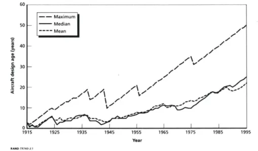
These effects may also be quantified at the fleet level. Figure 1.3 from the RAND Corporation shows the trends for design-age of US Air Force vehicles over time [3].

60 -- Maximum 50 - - Median ---- Mean S40 230

~

Figure 1.3: Max., median. and mean age of designs in Air Force service .3/

As Figure 1.3 shows, the design-age of aircraft in the US Air Force is rising steadily, and aircraft require constant retrofitting and modernization programs to remain current. Retrofitting existing aircraft for new missions results in suboptimal matching between designs and missions since the base airframes carry all the original tradeoffs into their new roles.

In summary, aircraft development is often prohibitively expensive and is outpaced by ever-changing mission needs. Decreasing aircraft development cost and increasing development speed would provide benefits - for both individual projects and the fleet as a whole. This thesis explores one novel approach to achieving this goal.

1.2 Tooling and Platforms

While much of the cost and schedule for new aircraft is the result of increased use of software and electronics, hardware manufacturing still represents a large investment for new aircraft and is an area of opportunity due to its potential for commonality.

1.2.1 Tooling as a driver of cost and schedule

"Tooling" is a generic term for the hardware necessary to convert raw materials into a final product, and is one of the main drivers of aircraft development cost and duration. Depending on the material of the part being constructed, tooling may be comprised of molds, dies, jigs, fixtures, or other devices. In this

usage, "tooling" is distinct from "machines" such as mills and lathes which, without alteration, can produce a multitude of components.

Tooling is a necessary precursor to producing airframe components. For the vast majority of vehicles, the design and production of tooling is orders of magnitude more expensive and time-consuming than

producing a single unit. For example, analysis of Boeing data by Markish in Figure 1.4 shows the normalized labor hours vs. the normalized development time for one large commercial jet program [4].

QA

abs

_{*Baseline QA}

*Baseline Dev. Labs

0

*Baseline Tool Fab

0 Baseline

Tool Design

0 0Baseline M.E. C 0 Baseline Engr. 0 e Basefine Engr. 0

non-dimensional time

Figure 1.4: Boeing data for cost over time for the development of a large commercial jet|4 The study shows that tooling design (yellow) and fabrication (teal) accounts for roughly 45% of development cost and dominates labor-hours for 50% of the schedule [4]. During a typical design-to-manufacture schedule for an airliner, tooling design and fabrication would take approximately 4 years. In contrast, the production of a single unit of a finalized design only takes a few weeks.

Most tooling is specific to a single aircraft design's geometry, so even subtle changes in an aircraft's external lines (such as airfoil tweaks) requires the creation of new tools. As a result, design changes late during development usually involve substantial growths in cost and schedule.

The prevalence of tooling-driven project cost and schedule is likely to grow. According to a study by the RAND Corporation, much of the price increase in today's aircraft stems from the desire for higher

performance, which is partly achieved through the increased use of advanced materials such as composites (as shown in Figure 1.6) [1].

Trend in Composite Material Use in Aircraft, 1967 to 2000 60 V-22 FSD + Air Force 50 -

_a

e

RAND MG696-. I

Figure 1.5: Trends in composite material use in aircraft /1/

Composite materials, unlike metals, cannot be machined from billet or pressed from sheet stock. Instead, they must be molded. Manufacturing composite airframes concentrates development cost and duration into molds, fiber-placement machines, and autoclaves.

1.2.2 Product platforms

A product "platform" strategy is one in which some common technology or components are shared between "variants" within a product "family". Each variant serves a different market or mission need, but since they share a subset of their requirements, these common requirements may be fulfilled with common components.

Designing for commonality between variants introduces constraints and reduces the available design space. Therefore, commonality almost invariably reduces the performance of each variant (in comparison to what may be achieved individually). In return, product platforming provides several benefits:

Firstly, commonality can reduce development cost and duration for the family as a whole. Design and tooling costs for common components can be amortized over a large number of units, and economies of scale and the learning curve effect reduce the costs associated with common components. The time spent developing common components does not have to be repeated for additional variants.

Secondly, once the platform's manufacturing architecture has been constructed, new variants may be developed more rapidly and at lower cost than starting from scratch.

1.2.2.1 Platform architectures

For the purposes of this work, the "architecture" of a platform is defined as the manner in which the variants share commonality. "Architecture" is akin to the "configuration" of the platform, and does not necessarily specify any of the dimensions or mechanical details of the variants.

Most hardware platforms use a "building-block" architecture in which some components are interchangeable between variants in the family. One example of such an architecture would be an automaker's range of cars that share the same engine and transmission. Another example is a set of electric motors, batteries, and control boards that are common in a line of power tools.

1.2.2.2 Platform architectures in aeronautical engineering

Most modern airliners (such as the Boeing 737NG family shown in in Figure 1.6) are designed using a building-block architecture in which wings, tails, and sections of the fuselage are common between variants while segments called "plugs" are added to the fuselage in front and behind the wing to increase passenger capacity. This strategy is often called fuselage "stretching".

am~ $$ae wgs soe *o so ag .M I Ur-0EM1 N377 FAMILY

Figure 1.6: Boeing 737NG Family

This "stretching" architecture is used by both the Boeing 737 family and Airbus A320 family, but these two families are incompatible due to differences in the specific dimensions of their system interfaces. A less-common, adjustable-tooling-based platform architecture is used in the Antares 18S/T and 20E sailplanes (Figure 1.7). Instead of installing additional sections during aircraft assembly, to manufacture the longer-wingspan version, a 1-meter, constant-chord mold section is placed between the outboard wing and the root (Figure 1.8). The resulting wings are structurally identical outboard of the red segment.

Figure 1.7: Antares 20E sailplane

f51

~-~m

EV.

The Boeing and Antares examples in the section above have different architectures: whereas the Boeing 737 variants share the same wings and tails, the Antares sailplane variants share the same fuselages. In both, however, the architectures are varied in primarily one dimension - fuselage length in the case of the Boeing architecture and wingspan in the Antares architecture.

1.3 Prior Work in Family Optimization Computation

The idea of sharing airframe components between variants has been explored by many researchers in the past; two of these efforts are highlighted below.

In 2003, Willcox and Wakayama published their study on the simultaneous optimization of two blended-wing-body (BWB) aircraft that carry different numbers of passengers. In their design, the inner wing, outer wing, and winglets (as shown in Figure 1.9) are common between the variants while the

centerbodies are permitted to be different. This research highlighted the scaling and numerical conditioning issues that occur when multiple vehicles are optimized simultaneously. [7]

outer ving

inner wing g

Fig. 3 Modular struclural breskdown of BWlL Figure 1.9: BWB structural breakdown [71

In 2016, Jansen and Perez published a study investigating the optimization of a family of aircraft for a range of markets, characterized by both passenger count and flight range. Discrete and binary decision variables are used to control aircraft design. To deal with the mixed-continuous/discrete nature of this optimization problem, the researchers used a Particle-Swarm-Optimization (PSO). [8]

In these previous works, the architecture is designed such that a component of the aircraft (a wing, tail, fuselage segment, etc.) is either common or unique. In contrast, the work in this thesis focuses on an architecture that permits continuous-variability in the geometry of aircraft components.

1.4 Adaptable Aircraft Manufacturing: Goals and Thesis Layout

This thesis explores a platform architecture called "Adaptable Aircraft Manufacturing" (or "AAM" for short). AAM is designed to reduce aircraft manufacturing cost and duration for composite aircraft while providing designers a large degree of freedom in important aerodynamic and structural variables so that a large range of missions may be accomplished without retooling.

1.4.1 Thesis structure

First, Chapter 2 discusses the physical design of AAM, its compatibility with composite structures, the degrees of freedom each variant can have, and the constraints it places between variants. This chapter also describes the FAST project, which acts as a physical proof-of-concept to demonstrate the feasibility of the architecture. Chapter 2 concludes by discussing the challenges of designing an AAM family and sets the scope for the remainder of this work, which is to quantitatively explore the performance tradeoffs generated by AAM.

To evaluate the architecture's performance, it is necessary to optimize the families enabled by the architecture. To organize this type of adaptable-robust optimization problem, Chapter 3 presents a framework which defines and clarifies the connections and dependencies inherent in the design of the full lifecycles of aircraft platforms - from tooling, production, vehicle, through operation to satisfy a variety of missions.

Chapter 4 presents the AAM performance quantification procedure.

Like many adaptable-robust optimization problems, the design of AAM families requires the optimization of a complex web of relations consisting of thousands of variables. Chapter 5 discusses the choice of using Geometric and Signomial Programming.

Since Signomial Programming is a relatively new system for the optimization of aircraft, many new models and relations were developed to capture the tradeoffs inherent in AAM. Chapter 6 presents these models.

Chapter 7 presents a series of "Explorations" into the performance of AAM as it responds to mission scenarios.

Chapter 8 presents a discussion of the results, recommendations about how AAM might be useful to aircraft development companies, and recommends the direction of future development.

2 ADAPTABLE AIRCRAFT MANUFACTURING

(AAM)

"Adaptable Aircraft Manufacturing" (AAM) is a platform architecture1 for composite aircraft in which a single set of molds is used to manufacture the primary structures of multiple variants. The degrees of freedom within the architecture enables designers to adjust the aircraft's geometry during manufacturing, which allows a variety of missions to be accomplished without retooling.

To understand how this architecture functions, it is first necessary to understand conventional composite manufacturing. This chapter first describes conventional composite manufacturing processes. From this baseline description, the strategies used in AAM, its degrees of freedom, and its constraints are described.

For the purposes of this work, conventional tube-and-wing designs shall be considered, though the concepts presented herein are scalable to other vehicle configurations as well, such as flying wings or blended-wing-bodies.

2.1 Composite Aircraft Manufacturing

Advanced composites (fiberglass, carbon fiber, aramid, or other fibers bonded within an epoxy or other polymer matrix) are used in aircraft for their high strength- and stiffness-to-weight ratios, ability to provide tailored orthotropic material properties, compatibility with complex three-dimensional shapes, and other properties. Unlike sheet metals (which can be bent and shaped with jigs and ribs, machined, or forged into shape), constructing composite structures requires tooling investment in the form of molds. The molds are necessary to support and shape the plies during the layup process and constitute the largest per-design tooling investments for the production of composite airframes.

The most common method for molding components is a "bagged layup". This technique is ubiquitous in both small and large aircraft due to its compatibility with complex part geometries, tolerance to imperfect ply placement, and uneven ply thicknesses. In addition, a minimum of one mold may be used to produce a single part. Figure 2.1 below shows a schematic and layer order for a typical bagged layup.

Layup schedule Untooled surface Sag Breather Peelpl Mold-relese 4

Precise, tooled surface Mold

Pressure -. Vacuum

Figure 2.1: Bagged layup schematic

1

As shown in Figure 2.1, the interface between the mold and the plies forms the "tooled surface", which is precisely controlled during mold manufacturing. The external surfaces of wings, fuselages, and tails are almost invariably formed by this tooled surface while the "untooled surface" is typically exposed to the inside of the structure where surface finish is inconsequential. A mold-release (commonly a spray-on coating or wax) is applied to enable the removal of the cured layup from the mold. For example, Figure 2.2 below shows the wing skin mold for the Boeing 777X [9].

Figure 2.2: Wing skin molds for the Boeing 777X /91

Soft, uncured plies of composite material are then laid on top of the molds either by hand or by layup machines. The layout and order of layup components are often referred-to collectively as the "layup schedule". The layup frequently includes multiple types of fiber materials, cores to form sandwich panels, hard points, and other components as exemplified in Figure 2.3. The green-tinted sections are fiberglass laminate while the orange-tinted sections reveal the cores that stiffen the shell.

Peel ply and breather fabric are then layered on top of the layup. The peel ply enables the separation of the layup plies from the breather. The interface between the peel ply and the layup forms the "untooled surface" which is significantly less precise in dimension than the tooled surface due to variations in ply or core thicknesses. The mechanical compliance of the peel ply, breather, and bag ensures compression during the curing process despite these variations.

In preparation for the curing process, air is removed from the bag using a vacuum pump. Figure 2.4 below shows the peel ply, breather, and bag layers being applied to the nose section of a Boeing 787.

. . .. . . .. .

Figure 2.4: Boeing 787 nose section production /111

For a composite layup to achieve its maximum strength, pressure and heat must be applied (using an autoclave) to compress the plies together and cure the epoxy. The combination of internal vacuum and external pressure minimizes the presence of voids in the layup, squeezes out excess epoxy, and minimizes the interlaminar distance. The layup assembly is heated and cooled following a temperature profile designed to flow and then solidify the epoxy and lock the fibers together. The interaction of fibers and hardened matrix generates the part's strength, stiffness, and other properties.

After removing the parts from the molds, post-processing steps such as cutting, fastening, and bonding may be used to finalize and join parts together to create aircraft components. Jigs can be used to align components for assembly, or parts may be self-aligning due to their geometry.

2.2 Geometry of Adaptable Aircraft Manufacturing

2.2.1 Common molds and adjustable-layup

Unlike conventional platform architectures that reuse whole components (such as the wing or tails) between variant vehicles, AAM is based on an "adjustable-layup" strategy that may be applied during the production of every component. The adjustable-layup concept is illustrated in Figure 2.5.

Adjustable-layup

Adjustable-schedule

Adjustable-extent

Mold

Figure 2.5: Adjustable-layup strategy

As shown in the figure, layup" is composed of two separate degrees of freedom: "adjustable-extent" and "adjustable-schedule". These changes in the layup procedure may be achieved either manually by technicians or by reprogramming the machines in automated fiber-placement systems.

"Adjustable-extent" refers to the degree of freedom that a layup may terminate before the end of the mold in the spanwise axis (for wings and tails) or lengthwise axis (for fuselages). This degree of freedom

leverages the fact that standard wing, tail, and fuselage structures can be described as cylindrical shells of arbitrary cross-section with axial stiffeners, as shown in Figure 2.6. Terminating and capping structures at stations along the extruded axis produces components compatible with the loads on these structures. Instead of having discrete breakpoints, the extent of the layup may be controlled as continuous variables.

Cylinder of arbitrary cross-section

Extruded axis

Fuselages, booms, etc. Wings, tails

Figure 2.6: Cylindrical abstraction of primary aircraft structural geometries

"Adjustable-schedule" refers to the degree of freedom in the position, composition, and number of plies that may be placed during the layup process. This degree of freedom leverages the fact that the peel ply,

breather, and bag layers are compatible with any number and composition of plies a designer chooses during manufacturing in a bagged layup.

The sections below describe AAM's compatibility with typical aircraft structures and the degrees of freedom and constraints it generates at both the tooling and vehicle production stages.

2.2.2 Adjustable-layup applied to wings and tails

Discussions in this section regarding "wings" also apply to tails. For the purposes of this work, trapezoidal planform geometries are considered. While other planforms are possible, a trapezoidal planform is

reasonable for most aircraft and is illustrative of the concept.

AAM's adjustable-layup strategy may be applied to the primary load-carrying structures (skins, spars, and shear webs) of conventional hollow wing designs since these components are composed of slender, tapered elements that run spanwise from the wing root to the wing tip (as shown in Figure 2.7).

Upper mold

Upper skin Sparcap

- Wing box

Lower skin - Shear web(s)

Spar cap Lower mold

Figure 2.7: Layout of conventional wing construction

Examples of this construction technique may be seen in Figure 2.8 (a sailplane wing prior to final closure).and in Figure 2.9 (the ALCAS wing design from Airbus [121).

GCOW Rib

LJ"'Cve

Sie Sdy

Figure 2.9: Dctailed wing structure of Airbus ALCAS wing box 1121

Because wings are usually tapered, the adjustable-extent strategy enables a single set of molds to generate wings of different planform geometries. For example, Figure 2.10 below shows two simple wings being constructed from a single mold. By varying the wing-tip to wing-root extent of the layups, a single mold can be used to produce wings with a range of wingspan, aspect ratios, and taper ratios.

Common mold

Variable span layup

A

Wi g 1 _{WinKg 2}

Figure 2.10: Common wing tooling concept

In addition to changeability in planform, applying the adjustable-schedule concept enables designers to change the number and composition of plies on both wing skins and spars. Changing ply count also changes the thickness of the shells. To maintain the correct local airfoil thickness, the spar layup may be shifted, as illustrated in Figure 2.11.

t

Pylon|

upper cover

Wing shell mold

Thick wing shell ' Wing shell mold

Figure 2.11: Spar mold shift to compensate for shell thickness

Therefore, AAM provides the designer the freedom to choose shell and spar thickness distributions, wing aspect ratio, wing area, and taper ratio (within a design space that is a function of the mold geometry).

Because the external mold lines are set at the time of mold manufacture, the wing planform taper angle, airfoil distribution, and twist distributions become common constraints between all variants. The mathematics describing the mold and wing geometry spaces are discussed in detail in Section 6.5.

By surveying existing aircraft, we can observe that constraining the taper angle between variant wings is reasonable for aircraft of similar speed and maneuverability requirements that scale in payload. Two such examples are shown in Figure 2.12 and Figure 2.13.

Boeing 767-400ER Mach 0.80-0.86 450,000 lb MTOW Boeing 777-300ER Mach 0.82-0.87 775,000 lb MTOW Airbus AW4-W0 Mach 0.83-0.86 W4,"0 lb MITOW

Figure 2.12: Wing planform comparison between three airliners

Figure 2.12 shows three airliners that cover a nearly doubling of maximum take-off weight (MTOW) but have nearly identical taper angles and all use transonic airfoils. Figure 2.13 shows the same type of overlay for three endurance-focused military UAVs that span over an order of magnitude in weight and a

tripling of speed (though staying firmly within the subsonic regime).

Spar Spar mold

Spar mold

RQ-4 Global Hawk 32,250 lb Gross 357 mph cruise MQ.9 Reaper 391 mph max 10,500 lb Gross 230 mph cruise MQ-1 Predator 3W mph fa 2,250 lb 84 mph cruise 135 mph max

Figure 2.13: Wing planform comparison between three large UA Vs

For conventional tube-and-wing aircraft, aerodynamic forces integrate from the wingtips inwards to the root, and the taper angle mediates this trade between the wing's aerodynamic loading and the wing's structural properties. The observation that independently-designed vehicles converge to the same taper angle suggests that locking taper angle between variants that operate in similar flight regimes should generate a low penalty for the performance of the family.

While the adjustable-layup concept may be used on spanwise wing components, other components such ribs and hard-points still require their own tooling, though these components and their tooling may be reused between variants if they are present at shared spanwise stations.

2.2.3 Adjustable-layup applied to fuselages

Fuselages in conventional tube-and-wing aircraft can be broken down into three primary components: nosecone, center tube, and tail cone. Applying adjustable-extent to the center tube enables AAM to achieve the same fuselage-stretching flexibility that is commonly practiced in the design of airliners, as illustrated in Figure 2.14 where the center tube (blue) is varied in length.

Figure 2.14: Applying adjustable-extent to fuselages allows the production of a variety of lengths

The diameter of the fuselage, external shape of the nose cone, and external shape of the tail cones are set during tooling manufacturing and are common between all variants. By altering the layup schedule of the nosecone, center tube, and tail cone, the fuselage strength and stiffness may be altered depending on the

mission's needs. For the purposes of this work, it is assumed that the center tube mold is created monolithically using a tool that is at least as long as the longest tube of the family.

2.2.4 Integration challenges in AAM structures

Since wing, fuselage, and tail geometries are adjustable in an AAM molding system, the interface geometry between these components incur efficiency penalties compared to aircraft manufactured using conventional tooling. First, a single-piece carry-through spar design is not possible due to the adjustability of the wing root location on the mold, necessitating the manufacturing of root joiners. Second, interface geometries between the wing, tail, and fuselage must be manufactured per-variant, which due to their variable nature, is expected to be more difficult and labor-intensive. Third, the wing- and tail-to-fuselage juncture geometry may generate more interference drag compared to conventional designs (assuming no additional tooling is used to create fairings for each variant). Fourth, there are components that would still require per-variant tooling to be generated, such as ribs to terminate the wing and tail tips and

landing gear support structures.

For the purposes of this study, a 10% interference drag increment is assumed for AAM aircraft, and the mass required to join wings is estimated based on root spar properties.

2.3 AAM Proof of Concept: "FAST" Project

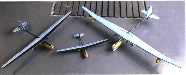
To demonstrate the feasibility of AAM in a physical implementation, the "Flexible Aircraft System Testbed" ("FAST") project was conducted. In this project, three electrically-powered aircraft were manufactured from common tooling to fulfill three different missions, and flight testing was conducted to determine their performance.

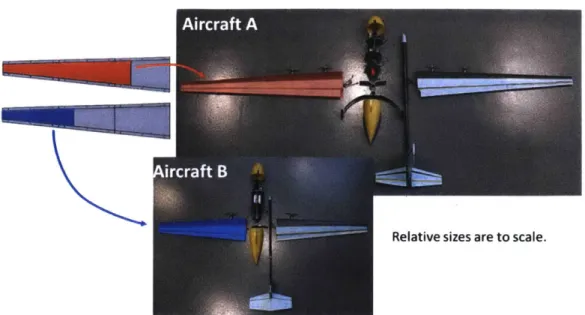
Figure 2.15 shows the three completed aircraft, and Figure 2.16 highlights the wing mold commonality used on the A and B aircraft.

Z

Relative sizes are to scale.

Figure 2.16: Wing commonality between FAST A and B

Aircraft A was designed for a conventional runway takeoff and landing, and was designed for long-endurance loiter. Aircraft B was designed for tool-less assembly to mimic the requirements of small, backpack-deployed military UAS. Aircraft C was designed to carry two spanwise-separated small payloads to fulfill a stereoscopic imaging mission.

One set of molds was used to manufacture the wings, and a second set of molds was used to manufacture both the horizontal and vertical tails (as shown in Figure 2.17). In addition to manufacturing different wing and tail planforms, the layup schedules were altered between aircraft to demonstrate the adjustable-schedule concept, as visible in the differently-colored composite wing construction shown in Figure 2.15.

Figure 2.17. Molds for FAST project (tail: left, wing: right)

In addition to the common wing and tail molding, a spine structure, highlighted Figure 2.18, was used. The fuselage, wing, and landing gear attach to the spine with friction-mounted collars to enable the rapid

mounting and adjustment of aircraft components for testing. While the spine system is feasible for small aircraft, it is not a scalable solution for larger aircraft due to the cube-square law and is therefore not used in the computation investigation performed within this thesis.

Figure 2.18: FAST A (spine in white box)

Table 2.1 below shows the high-level geometric properties of these aircraft, showing a 4.5-fold difference in flight weight and a 3.5-fold difference in wing area between the smallest (B) and largest aircraft (C).

FAST A FAST B FAST C

Wingspan 130 in 72 in 170 in

Length 67 in 44 in 93 in

Wing area 7.7 ft2

3.3 ft2 _{11.67 ft}2

Wing aspect ratio 15.2 10.9 17.2

Flight weight 16.1 lb 5.5 lb 25 lb

Table 2.1: FAST aircraft geometries

Through flight-testing, the following performance estimates are obtained. While these aircraft axe not in any sense optimal, their performance is nonetheless reasonable for small electric vehicles of this class.

FAST A FAST B FAST C

Max endurance 2.6 hours 1.5 hours 1.9 hours

Glide ratio 12.4 11.8 12.2

Climb rate 760 ft/min 700 ft/min 570 ft/min

Stall speed 27 mph 22 mph 28 mph

Dash speed 60 mph 70 mph 50 mph

Table 2.2: FAST aircraft performance

2.3.1 Lessons from FAST and the problem of designing AAM families

While the FAST aircraft proved the viability of creating multiple aircraft from the same set of molds, the experience also highlighted the challenges in performing trade-offs between multiple aircraft:

First, while AAM reduces tooling cost of primary structures, it increases the parts-count and labor in the creation of small, mechanically non-obvious components such as wing joiners, control surface attachment hardware, engine mounts, and mechanisms. For instance, on the FAST project, since the servo locations for each aircraft is different, it was not possible to include the servo pocket into the wing mold, and post-process installations were necessary, increasing both manufacturing time and installed-mass relating to these components.

Second, it becomes extremely difficult to understand what is optimal for the family when variants emphasize different metrics of performance.

Suppose a family were to be designed that includes both an endurance-focused aircraft and a speed-focused aircraft. It is not clear what the optimum tooling, aircraft, nor what the performance penalty would be. In the design of a single aircraft, the optimal design occurs at the resolution of constraints and the pressure gradients of different variables in a design. In the design of an optimal family, the gradients of each variable defining each variant interact with the gradients of the others of the family.

In effect, the question that needs to be answered is, "how expensive are the constraints that AAM places upon these aircraft?" The only way to evaluate such a proposition would be to optimize AAM for the specifics of that particular mission set.

2.4 Way Forward

The remainder of this thesis attempts to address AAM family design by laying out a logical and mathematical structure capable of generating, for any set of mission requirements, the optimal family design. The models must be of sufficient fidelity to capture the inefficiencies generated by the constraints of the architecture. This optimal-family may then be compared against a set of individually-optimal aircraft to determine the performance losses incurred by AAM constraints.

3 ROBUSTNESS AND ADAPTABILITY FRAMEWORK

As discussed in Chapter 1, creating the tooling and production architecture to build an aircraft is much more expensive and time-consuming than creating a single unit. Chapter 2 discussed both the physical implementation of AAM and motivated the necessity of optimizing an AAM family for a given mission set.

The AAM family-design problem may be considered to be an adaptable-robust optimization problem due to the presence of uncertainty (in future missions), a component which is designed and constructed only once (the manufacturing architecture), and an availability of adaptability (in the degrees of freedom within AAM).

The optimization of adaptable-robust systems is complex, and the mathematical organization of this class of problems is an active area of research and debate [13]. Most existing studies in robust optimization use a set of guiding principles and then assemble an ad-hoc structure to solve a particular problem. This chapter presents a framework designed to clarify and organize the interactions in this class of problems, firstly to enable the solution of the AAM performance problem, and secondarily in hopes that such a framework might benefit future robust optimization investigations.

First, to provide a common point of discussion, a classical optimization formulation is presented. Then, uncertainty, robustness, and adaptability are defined qualitatively. These concepts can be difficult to visualize, so an example in the form of an airfoil optimization problem is interleaved with the discussion to illustrate these concepts.

A framework is then presented which captures the dependency and time-rate features inherent in

adaptable-robust problems. This framework shall be used to facilitate the optimization and evaluation of the AAM concept.

3.1 Classical Optimization Formulation

The classical optimization formulation involves the following sets and functions [14]:

x the set of "decision variables" (values to be determined) p the set of "parameters" (values that are imposed a-priori)

g(

)

h(

)

U(

)

The optimization problem may be phrased as:

Find x such that:

min U(x, p)

g (x, p) !; 0 h(x,p) = 0

This formulation is powerful because it can capture a wide range of problems and provides a starting point from which the design problem and solution space may be explored. In the context of aircraft design, aircraft performance requirements are captured within the parameter set p since they are imposed, and are thus not controllable by the designer.

3.1.1 Example of classical optimization: basic airfoil design problem

Suppose the goal of a designer is to design an airfoil for a wing. The designer is given the lift coefficient at which the airfoil must operate, and the goal is to minimize the drag coefficient.

In the context of wing design, the lift coefficient links the weight of the aircraft, the wing area, the air density, and the flight speed. Suppose the thickness of the airfoil is held constant for all designs, and the flow conditions (Reynolds, Mach, etc.) axe identical for all operations. Airfoils change their lift coefficients by changing angle of attack, which is the only degree of freedom available at this stage. First, consider a situation in which flaps are not used.

Nomenclature:

a angle of attack C, lift coefficient

C11 required operating lift coefficient

Cd drag coefficient

s airfoil shape

The optimization problem is phrased as:

Find s, a such that:

min Cd(s, a,C, = C1,1)

Suppose two designs (s, and s2) are being considered; their performance curves are shown in Figure 3.1.

For readers unfamiliar with airfoil performance plotting conventions, the vertical axis (CI) may be considered the independent variable and the horizontal axis (Cd) is the performance metric of interest. In Figure 3.1, the x symbols denote the upper and lower stall limits of each airfoil, so the airfoil may not operate outside of the X-x range.

C,

"General purpose"

.. "Point-design"

Cll1 - ---- -

-CCd

Figure 3.1: Airfoil example: baseline performance

As shown in the figure, the more "point-design" airfoil S2 performs better (lower Cd) at the required C, and would therefore be the preferred design. Also notable is the fact that s2's performance deteriorates faster than si as the C, is changed. This type of local-vs-broad performance tradeoff is typical of many

3.2 Uncertainty, Robust Designs, and Robustness

The term "uncertainty" within this framework refers to a difference between a value used during design and its real value during operation. Uncertainty may arise due to lack of knowledge of operating conditions, naturally-chaotic and unsteady processes, inaccuracy in predictive models, or other sources

[15]. In contrast, "deterministic" problems are defined as those with no uncertainty.

For long-duration projects such as aircraft manufacturing, mission requirements and environment are also uncertain over time - for example, the price of fuel may change due to market forces, the payload mass may change due to the need to install new sensors, or takeoff lengths may change as operators attempt to access new airfields. Uncertainty in mission requirements may be captured by uncertainty distributions in the p-set. This type of uncertainty may be classified as "parametric" (following the classifications defined by [16]).

3.2.1 Robust designs and robustness

A design that is optimal under deterministic assumptions may perform poorly or become infeasible when parameters deviate from their deterministic values. "Robust" designs retain their performance, remain feasible, or a combination of both -despite these variations.

The quantification of robustness is complex and is dependent on the context in which it is explored. Robustness of a design is dependent on the uncertain parameter (in its identity, scope, and distribution) and the metric of performance that the designer selects.

There are two facets of robustness to consider: "sensitivity-robustness" and "feasibility-robustness" which shall be explored in the following example.

3.2.2 Robustness in the airfoil design example

The lift coefficient links lift, air density, speed, and wing area. Some or all of these parameters may vary due to weather, payloads, maneuvers, or other factors, which makes the operating lift coefficient

uncertain. To capture the possible range of C1, new parameters are introduced to the optimization

problem:

C,~ minimum operating lift coefficient C maximum operating lift coefficient

The range of the uncertainty will be called "scope". The optimization problem must now change to reflect the new range of values over which C1 may extend, as shown below:

Find s, a such that:

C+

min

f

For now, it is assumed that the probability distribution between C1_ and C1+ is uniform, so a direct

integration may be used; otherwise, a probability density function would be used to weigh the drag-performance of the airfoil as a function of C1.

First, it is useful to recognize that the scope of the uncertainty affects the choice of the best solution. Figure 3.2 shows a small range of uncertainty, bracketed in orange. Over a small range of C- to C+1, s2 still outperforms s, and remains the superior design.

C,

Ci+

C,

CCd

Figure 3.2: Airfoil example: small uncertain C, scope

However, if the uncertainty scope in C, is large enough, s1 becomes the preferred design, as s, performs

better than s2 over a large range, as shown in Figure 3.3.

CC

C-

_C

Figure 3.3: Airfoil example: large uncertain C scope

This behavior of s, exemplifies higher "sensitivity-robustness" than s2 for this uncertain scope of C since

its performance does not degrade as quickly as C varies away from C11. By comparison, s2 has lower

sensitivity-robustness as its performance degrades faster as C, is changed.

"Feasibility-robustness" addresses the fact that some designs may become infeasible (failing to meet all constraints) given a large-enough perturbation in a given parameter. This category also encapsulates designs in which some minimum amount of performance is required. In this example, if the scope of C is

expanded further, s2 becomes infeasible for some C, within [CC

C].

range where the scope exceeds bounds of the feasible performance space (in red).

C,

--

l

C-/N4

Cd

Figure 3.4: Airfoil example: large uncertain C, range causing infeasibility

In this case, s1 may be considered to have greater feasibility-robustness, as measured by its continued feasibility over a greater scope of C1.

While in this airfoil example, s. has greater sensitivity-robustness and feasibility-robustness, it is important to note that one does not in general imply the other.

3.2.3 Asymmetry in robustness

It is important to note that both sensitivity-robustness and feasibility-robustness of a design may be asymmetric or even discontinuous. Wing structures, for instance, are typically designed up to some "design load" which is separated by a margin to its "ultimate load" beyond which point it shall break. However, the load may be decreased to 0 without failure.

3.3 Passive and Active Robustness and Adaptability

There are multiple ways in which robustness may be achieved. Designs may incorporate "adaptable" features in which one or multiple degrees of freedom exist which allow a designer or user to alter the system in response to variations in an uncertain parameter. This definition is in contrast to "passive" features, which achieve robustness without being adjusted. Complex systems often utilize a combination of both adaptable and passive features.

Under this definition, examples of "fully-passive" systems include most architectural installations such as bridges. Bridges are engineered with sufficient margin above their expected loads, which makes them robust to some amount of overload. However, the bridge is not adjusted in response to the loading scenario.

3.3.1 Adaptable robustness in the airfoil design example

In the above discussion, the airfoil shapes are passively providing robustness since their shapes do not change in response to the change in C1. Suppose now that the designer considers the usage of flaps on