Deterimination [sic] of focal depths of earthquakes in the mid-oceanic ridges from amplitude spectra of surface waves.

by

YI-BEN TSAI

B. S., National Taiwan University (1962)

M. S., National Central University (1965)

SUBMITTED IN PARTIAL FULFILLMENT OF THE REQUIREMENTS FOR THE

DEGREE OF DOCTOR OF PHILOSOPHY

at the

MASSACHUSETTS INSTITUTE OF TECHNOLOGY June, 1969

Signature of Author

Departm t of Earth and Planetary Sciences Certified by

Accepted by

Chairman, Departmental Committee on Graduate Students

IES

ABSTRACT

Deterimination of Focal Depths of Earthquakes in the Mid-Oceanic Ridges from Amplitude

Spectra of Surface Waves

by

Yi-Ben Tsai

Submitted to the Department of Earth and Planetary Sciences in partial fulfillment of the requirement for the

degree of Doctor of Philosophy.

A method based on the normal mode theory for surface waves excited by a slip dislocation in a multilayered clastic medium is successfully developed tor determining the focal depths of remote earthquakes with known fault plane solutions. After examining various possible sources of uncertainty and testing on several earthquakes, the method is si-own to be dependable for studying earthquakes with magnitude mb : 6.

Since the amplitude spectra bf surface waves arc used in this method, not only the focal depth but also the seismic moment of the equivalent double couple system of an earthquake can be determined.

32 earthquakes with known fault plane solutions and in the three major mid-oceanic ridge systems of the world are studied by this method. Our results can be surmmarized as the following:

(1) All strike-slip carthquakes from the east Pacific rise, the Gulf of California, the San Andreas fault, the Mendocino fracture zone, the Blanco fracture zone and the Queen Charlotte Island fault occurred at depths within 10 km excluding the

water depth. This similarity of focal depth distribution

strongly supports Wilson's (1965a,b) ideas that the San Andreas fault is a transform fault, and that the east Pacific rise ex-tends through the tectonic features mentioned and terminatea at the Queen CharloCAtc island fault.

All the strike-slip earthquakes from the mid-Atlantic and tle mid-In dian ocean ridges were also characterized by extremely shallow focal depths.

lithosphere beneath the central ridges is at least 65 km. (3) By using Aki's (1967) scaling law for seismic spec-trum, the observed seismic moments are translated to the sur" face wave magnitude Ms and compared with the body wave magni-tude mb. The results show that all earthquakes, whether dip-slip or strike-dip-slip, follow the same Ms-versus-mb relationship as that observed for earthquakes in the western United States. This similarity of the Ms-versus-mb relationship again supports

the idea that the seismicity in the western United States is closely related to the east Pacific rise. It also implies that the low stress drop observed for earthquakes on the San Andreas fault probably characterizes those earthquakes on the mid-oceanic ridges too.

The surprisingly uniform pattern in focal depth distribution and the unique Ms-versus-mb relationship existing among earth-quakes in all three major mid-oceanic ridges are strong evidence

for the concept of new global tectonics. (Isacks, et. al., 1968).

Thesis Supervisor: Keiiti Aki Title: Professor of Geophysics

I am deeply grateful for the extremely inspiring advice given by Professor Keiiti Aki during the writing of this thesis. In fact, I have learned from him the joy of being a seismologi-cal worker.

I am also indebted to Professor Frank Press. His sugges-tion on using the radiasugges-tion patterns of surface waves to study the transform faults has been influential in defining problems for this thesis.

Very valuable assistance and advice provided by other persons are greatly appreciated, among them are many of my

fellow graduate students.

I owe whatever I may accomplish to my parents, my wife Chu-jen and her parents. My parents have struggled hard to provide me an opportunity for higher learning for which they were denied. My wife's affection and understanding have made this opportunity much more meaningful and fruitful. Her

parents' encouragement is another important source of inspi-ration I have received constantly.

My wife's drafting and Mrs. Shu-Mei Chung's typing have made the appearance of this thesis possible. I thank both of them.

The work of this thesis was supported partly by the Air Force Office of Scientific Research under contract AF49(638)-1632, and partly by the National Science Foundation under Grant GA-4039.

Abstract

Acknowledgments Table of Contents

Chapter 1 - INTRODUCTION

Chapter 2 - EXCITATION OF SURFACE WAVE DUE TO DISLOCATION SOURCES IN A MULTILAYERED MEDIUM

2.1 The Fourier spectra of surface waves due to a point source in a layered half-space

2.2 _{Effects of the crustal thickness under} continents on the excitation of Rayleigh waves

2.3 Effects of the water depth over oceans on the excitation of Rayleigh waves 2.4 Variations of the amplitude spectrum

of surface waves due to a small

uncertainty on the fault-plane solutions 2.5 The effects of finiteness of a source

on the amplitude spectrum of surface waves

2.6 The Fourier spectrum of the source time function

Chapter 3 - EQUALIZATION OF THE OBSERVED AMPLITUDE SPECTRUM OF SURFACE WAVES

3.1 Correction for the instrumental response 3.2 Corrections for the geometrical spreading

and attenuation

3.3 Measurements on the attenuation coeffi-cient of Rayleigh waves by the two-station method

3.4 Tests on the proposed method for focal depth determination

Chapter 4 - THE FOCAL DEPTHS AND THE SEISMIC MOMENTS OF EARTHQUAKES ON THE MID-OCEANIC RIDGES 4.1 Earthquakes on theeast Pacific rise, in

the Gulf of California, western North American and the northeast Pacific region 4.2 Earthquakes on the mid-Atlantic ridge 4.3 Earthquakes on the mid-Indian ocean ridge 4.4 The focal depths of earthquakes on the

mid-oceanic ridges

4.5 Interpretation of the seismic moment data

10 11 26 30 33 40 45 49 50 51 55 64 77 80 102 113 129 131

page Chapter 5

5.1 5.2 5.3

- SUMMARY AND DISCUSSIONS on the method on the results Future studies References 135 135 137 139 140

Recently, seismological evidence (Sykes, 1967) has pro-vided a strong support for the hypotheses of sea-floor spread-ing, transform faults and continental drift. This evidence may be summarized briefly as the following:

Seismic activity on a fracture zone is confined almost exclusively to the section between the displaced ridges. Earthquakes in this zone are characterized by predominantly strike-slip motion. On the other hand, earthquakes located on the ridge crests are characterized by predominantly dip-slip motion. The inferred axes of maximum tension for these dip-slip faults are approximately perpendicular to the local strike of the ridges.

Unfortunately, the evidence mentioned above does not include information on the tectonics of ridges in three space dimensions because of the lack of adequate method to determine the focal depth of remote earthquakes. The purpose of the present paper is to fill in such information by determining the focal depths of e'rthquakes on the mid-oceanic ridges using the amplitude spectra of surface waves.

The focal depths of remote earthquakes such as those from the mid-oceanic ridges can not be accurately determined by travel time data alone. For example, Basham and Ellis (1969) have recently pointed out that the USCGS depths determined on a least-squares basis from P-travel times are, conservatively,

have attempted to use depth phases such as pP or sP for focal depth determination. But this approach has some serious short-comings when it is used for shallow earthquakes. LaCoss (1969) using depth phases at LASA to determine focal depths of nearly

200 events found that sP or pP was correctly picked for only 42 - 57% of all earthquakes. Basham and Ellis (1969) used a

non-linear "P-Detection" polarization filter to isolate

com-pressional and shear phases of 41 seismic events recorded at Western Alberta. They were able to detect the pP phase foz' only 25 of the 41 events. The accuracy of focal depths deter-mined for these 25 earthquakes was about + 15 km. From these two examples we notice that the depth phases were available

for only less than 60% of all earthquakes studied. Furthermore, it is almost impossible to identify these phases for very

shallow earthquakes. Since most earthquakes from the mid-oceanic ridges are remote and presumedly shallow, these classical approaches can not give accurate determination of their focal depths.

The method used in the present paper is based on the normal mode theory for surface waves excited by a slip

dis-location in a realistic, multilayered earth model. This method was first proposed by Yanovskaya (1958). She and several other authors such as Ben-Menahem (1961), Harkrider (1964), Haskell

(1964), Ben-Menahem and Harkrider (1964) and Saito (1967) solved the theoretical problems behind the method. We shall

be applied to surface waves with periods 10 to 50 seconds from earthquakes with known fault plane solutions and with magnitudes smaller than about 6.5.

In the following chapters, several factors affecting the accuracy of the method will be first investigated in de-tails. The applicability of the method will be tested using the data from earthquakes with known depths. We shall then apply this method to determine focal depths of more than thirty earthquakes in the three major mid-oceanic ridge sys-tems of the world. The results will be discussed in the light of the theory of new global tectonics (Isack, et. al., 1968).

CHAPTER 2

Excitation of surface waves due to dislocation sources in a multilayered medium

The Fourier spectrum of surface waves due to a dislo-cation source in a layered half-space may be specified as a

product of the following three factors:

a. the spatial factor which is a complex function

determined by the focal depth, the structure of the layered

medium and the orientation of the equivalent force system of the dislocation source;

b. the temporal factor which is the Fourier transform of the source time function; and

c. the finiteness factor which is derived from the simplified assumption that the rupture propagates along the fault plane with a unform speed over a finite distance.

In order to elucidate how the Fourier spectrum of surface waves may be used to determine the focal depths of earthquakes, each of these factors is examined in the following sections.

2.1 The Fourier spectra of surface waves due to a point source in a layered half-space.

Excitation of Surface waves due to point sources in a layered half-space has been studied by several authors, such as Haskell (1964), Harkrider (1964), Ben-Menahem and Harkrider

(1964) and Saito (1967). These studies were all based upon the normal mode theory of surface waves in multilayered medium due to point force systems. Here we shall follow Saito's results.

The mechanism of earthquakes has been investigated ex-tensively using fault plane solutions based on the first motions of P and polarization of S waves. A large number of

such fault plane solutions now exist. Wickens and Hodgson (1967) give a collection of those from before 1962, and many

more have since been made using the long period WWSSN stations. All reliable solutions obtained so far are consistent with a

double couple source. 'Furthermore, recent theoretical studies by Knopoff and.Gilbert (1960), Maruyama (1963), Haskell (1964)

and Burridge & Knopoff (1964) show that the equivalency of a slip dislocation along a fault to a double couple in the absence of the fault is valid not only in the static elastic field but also in the dynamic elastic field. Thus for the purpose of

calculating the excitation of surface waves due to an earthquake, we shall represent the earthquake source by an equivalent point double couple. The moment of either component couple of the equivalent double couple is defined as seismic moment (Aki,

m(t) varys as a step function in time, i.e.

m(t)=O when t 0

(1) m(t)=M when t & 0

More sophisticated source time functions shall be dis-cussed in a latter section.

Now let us define the coordinate and the fault plane ge-ometry in Figure 1. The fault is assumed to strike in the X direction and to be located at depth h. The dip angle d is measured downward from the positive Y direction. The slip angle S is measured counterclockwise from a horizontal line on the fault plane. r and

4

azimuth from the epicenter to a point P on the free surface.

) is measured counterclockwise from the fault strike.

According to Saito (1967), the Fourier spectrum of dis-placement due to Love waves observed at P can be written as

M, (o) ZC

YZ

L (W. r, #p /h, d, s)=

4WCIf

- fwY (sin d cos s cos _{246 -- sin 2d sin}

s sin 29

)

Cc

(2)

-{-

2d sin s cos

4#

+cos

d

cos s sin

96

where C is the phase velocity and U the group velocity of Love waves at angular frequency W . Ii in equation (2) is defined by0

2

I= f(z) y, (z) dz (3)

yl(z) and y2(z) in equations (2) and (3) are the normal

FIG. 1. Coordinate and fault plane geometry.

dl0

_y,

dz

-- (4)

SYz

0zY

and the boundary conditions

y2

(o)=y

(-

where

f

medium

at depth z.

Similarly, the Fourier spectrum of displacement due to Rayleigh waves observed at P can be written as

Rz(w4,r,&/hds)=

_.42CUZ,

_74'r

.

Y{

3A(Ah*ZA(1)

sin 2d sin s -

sin 2d sin s cos 2

C 2- \(1b)+2A&(h)(A

-sin d cos s sin 2f + sin 2d sin s

__( (26(A

+1

COS

for the vertical component and

-i 7

Rr( W, r, 6 /h, d, s)=Y 3(0) R W , r, /h, d, s)e 2 (7)

for the radial component. C and U in equation (6) are phase velocity and group velocity, respectively, at angular

fre-quency 6O . Il in (6) is defined as

I1= (z) Y1 (z) + y32(z) dz (8)

Y1 (z), Y2(z), Y3(z) and Y4 (z) are the normal mode solutions

~Iy, 1~2t~)]

0

y,

42-zf2/

Yt

dY

o

o

d

Yc

d Y3

44/Z

C

#FF

d-

fA2)

CZ

and the boundary conditions

TY (0)=y4 (0)Y 1(.00o)=y2 (.00)=y 3 '~=Y 4-o =0 (10)

y2

4

1

2

3

4(o)01)

jf(z),

rigidity and the Lame' constant, respectively, of the medium at depth z.

All the normal mode solutions Y's must be continuous at

any depth including the layer interfaces and the depth at

which the source is located. Both the system of equations (4) and (5) and the system of equations (8) and (9) are eigenvalue problems and can be solved either by Haskell's (1953) matrix method or by the Runge-Kutta method of numerical integrations

(Takeuchi et. al. 1964). Once the phase velocity is determined against an angular frequency

w

The group velocity U is then calculated by the following formula (Takeuchi et. al. 1962):

(a) for Love waves

U=I2 c 1 (11)

where I, is defined by equation (3) and 12=

f

12(z) dz (12)

(b) for Rayleigh waves

U=2

+I

)a

+c(I

+I

(13)

20 _CI

1

where I is defined by equation (8) and

I

2=

A(z) Y

(z)

dz

(14)

I3=-2 jAz) Y₃ (z) dz (15)

'5= f (z)[Y (z) +2 Y32 (z dz (16)

I6=2

(z)

Y

(z)

dz

(17)

Once the phase velocity, group velocity and the normal mode solutions Y's at angular frequency w> are obtained for a medium, it is easy to calculate the Fourier spectrum of Love waves by equation (2) and that of Rayleigh waves by equations

(6) and (7) due to a dislocation point source. The source parameters present in these equations are the dip angle d, the slip angle S and the focal depth h. Another source parameter, i.e. the seismic moment M, enters these equations simply as a scalar factor. Thus, either the phase spectrum or the shape of the amplitude spectrum of surface waves can be used to

determine the focal depth h of an earthquake if its fault-plane solution is known. In the present paper, the amplitude spectrum shall be used because in this way we shall be able to obtain simultaneously the seismic moment and the focal depth of an earthquake. The phase spectrum shall be used in the future to study the regional variations of the phase velocity of surface waves.

In calculating the theoretical surface wave amplitude spectrum, we shall choose the frequently used Gutenberg model

(Dorman, et. al. 1960) for the continental paths and the Harkrider-Anderson model (1966) for the oceanic paths.

The layer parameters of the Gutenberg model are given in Table 1. The crust of this model consists of two layers with an equal thickness of 19 km.

The layer parameters of the Harkrider-Anderson model are given in Table 2. The uppermost portion of this model consists of a 5-km water layer, an 1-km sedimentary layer and an oceanic crustal layer of 5km. As compared with the Gutenberg continental model, the Harkrider and Anderson oceanic model has a shallower

and more pronounced low-velocity zone in addition to a thinner crustal wave guide.

Each layer in Table 1 and Table 2 is assumed to be homogeneous. The effects of the crustal thickness in the continental

model and the effects of the water depth in the oceanic model upon the amplitude spectrum of surface waves shall be discussed

TABLE 1. Layer Parameters of the Gutenberg Model Used in This Paper.

Depth(km) f(g/cm3) c((km/sec) j3(km/sec)

0-19 2.74 6.14 3.55 19-38 3.00 6.58 3.80 38-50 3.32 8.20 4.65 50-60 3.34 8.17 4.62 60-70 3.35 8.14 4.57 70-80 3.36 8.10 4.51 80-90 3.37 8.07 4.46 90-100 3.38 8.02 4.41 100-125 3.39 7.93 4.37 125-150 3.41 7.85 4.35 150-175 3.43 7.89 4.36 175-200 3.46 7.98 4.38 200-225 3.48 8.10 4.42 225-250 3.50 8.21 4.46 250-300 3.53 8.38 4.54 300-350 3.58 8.62 4.68 350-400 3.62 8.87 4.85 400-450 3.69 9.15 5.04 450-500 3.82 9.45 5.21 500-600 4.01 9.88 5.45 600-700 4.21 10.30 5.76 700-800 4.40 10.71 6.03 800-900 4.56 11.10 6.23 900-1000 4.63 11.35 6.32

TABLE 2. Layer Parameters of the Oceanic Used in This Paper.

Depth(km) f(g/cm3) oC(km/sec) 0-5 1.030 1.520 5-6 2.100 2.100 6-11 3.066 6.410 11-20 3.400 8.110 20-25 3.400 8.120 25-40 3.400 8.120 40-60 3,370 8.010 60-80 3.370 7.950 80-100 3.370 7.710 100-120 3.330 7.680 120-140 3.330 7.777 140-160 3.330 7.850 160-180 3.330 8.100 180-200 3.330 8.120 200-220 3.330 8.120 220-240 3.330 8.120 240-260 3.330 8.120 260-280 3.350 8.120 280-230 3.360 8.120 300-320 3.370 8.120 320-340 3.380 8.120 340-360 3.390 8.240 360-370 3.440 8.300 370-390 3.500 8.360 Model

A

(km/sec)

Depth(km) 390-415 415-435 435-445 445-465 465-490 490-515 515-540 540-565 565-590 590-615 615-640 640-665 665-690 690-715 715-740 740-765 765-790 790-815 815-840 840-865 865-890 890-915 915-940 940-965 965-990 TABLE 2.-Continued J'(g/cm3) o,(km/sec) 3.684 8.750 3.880 9.150 3.900 9.430 3.920 9.760 3.933 9.765 3.948 9.775 3.960 9.780 3.988 9.784 4.022 9.788 4.056 9.792 4.090 9.796 4.120 9.800 4.165 10.163 4.212 10.488 4.257 10.818 4.300 11.120 4.475 11.135 4.633 11.150 4.797 11.165 4.940 11.180 4.943 11.224 4.945 11.267 4.948 11.310 4.950 11.350 4.952 11.392

A(km/sec)

Several examples are given here to illustrate how the

amplitude spectrum of surface waves varys with the focal depth. Figure 2 shows the Rayleigh wave amplitude spectrum between periods 10 and 50 seconds from a vertical strike-slip fault (d=900, s=00) buried at various depth h within the Gutenberg

model. Figure 3 shows the corresponding Love wave amplitude spectrum. The seismic moment is assumed to be a unit step function in time, i.e. M=l dyne-cm in equation (1). The

observation point is at the azimuth of 300 from the strike and 2000 km away from the epicenter. The number accompanying each curve in the figures indicates the focal depth in kilometers.

Figure 2 suggests that the Rayleigh wave amplitude spectrum in periods 10 to 50 seconds depends very strongly on the focal depth of an earthquake. This is particularly evident for focal

depth less than 100 km. The spectral node on each curve is

caused by the sign reversal of Y3 in equation (6). Thus, the Rayleigh wave amplitude spectrum in this frequency range may be used to determine the focal depths of shallow earthquakes.

Fortunately, the prospect of such an approach is strengthened by the fact that surface waves from shallow earthquakes of medium magnitudes are most clearly recorded in this frequency

range by the WWSSN long period seismographs.

Excitation of Love waves in the continental model also varys with the focal depth as shown in Figure 3. However, the

dependence is weak for focal depth less than 20 km because the normal mode solutions y's decay very slowly with depth in this

Rz

(CONTINENTAL)-P (2000,30)

20 30

PER IOD (SEC)

40 50

FIG. 2. Amplitude spectrum of Rayleigh waves from a vertical strike-slip fault in the

Gutenberg continental earth model.

--10-2 6

-27

- 55.0

not effectively be used to determine the focal depth of a very

shallow earthquake.

Figure 4 shows the Love wave amplitude spectrum at the ocean floor excited by a vertical strike-slip fault buried in the oceanic model at various depth measured from the ocean floor. Figure 5 shows the corresponding Rayleigh wave amplitude spec-trum. As shown in Figure 5, the Rayleigh wave amplitude spec-trum again depends strongly on the focal depth of an earthquake located at depth less than 100 km. On the contrary, Figure 4

shows that the Love wave amplitude spectrum varys very little with the focal depth when the earthquake is less than 100 km

deep. The effect of focal depth in this case would appear in periods shorter than 10 seconds which are outside our frequency range.

In the present paper we are interested in determining the focal depths of many strike-slip earthquakes occurred on the fracture zones and presumed to be shallow. We shall use

primarily the Rayleigh wave amplitude data. Love waves shall be used only as a supplement when required. Another disadvan-tage we may have in using Love wave data results from the fact that Love waves suffer greater scattering due to lateral in-homogeneities in the crust and the upper mantle.

It should be mentioned that the strong dependence of Rayleigh wave amplitude spectrum an the focal depth exists not only for a vertical strike-slip fault as shown in the examples but also for other types of fault as will be shown

I

I

I

|

I

=90*

PER rOD( SEC)

FIG. 3. Amplitude spectrum of Love waves from a vertical strike-slip fault in the Gutenberg continental earth model.

0.0 L(OCEANIC) 1Q5 P (20 00,30) d=90* s=0* io-26 27.5 105.0; 65.0

~

I

I

I

I

I

FIG. 4. Amplitude spectrum of Love waves from a

vertical strike-slip fault in the Harkrider-Anderson oceanic earth model.

..

I

FIG. 5. Amplitude spectrum of Rayleigh waves from a vertical strike-slip fault in the

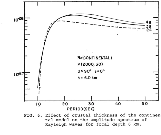
2.2 Effects of the crustal thickness under continents on the excitation of Rayleigh waves

It is well known that the crustal thickness under continents varys from one place to another. We shall now examine how the excitation of Rayleigh waves is affected by changing the crustal

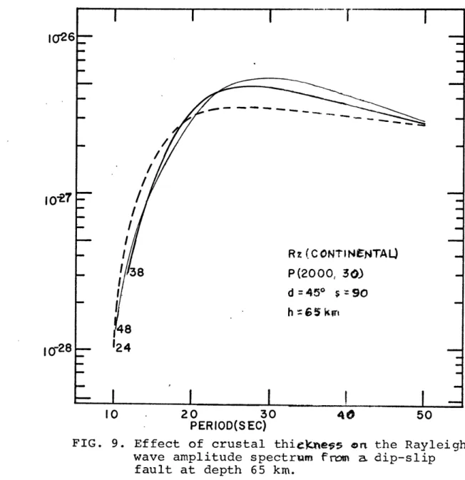
thickness of the Gutenberg continental model. We have calcu-lated the amplitude spectrum of Rayleigh waves for two con-tinental models with a crust of 24 km in one and 48 km in another. The Rayleigh wave amplitude spectrum from a strike slip fault is shown in Figure 6 for a focal depth of 6km and in Figure 7 for a focal depth of 65 km. The number attached to each curve in the figures corresponds to the crustal thickness

in km. Figure 6 and Figure 7 suggest that the effect of the crustal thickness on the Rayleigh wave amplitude spectrum is minor no matter whether the fault is within or below the crust. The same remark can also be made about a pure dip-slip fault dipping at 45 , as shown in Figure 8 and Figure 9. Therefore we shall use the Gutenberg model with a crust of 38 km for all continental paths without regard to possible variations of the crustal thickness over individual paths.

20 30 PE R IOD(S E C)

40 50

FIG. 6. Effect of crustal thickness of the continen-tal model on the amplitude spectrum of

Rayleigh waves for focal depth 6 km.

FIG. 7. Effect of crustal thickness on the Rayleigh wave amplitude spectrum for focal depth 65 km.

- .~ ~. -~

-7

-I

I

I

I

I

I

=

I

I

I

I

PER IOD (SEC)

48 Rz(CONTINENTAL) P (2000, 30) d=90* s=0* h = 6.0 km

VI

|

C-26

I

48 Rz(CONTINENTAL) P(20OOO 30) d=450 s=9 0*0 h= 6.0 km

I

I

FIG. 8. Effect of crustal thickness on the Rayleigh wave amplitude spectrum from a dip-slip

fault at depth 6 km. 24 38 48 I (y26

i0-

I026 E-- / - I - I 10-28-Rz (CONTINENTAL) P(2000, 30) d=450 s=90 h =G5kin 124 20 30 PERIOD(SEC) 40

FIG. 9. Effect of crustal thiecness orn the Rayleigh wave amplitude spectrum from a dip-slip fault at depth 65 km.

Io-P

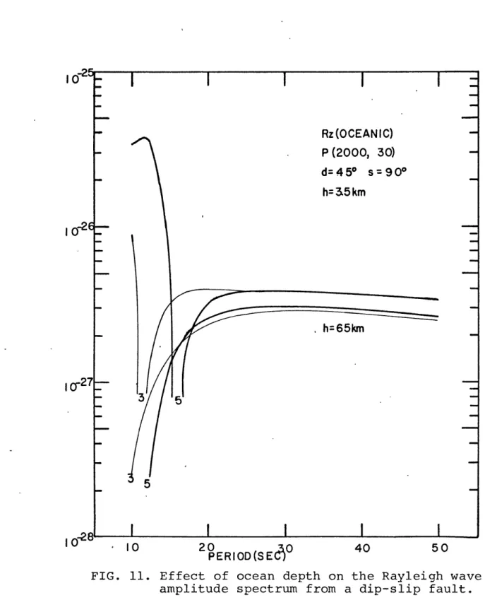
2.3 Effects of the water depth over oceans on the excitation of Rayleigh waves

In the oceanic model given in Table 2, the water depth is assumed to be 5 km. Since different oceanic paths may have different water depth, it is necessary to examine how the ex-citation of Rayleigh waves varys with the water depth. For this purpose, let us reduce the water depth from 5 km to 3 km

in the oceanic model and recalculate the normal mode solutions. The Rayleigh wave amplitude spectrum from a vertical strike-slip fault calculated for this modified model and that calcu-lated for the original model are compared in Figure 10. The same comparison is shown in Figure 11 for a pure dip-slip

0

-fault dipping at 45 . Two focal depths are assumed - 3.5 km

for one and 65.0 km for another. In both figures the heavy curves belong to the original model with 5 km water and the light curves to the modified one with 3 km water. Figure 10 and Figure 11 indicate that the Rayleigh wave amplitude spec-trum appears to be shifted toward shorter periods by a small amount when the water depth is reduced. Fortunately, the shape of the spectrum remains almost unchanged. This would allow us to use the standard oceanic model to interpret the Rayleigh wave amplitude data over oceanic paths by properly adjusting the theoretical amplitude spectrum along the fre-quency axis to accomodate with the known water depth.

I

I

I

=

I

I

I

I

FIG. lo. Effect of'ocean depth on the Rayleigh

wave amplitude spectrum from a strike-slip fault.

I Q -1" h=65km

10'

FIG. 11. Effect of ocean depth on the Rayleigh wave amplitude spectrum from a dip-slip fault.

2.4 Variations of the amplitude spectrum of surface waves due to a small uncertainty on the fault-plane solutions

Sykes (1967) made a comparison of focal mechanism solu-tions for seven earthquakes on the mid-ocean ridges obtained by Stauder and Bollinger (1964a, bj 1965), Stefansson (1966)

with those obtained by himself. He found that with the exception of an event preceded by a small forerunner, the strikes and

dips of the remaining solutions agree within about 150, and within less than 50 for some of the best solutions. For a great many other fault-plane solutions based on data obtained

at modern long-period seismograph networks such as the WWBSN or the Canadian network, the uncertainty on the strikes and the dips may be comparable to that of these six solutions, i.e. within about 150.

The variations of the excitation of surface waves due to

150 of uncertainty on the fault-plane solutions are examined here for two cases: a vertical strike-slip fault and a pure

dip-slip fault dipping at 450* In both cases, either the dip

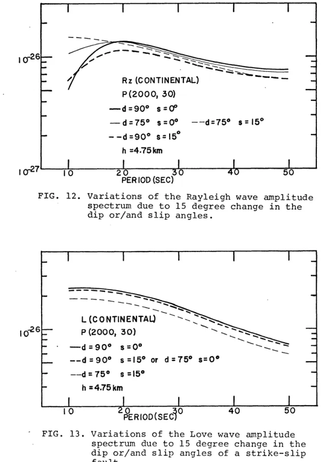
angle or the slip angle or both is varied by 150 * We shall consider each case separately at two focal depths in the Gutenberg model. The amplitude spectral variations due to a

change of 150 in dip or/and slip of a vertical strike-slip fault at 4.75 km are shown in Figure 12 for Rayleigh waves and in Figure 13 for Love waves. The corresponding spectral

variations at focal depth 65 km are shown in Figure 14 for Rayleigh waves and in Figure 15 for Love waves.. As suggested

I

Ole

Irro

I0

I r2

I

I

I

I

PER IOD (SEC)

FIG. 12. Variations of the Rayleigh wave amplitude spectrum due to 15 degree change in the dip or/and slip angles.

-

I

I

I

I

I

=90

=

=15

=4.75km

I

I

I

I

I

FIG. 13. Variations of the Love wave amplitude spectrum due to 15 degree change in the dip or/and slip angles of a strike-slip

Rz (CONTINENTAL) P(2OOO, 30) -- d=75* s=15* I -d=75* s=0'*-II -/ -- d=900 _s=150 -- d=90* s=00 /i h=65km 10 20 30 40 50 PERIOD (SEC)

FIG. 14. Variations of the Rayleigh wave amplitude spectrum due to 15 degree change in the dip or/and slip angles of a strike-slip fault at depth 65 km. - L(CONTINENTAL) P(2000, 30) -d;90* s=0* -d=70* s=0* or d 9Q0 _s=15 0 -- d=750 _s=150 h

=65km

II

I

I

I

FIG. 15. Variations of the Love wave amplitude spectrum due to 15 degree change in the dip or/slip angles of a strike-slip fault at depth 65 km.

by Figure 13 and Figure 15, the variations of Love waves for both source depths are purely scalar and thus cause no change on the spectral shape. Figure 12 and Figure 14 suggest that the Rayleigh wave spectral node is obscured when either the dip or the slip or both of the vertical strike-slip fault are

slightly varied, regardless of its focal depth. This does not, however, mean that the dependence of Rayleigh wave spectrum on focal depth is obscured. On the contrary, the difference between the spectrum from a very shallow earthquake (say at 4.75 km)

and that from a deeper earthquake (say at 65 km) is sharpened. This is due to the fact that the spectral node is located in the short-period end when the focal depth is small and moves toward the long-period end when the focal depth is increased. The obscuring of this spectral node will.then enhance the spectral components on the short-period end when the fault is close to the surface but will enhance those on the long-period end when the fault is at 50 km or deeper.

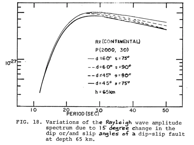
For the case of a dip-slip fault, the spectral variations of Rayleigh and Love waves are shown in Figure 16 and Figure 17 when the fault is at depth 4.75 km and in Figure 18 and Figure 19 when the fault is at depth 65 km. From Figure 17 and Figure 19, we again find that Love wave spectrum is affected only by a small scalar factor if the dip or/and the slip of the dip-slip fault at both depths is altered by 15.0 For a fault very close to the surface, the Rayleigh wave spectrum is

20 3 PERIOD(SEC)

0 40 50

FIG. 16. Variations of the Rayleigh wave amplitude spectrum due to 15 degree change in the dip or/and slip angles of a dip-slip fault at depth 4.75 km.

L (CON TINEN TAL) P(2000, 30) h =4.75km -d

=45*

=

=75

Ii

I

I

I

Variations of the Love wave amplitude

spectrum due to 15 degree change in the dip or/and slip angles of a dip-slip fault at depth 4.75 km. Rz (CONTINENTAL) - P(2000, 30) h 4.75km -d=45* s=90--d=60* s=90* -- d= 45* s=75* -- d=60* s=75*

I

20 30

PERIOD (SEc

FIG. 18. Variations of the Rayle I3h wave amplitude

spectrum due to 16~ degree change in the dip or/and slip

angles

I

I

I

I

I

L .

'10

FIG. 19. Variations of the Love wave. amplitude

spectrum due to chag in

Aip

I

I

I

spectral node is obscured but also the amplitude level is significantly changed. The end effect tends to strengthen the short-period components and weaken the long-period com-ponents. On the other hand, Rayleigh waves are affected very

little when the fault is at 50 km or deeper. Thus we can conclude this discussion by saying that an uncertainty of about 150 of the dip or the slip or both of a fault-plane solution will not seriously affect the accuracy of our method of depth determination.

2.5 The effects of finiteness of a source on the amplitude spectrum of surface waves

The dependence of amplitude spectrum of seismic waves on source size has been derived semi-empirically by Aki (1967) under the assumption that large and small earthquakes are

similar phenomena. This assumption of similarity implies a constant stress drop independent of source size. His results indicate that the W -square model gives a satisfactory ex-planation of observed data. According to this model, the

shape of the amplitude spectrum of displacement for periods longer than 10 seconds is almost independent of earthquake-magnitude for Ms 4 5.5 where Ms is the earthquake-magnitude defined for

surface waves with period of 20 seconds. Even for Ms=6.5 the amplitude at period 10 seconds will be reduced by only a factor of about 2. Since all except four of the earthquakes studied

in this paper have magnitudes mb < 6, the effect of source size on the shape of surface wave amplitude spectrum may be neglect-ed for most of these earthquakes.

The finiteness effect of a source can also be estimated if the length and the rupture velocity of the fault are known. Ben-Menahem (1961) showed that the contribution to the Fourier spectrum of surface waves from a unilateral fault with length L and ruptdre velocity V may be written as

L

Xf i (t -

r -xcos

[ nX

eiX

-+](8

Ix/'

where X=

s j

r is the epicentral distance

2

V

and f the azimuth to a station. C is the phase velocity of the wave.

In order to make a realistic estimation of the amplitude of finiteness factor given in equation (18) some knowledge

about the fault length L and the rupture velocity V is required. A number of shallow earthquakes in various parts of the

world have been found to be associated with surface traces of rupture near their epicenters. Several authors have found approximate correlations between the magnitudes (M) of these shocks and the length of the surface traces of rupture. The first empirical relationship of this type was derived by Tocher

(1958) for ten California and Nevada shocks. lida (1959, 1965)

has studied about 60 shocks occurring world-wide, using in large part data supplied by Richter (1958) and including those of Tocher. Iida obtained results similar to those obtained by

Tocher. Press (1967) found Tocher's curve, although valid for large earthquakes, to be unsatisfactory for shocks of small magnitudes. Press used data of small earthquakes and nuclear explosions to derive a modified relationship between fault

curve, an event of magnitude 4 will have a linear dimension between 0.1 and 1 km. A seismic source with magnitude 5 has a linear dimension between 0.5 and 5 km. King and Knopoff

(1968) added forty-two more shocks with magnitude ranging from

3.6 to 8.5 to this kind of studies. All the results obtained

so far are summarized in Figure 20 which is taken from the paper by King and Knopoff (1968) with no data points included. Their data show that the Imperial shock of 1966 was undoubtedly a

very exceptional case. As for the Parkfield main shock of 1966, if the surface wave magnitude of 6.4 (Wp, 1968), instead 5.5 is used, the deviation from the curve of Press (1967) would be significantly reduced. Thus, for the moment, we shall follow Press' curve and calculate the amplitude of the transfer function in equation (18) by taking L=10 km for an earthquake of magnitude M=6.0 which is the upper limit for most of the earthquakes

studied in this paper (Table 3 to Table 5)

As for the rupture velocity, it varys between 3 and 4 km/sec as derived from detailed studies of several major shallow earth-quakes by the methods of phase equalization, radiation pattern, and directivity (Ben-Menahem, 1967). An average rupture velocity of 2.2 km/sec has been determined by Eaton (1967) for the

Parkfield, 1966 earthquake using the data obtained at the Gold Hill station which was in the fault zone 20 km southeast of the epicenter. This is believed to be the only rupture speed

obtained so far by a method not associated with surface wave or free oscillation data. In order to make an estimate of

maximum effect due to the finiteness of sources, we shall choose the smaller rupture velocity, i.e. 2.2 km/sec in our calculations.

Figure 21 gives the factor of

for Rayleigh

waves in the Gutenberg continental model. Two azimuths

(9$

450 and 1350 ) corresponding to the lobe directions of a

vertical strike-slip fault are considered. From this figure, we find that the effect of finiteness is negligible on the forward quadrants of the propagating fault. Even on the back-ward quadrants, the effect is limited to periods less than 20 seconds or so. This is believed to be a maximum estimate of finiteness effect because the rupture velocity used bare is on the lower end of most observed values and the length of fault on the longest end. A greater rupture velocity, say 3 km/sec, would reduce this effect significantly. Based on

this evidence the finiteness factor shall be neglected in our interpretation of those events whose fault length and rupture

log L (L in cm)

FIG. 2o. Earthquake magnitude versus fault length.

20 30

PERIOD(SEC)

FIG. 21. Effect of finiteness on the Rayleigh wave amplitude spectrum. 1.0 0.5 0.1

I

|

|

|I

-- $=45*

2.6 The Fourier spectrum of the source time function

In all calculations we have made so far, a unit step

source time function defined by equation (1) (with M=l'dyne cm) is assumed. Although this function has been found to be con-sistent with most observed surface wave data from shallow earthquakes (Ben-Menahem, 1967), other functions have been

proposed to represent the source behasrior in time. Among these

are a ramp function and a function varying as

m(t)=0 when t

<

m(t)

=M(1-e-t/

As shown in Figure 22a, these two functions are comparable to each other. Thus we shall consider here only the latter one.

The Fourier spectrum of the function defined by equation

(20) can be written as

W W)= , M ' (21)

This spectrum differs that of a step function defined in

equation (1)

only by a simple factor

(

)

.

The

significant over the whole period range from 10 to 50 seconds. Ben-Menahem and Toks6z (1963) used the observed phase spec-trum of the source time function to obtain a 2 =22 seconds for the Kamchatka earthquake of November 4, 1952 which had a magnitude of 84 and a fault length of 700 + 50 km. Hirasawa

m(t)

m(t)=M (-e~I )

FIG. 22a. A source time function.

20 30

PERIOD(S EC) 40 50

FIG. 22b. The Fourier amplitude ratio between the source time function shown in FIG. 22a and the step function given by Eq. (1). 1.0 0.5 0.1

I

I

I

~

I0I

June 16, 1964 as 2 to 4 seconds by equalizing the wave energy in a finite frequency range obtained from the observed P wave to that theoretically expected. According to Aki (1966) and Hirasawa (1965), this earthquake was caused by a dip-slip fault with a total length between 80 to 100 km. Haskell

(1969) used a two-stage ramp source time function to explain

the acceleration pulse measured by the strong-motion accel-erometer near the fault of the Parkfield earthquake of June 28, 1966. His results showed that the rise time is about 0.9

second. Aki (in press) used a slightly different technique to obtain 0.4 second for the rise time of the same earthquake. The Parkfield earthquake has a fault length of almost 40 km

and a surface wave magnitude of 6.4. Although there is still no observation on the rise time of smaller earthquakes, it seems reasonable to say that the rise time for an earthquake with magnitude 6.0 or less and with a fault length of about

10 km may be well within one second, Based on this evidence

we may conclude that for most earthquakes studied in the

present paper, the source time function can satisfactorily be represented by a step function as defined in equation (1).

After having considered each factor that contributed to the source spectrum of an earthquake, we feel that the theoreti-cal amplitude spectrum of surface waves theoreti-calculated on the as-sumption that the source is a point in space and a step function in time can be used to interpret data obtained from earthquakes with magnitude 6.0 or smaller without serious errors. For the

uncertainty of 150 or less on the dips or/and the slips of the fault plane solutions for shallow earthquakes seems to be

tolerable.

The foregoing discussions are concerned with the theoretical part of the proposed method. We shall consider now the obser-vational part in next chapter with the aid of several testing cases.

CHAPTER 3

Equalization of the observed amplitude spectrum of surface waves

As a surface wave train spreads out on its way to a recording station, its Fourier spectrum is modified by:

(a) attenuation due to the anelasticity of the earth's crust and upper mantle*

(b) scattering due to the lateral inhomogeneity present

over the propagation path;

(c) dispersion, geometrical spreading and the polar phase shift over a spherical earthy and

(d) the filtering effect of the recording instrument.

The process of removing these distorting effects is known as the amplitude and phase equalization of the surface wave

spectrum.

In the present study the amplitude equalization method (Toksaz, et. al., 1964; Aki, 1966; Tsai and Aki, 1969) shall be used. By applying this method to an earthquake with known fault-plane solution its focal depth and seismic moment can

be determined simultaneously.

In the following sections, we shall first describe the method and then use several examples to illustrate its appli-cability and limitations.

3.1 Correction for the instrumental response

In the present paper we shall use the WWSSN long-period seismograms.

Attempts have been made to choose an appropriate procedure of correcting for the instrumental response. The magnification curve calculated from appropriate instrument constants by

Hagiwara's formula (1958) was compared with those obtained from analysing the calibration trace on the corresponding record for many stations.

In general, the agreement between these two were quite close at long periods but not at short periods, probably due to some contamination of the calibration trace by microseismic noises. Thus, we shall make the instrumental correction

through the magnification curve calculated by Hagiwara's formula with a proper choice of the following instrument constants:

Seismometer: To=15 or 30 seconds, 6o

=0.93

magnification 6000 3000 1500 750 375 coupling coefficient 0.805 0.204 0.047 0.013 0.003

3.2 Corrections for the geometrical spreading and

attenuation

After the observed amplitude spectrum of displacement is corrected for the instrumental response by the method

described in previous section, it should further be corrected for the geometrical spreading and attenuation by the following relation:

A(w)0=A(a)){ i"'

rj

(22)

where Ar(O) is the amplitude observed at the station r km

(or 4 _{r degree) from the epicenter; 7% (W) is the attenuation}

coefficient at angular frequency w 7 Ao(w ) is the equalized amplitude at

r

radius in km. We shall choose r1 =2000 km.

The equalized amplitude Ao(4o) corresponds to the displa-cement spectral density observed at

r

The correction for attenuation enters equation (22)

through the attenuation coefficient (W'). Data on 7(6) of Love waves are almost non-existing for periods between 10 and

50 seconds (Sato, 1967).

As for Rayleigh waves, there have been some measurements of T( O) in the past. Arkhangel'skaya and Fedorov (1961)

measured ?I (W ) between 22-24 sec using Rl to R5 observed at

for periods less than 30 seconds reported by various authors. Press (1964) measured QR=3₂5

at period 12 seconds from LRSM records of Nevada nuclear explosions. A more systematic meas-urement of ( W) was made by Tryggavason (1965). He used the WWSSN records of a nuclear explosion near Novaya Zemlya

in his study. -Tsai and Aki (1969) made a measurement of g (0)

over periods between 15 and 50 seconds from the WWSSN records of the Parkfield, California earthquake of June 28, 1966. Data from all these measurements are summarized in Figure 23. The curve on the figure is Tryggavason's (1965) would-wide average value. Even with the added data, his curve is still valid. These results seem to suggest that the attenuation coefficient (0) (not Q) of Rayleigh waves can be approxi-mated by a constant over period range from 50 seconds down to

about 15 seconds for the present purpose. For periods shorter than 15 seconds, there is indication of increasing attenuation toward short periods. However, the large variability of the data for the short periods would make any further intepretations less meaningful.

It should be pointed out here that all the data mentioned above have been obtained on a world-wide basis and may not be suitable for use in the present study because the propagation paths are selectively chosen so that each path lies almost entirely in one type of the crustal structure, that is either

oceanic or continental. Therefore we shall make measurements of Rayleigh wave attenuation over paths which are entirely oceanic or entirely continental. The results are presented

0.04 0.05 0.06 0.08 0.09 0. CYCLES PER SEC

FIG. 23. Summary of the observed attenuation coefficient of Rayleigh waves in periods less than 50 sec.

3.3 Measurements on the attenuation coefficient of Rayleigh waves by the two-station method

The attenuation coefficient 4T (W) over the path between a pair of stations nearly on the same great circle can be calculated by

(_)=_

f____

//(23)

(rEx - Ei ) /) (1') Z. A

where A,( W) and A2( w) are the amplitudes at frequency cw

observed at station 1 and station 2, respectively. The epi-central distance of the first station is designated as

f

(

rz

(

By this method, the source effect can be removed. The

uniformity and the availability of the WWSSN long-period records may eventually prove that the two-station method is capable of providing regional attenuation coefficients of surface waves.

Measurements of (60) have been made for Rayleigh waves over three paths - one oceanic (KIP-BKS) and two continental

C

(BOZ-WES and GSb-BIA). The sources were three earthquakes from the Solomon Islands area:

(a) July 17, 1965, 12:47:48.7 GMT mb=6.4 (b) November 27, 1965, 12:01:51.5 GMT, mb=6.0

(c) January 13, 1967, 13:48:11.7 GMT, mb=6.0

Let us now examine the data from each path more care-fully.

(1) The east Pacific basin between KIP (Honolulu) and BKS (Berkeley) :

The path is oceanic almost all over its entire length of 3880 km except a short portion before reaching BKB where the ocean-continent boundary is crossed. Unfortunately we were able to make only one measurement because the records of the remaining two events were not available at one of the two stations, The observed amplitude spectra at both stations and the corresponding amplitude ratio are shown in Figure 24a and Figure 24b, respectively. In Figure 24a, the epicentral distance and the azimuth-at the source, measured clockwise from due north, of the great-circle path leading to each station are also given in the parenthesis following the station code. From this figure, we can see that the general form of the spectrum has been well maintained along its path from KIP to BKS. The phenomenum is again illustrated by the lack of fre-quency dependence of the amplitude ratio as shown in Figure

24b. The data for periods below 16 seconds or so are much

scattered because of their lower amplitude level. The attenuation coefficient ) (&.) obtained from this measurement has a constant value of 168 x 106 km~1 for periods from 10 to 50 seconds.

This is quite similar to the world-wide average value for periods longer than 15 seconds as shown in Figure 23. As far

as our data are concerned, there appears no systematic increase of attenuation for periods shorter than 15 seconds which was observed by Tryggavason (1965). It is probable that scattering and reflections at crossing boundaries between oceans and

con-tinents were responsible for at least part of the attenuation observed by Tryggavason. Although we have no similar

10

20

30

PER

IOD(SEC)

at KIP and BKS.

40

50

gh wave amplitude spectrum

10

20

30

40

50

PERIOD(SEC)

FIG. 24b. The amplitude ratio between BKS and KIP.

0~

-lto-

II

I

I

Rz

(

1-13- 67)

-

KIP

(5677.0,51.3)

BKS (9558.0

,50.5)

|-II

I

I

1.0

0.5

0.1

measurements over other oceans, the close agreement between

our measurement of the Pacific basin (?(W)=168 x 10-6 km~) and those made by Gutenberg (1935) over the Atlantic (4

=

suggests that (4)=168 x 10-6 km~i may be representive for most ocean basins. Most of our oceanic paths are quite similar to that between KIP and BKS in the sense that shortly before the waves reach the recording stations on land, they all have

to cross the ocean-continent boundary. Thus, the attenuation coefficient (C4U) measured from KIP to BKS appears to be

applicable to them at least for the first approximation.

(2) Southern United States between GSC (South California)

and BIA (Virginia):

This is an exclusively continental path of 3250 km running

across the southern part of the United States from the west to the east coast. We have made three measurements on this path. The observed -litudes an shown in Figure 25a and Figure 25c. The correspoi g amplitude ratios from all three measurements are given in ...gure 25b. Again the spectrum was distorted very little after the waves had propagated from GSC to BIA for more than 3200 km. The amplitude ratios show no systematic dependence on frequency. From these three measurements we have obtained a constant value of 157 x 10-6 km~1 for the attenuation coefficient (W) in the period range between 10

and 50 seconds. Again, this value is similar to the world-wide

Rz (

1-13-67)

-0--B

LA( 13210.0,53.5)

Rz (11-27-65)

--

--

-+-BLA (13298.3,52.8)

-I

I

I

I

20

30

40

50

PERIOD(SEC)

-*

Rz (BLA/GSC)

(

1-13-67)

20

30

40

50

PERIOD (SEC)

FIG. 25b. Rz amplitude ratios between BLA and GSC.

1Al

10-2

1.0

0.I

10~-(3) Northern United States between BOZ (Montana) and WES (Massachusetts):

This is an entirely continental path with a rather uniform crustal structure running from west to east for a distance of

3220 km across northern United States. The observed amplitude

spectra from all three events are shown in Figure 26a and Figure 26c. The corresponding amplitude ratios are shown in Figure 26b. These data indicate that the attenuation of Rayleigh

waves is nearly frequency independent as we have pointed out already. However, it is interesting to find here that the

attenuation coefficient obtained here is only about 52 x 10-6 km~1. This is noticeably lower than most values obtained so far. If this low attenuation is proved to be real, then its geophysical implications may be quite significant. For the moment, we shall not pursue further on this aspect.

In summary, results of all measurements along three

different paths appear to indicate that the attenuation

coef-ficient T (J) is approximately independent of frequency for periods between 10 to 50 seconds. Except one possible low attenuation path, the Rayleigh wave attenuation coefficients

obtained from our measurements do not differ much from the world-wide average value. A constant attenuation coefficient

(I ) implies that the quality factor QR would be almost inversely proportional with period for 50> T10 seconds.

This is essentially consistent with the interpretation of Tsai and Aki (1969) that the high Q lithosphere of about 100 km thickness overlies the low Q asthenosphere.

El

|

1

|

|

~7

10 20 30 40 50

PERIOD (SEC)

FIG. 25c. Rz amplitude spectrum observed at GSC and BLA. Rz(7-17-65) 0BOZ(10662.8, 44.9) 0 WES(13881.8,44-7) 20 30 PERIOD(SEC) 40

FIG. 26c. Rz amplitude spectrum at BOZ

I I Rz (7-17-65) 0 GSC (10037.7, 5 4.4) OBLA (13289.5, 52.8) Ie IO 50 and WES.

FIG. 26a.

10~

Rz amplitude _{spectrum at BOZ and WES.}

10

20

30

40

50

PERIOD(SEC)

* ( 1-13-67)

.:

0

I II

10

20

PERIO

30

40

FIG. 26b. Rz amplitude ratios between WES and BOZ.

Rz

( 1-13-

67)

-e-BOZ(10610.0,44.8)

(3829.0,45.6)

-Rz ( l

-

27- 65)

B

,44.7

I

I

I

5.0

1.0

05

10-2

On the basis of our data given above we may conclude that the attenuation effect on the shape of the Rayleigh wave am-plitude spectrum for periods between 10 to 50 seconds may be neglected along a simple path for as long as 3900 km such as

the one between KIP and BKS. Thus the correction for attenuation will appear in equation (22) simply as a scalar factor. In

other words, it will affect only the seismic moment but not the focal depth determination.