Statistics of the CMB polarised anisotropies : unveiling the primordial universe

(1)

HAL Id: tel-01126907

https://tel.archives-ouvertes.fr/tel-01126907

Submitted on 6 Mar 2015

HAL is a multi-disciplinary open access

archive for the deposit and dissemination of

sci-entific research documents, whether they are

pub-lished or not. The documents may come from

teaching and research institutions in France or

abroad, or from public or private research centers.

L’archive ouverte pluridisciplinaire HAL, est

destinée au dépôt et à la diffusion de documents

scientifiques de niveau recherche, publiés ou non,

émanant des établissements d’enseignement et de

recherche français ou étrangers, des laboratoires

publics ou privés.

Statistics of the CMB polarised anisotropies : unveiling

the primordial universe

Agnès Ferté

To cite this version:

Agnès Ferté. Statistics of the CMB polarised anisotropies : unveiling the primordial universe.

Cosmol-ogy and Extra-Galactic Astrophysics [astro-ph.CO]. Université Paris Sud - Paris XI, 2014. English.

�NNT : 2014PA112223�. �tel-01126907�

(2)

Universit´

e Paris-Sud

´

Ecole doctorale 517 :

particules, noyaux et cosmos

Institut d’Astrophysique Spatiale

Discipline : Physique

Th`

ese de doctorat

Soutenue le 26 septembre 2014 par

Agn`es Fert´e

Statistics of the CMB

Polarised Anisotropies

Unveiling the Primordial Universe

Composition du jury :

Directeur de th`ese : Julien Grain Charg´e de recherche (IAS)

Pr´esident du jury : Ken Ganga Directeur de recherche (APC)

Rapporteurs : Jean-Christophe Hamilton Directeur de recherche (APC) Julien Lesgourgues Charg´e de recherche (CERN)

Examinateurs : Martin Kunz Professeur (ITP)

(3)

Abstract

A deep understanding of the first instants of the Universe would not only complete our description of the cosmic history but also enable an exploration of new fundamental phsyics at energy scales unexplored on Earth laboratories and colliders. The most favoured scenario which describes these first instants is the cosmic inflation, an ephemeral period of accelerated expansion shortly after the big bang. Some hints are in favour of this scenario which is however still waiting for a smoking-gun observational signature. The cosmic microwave background (CMB) B modes would be generated at large angular scales by primordial gravitational waves produced during the cosmic inflation. In this frame, the primordial CMB B-modes are the aim of various ongoing or being-deployed experiments, as well as being-planned satellite mission. However, unavoidable instrumental and astrophysical features makes its detection difficult. More specifically, a partial sky coverage of the CMB polarisation (inherent to any CMB measurements) leads to the E-to-B leakage, a major issue on the estimation of the CMB B modes power spectrum. This e↵ect can prevent from a detection of the primordial B modes even if the polarisation maps are perfectly cleaned, since the (much more intense) leaked E-modes mask the B-modes. Various methods have been proposed in the literature o↵ering a B modes estimation theoretically free from any leakage. However, when applied to real data, they are no longer completely leakage-free and remove part of the information on B-modes. These methods consequently need to be validate in the frame of real data analysis. In this purpose, I have worked on the implementation and numerical developments of three typical pseudospectrum methods. Afterwards, I have tested each of them in the case of two fiducial experimental set ups, typical of current balloon-borne or ground based experiments and of potential satellite mission. I have therefore stated on the efficiency and necessity of one of them: the so-called pure method. I have also shown that the case of nearly full sky coverage is not trivial because of the intricate shape of the contours of the point-sources and galactic mask. As a result this method is also required for an optimal B modes pseudospectrum estimation in the context of a satellite mission.

With this powerful method, I performed realistic forecasts on the constraints that a CMB polar-isation detection could set on the physics of the primordial universe. First of all, I have studied the detectability of the tensor-to-scalar ratio r, amounting the amplitude of primordial gravity waves and directly related to the energy scale of inflation, in the case of current suborbital ex-periments, a potential array of telescopes and a potential satellite mission. I have shown that a satellite-like experiment dedicated to the CMB polarisation detection will enable us to measure a tensor-to-scalar ratio of about 0.001, thus allowing for distinguishing between large and small field models of inflation. Moreover, in extension of the standard model of cosmology, the CMB EB and T B correlations can be generated. In particular, I have forecast the constraints that one could set on a parity violation in the gravitational waves during the primordial universe from observations on a small and a large part of the sky. Our results have shown that a satellite-like experiment is mandatory to set constraints on a range of parity violation models. I finally address the problematic of the detectability of observational signature of a primordial magnetic field.

(4)

iii

R´esum´e

La compréhension des premiers instants de notre Univers complèterait notre description de son histoire et permettrait également une exploration de la physique fondamentale à des échelles d’énergie jusque là inatteignables. L’inflation cosmique est le scénario privilégié pour décrire ces premiers instants car il s’intègre très bien dans le modèle standard de la cosmologie. Selon ce scénario l’Univers aurait connu une courte période d’expansion accélérée peu après le Big Bang. Quelques indices favorisent ce modèle cependant toujours en attente d’une signature observation-nelle décisive. Les modes B du fond di↵us comologique (FDC) aux grandes échelles angulaires sont générés par les ondes gravitationnelles primordiales, produites durant l’inflation cosmique. Dans ce cadre, la détection des modes B primordiaux est le but de nombreuses expériences, actuelles ou à venir. Cependant, des e↵ets astrophysiques et instrumentaux rendent sa détection difficile. Plus précisément, une couverture incomplète de la polarisation du FDC (inhérente à toute observation du FDC) entraine la fuite des modes E dans B, un problème majeur dans l’estimation des modes B. Cet e↵et peut empêcher une détection des modes B même à partir de cartes parfaitement nettoyées, car les modes E fuyant (beaucoup plus intenses) masquent les modes B. Diverses méthodes o↵rant une estimation de modes B théoriquement non a↵ectés par cette fuite, ont été récemment proposées dans la littérature. Cependant, lorsqu’elles sont ap-pliquées à des expériences réalistes, elles ne corrigent plus exactement cette fuite. Ces méthodes doivent donc être validées dans le cadre d’expériences réalistes. Dans ce but, j’ai travaillé sur l’implémentation et le développement numérique de trois méthodes typiques de pseudospectres. Ensuite, je les ai testé dans le cas de deux expériences fiducielles, typiques d’une expérience sub-orbitale et d’une potentielle mission satellite. J’ai alors montré l’efficacité et la nécessité d’une méthode en particulier: la méthode dite pure. J’ai également montré que le cas d’une couverture quasi complète du ciel n’est pas trivial, à cause des contours compliqués du masque galactique et des points sources. Par conséquent, une estimation optimale de pseudospectre des modes B exige l’utilisation d’une telle méthode également dans le contexte d’une mission satellite. Grâce à cette méthode, j’ai fait des prévisions réalistes sur les contraintes qu’une détection de la polarisation du FDC pourra apporter sur la physique de l’Univers primordial. J’ai tout d’abord étudié la détectabilité du rapport tenseur-sur-scalaire r qui quantifie l’amplitude des ondes gravitationnelles primordiales, directement relié à l’échelle d’énergie de l’inflation, dans le cas de di↵érentes expériences dédiées à la détection de la polarisation du FDC. J’ai montré qu’une mission satellite nous permettrait de mesurer un rapport tenseur-sur-scalaire de l’ordre de 0.001, autorisant une distinction entre les modèles d’inflation à champ fort et faible. De plus, dans le cas d’une extension du modèle standard de la cosmologie, des corrélations EB et T B du FDC peuvent être générées. En particulier, j’ai prévu les contraintes que nous pourrons mettre sur une violation de parité durant l’univers primordial à partir d’observations sur une grande ou une petite partie du ciel. Mes résultats ont montré qu’une expérience satellite est nécessaire pour mettre des contraintes sur une gamme de modèles de violation de parité. J’ai finalement abordé la problématique de la détectabilité d’une signature observationnelle d’un champ magnétique primordial.

(5)

Acknowledgements

Elle est un peu difficile à écrire cette partie. D’abord car c’est important pour moi de remercier les personnes qui ont compté, ensuite parce qu’il parait qu’on ne lit généralement que cette partie, ¸ca fout la pression. Mais bon, je suis encore à la bourre pour rendre le manuscrit alors voilà :

Tout d’abord, nonante mercis à Jean-Christophe Hamilton et Julien Lesgourgues d’avoir ac-cepter de lire, commenter, questionner et reporter ce manuscrit. Merci beaucoup aussi à Ken Ganga, Martin Kunz et Jean-Loup Puget (bien qu’absent) pour vos commentaires et questions intéressantes. Merci à vous d’être sympathiques et de bonne humeur, rendant la soutenance légèrement moins stressante.

Travailler avec des personnes scientifiquement excellentes m’a énormément stimulé, merci à Julien Peloton (je te souhaite une pure fin de thèse!), Radek Stompor (entre autres pour avoir pointé des choses à étudier qui ont doublé mon temps de travail sur le sujet) et Matthieu Tristram. Ca fait quelques temps que je trainasse à Orsay. Merci à mes profs motivants et aux encadrants de mes premiers stages de recherche. Merci à Hervé pour (G)ALCOR, de m’avoir dit ’tiens, tu devrais aller avoir Julien Grain & co à l’IAS, ils ont peut être une proposition de thèse’ un jour de mars 2011, et pour ton entrain. D`ıky moc à Mathieu, son bureau (lieu de craquage, s’il en est) et JB pour les geek nights, les mots fléchés, votre curiosité et vision di↵érente. Orsay, c’est le magistère et NPAC où j’ai rencontré des personnes sans qui les études et la thèse auraient été di↵érentes (et moins bien pour sûr): tellement merci à Gé2 _{et ses pestougnèses} défiant la gravité, Schmi et son petit macaquon (bon courage à vous pour la fin de thèse!), et puis Matthieu, Benjamin, Pierre, (I am not a...) Tico, Guillaume, Julian, Flavien qui ont trop participé à l’élévation de mon alcoolémie, et enfin Vincent, Guigui, Asénath, Estelle, Samuel Franco, Jérémy, Marie, Marco mon binome, ses pastas et les repas NPAC. On s’est bien marré quand même, bon vent pour vos chemins respectifs.

Je suis contente d’avoir fait mes débuts en recherche à l’Insitut d’Astrophysique Spatiale, un laboratoire à la fois travailleur et vivant. Enorme merci à tout le laboratoire, du person-nel administratif jusqu’aux doctorants, pour tout dont les petit mots, votre générosité et cette soirée. Merci à l’équipe MIC et en particulier au groupe cosmologie dont Nabila et Marian, pour vos explications, votre curiosité et garder votre sympathie malgré la pression. Héxa merci à

Véronique, Sébitouf & Heddy (heureusement que vous êtes partis sinon j’aurais fait une thèse en QPUC/TLMVPSP/blagues salaces (d’ailleurs...)), 2Fab, Aurélie, cobureau Cédricounet, Guil-laume H. pour les pauses scientifiques (et les stupides aussi), Antoine, c’était cool d’être ta suppléante: merci pour ta volonté de changer les choses (j’aime), et puis à tous les thésard-es et post-docs d’hier et d’aujourd’hui, pour les marrades et réflexions.

Aussi, j’ai fait des rencontres enrichissantes (Marta pour n’en citer qu’une) au gré des nouvelles expériences, des voyages (comme les écoles d’été, les conférences, les interventions auprès du grand public). En particulier, merci aux personnes avec qui nous avons organisé la conférence

(6)

v Elbereth, merci @AstroLR Lo¨ıc pour m’avoir convaincue de twitter la science: ¸ca m’a per-mis quelques actions et rencontres int´eressantes (radio th´esards, conscience dont je remercie le soutien, ...)

Merci infiniment à toute ma famille (dont mes parents, mes soeurettes d’amour, et puis mon frère pour avoir déclenché ma passion pour la science et avoir rendu mon parcours si normal) qui s’en fichent que je veuille faire de la recherche scientifique du moment que ¸ca me plait. Merci `

a Clémence GB, d’être toujours là par delà les kilomètres.

Cimer à donf à Faustine, d’avoir été là pendant l’accouchement de ce manuscrit (merci telle-ment de m’avoir relue). Merci aussi à ta maman pour le mignon mouton birefracté ! Belle thèse `

a toi, je suis sure que tu iras très loin (mais pas trop de moi j’espère). Du fond du battant, le grand merci à Cécile, mon indispensable bouteille d’oxygène. Au delà du merci et GG à Stéphane pour avoir tout supporté. Vous êtiez là pendant mes doutes, mes échecs et pour les chouettes choses: j’espère vous rendre la pareille. Tout ¸ca, c’est aussi pour vous.

Et enfin, énorme merci inflationnaire à Julien pour cette thèse. D’abord pour ce sujet si passionnant, ensuite pour m’avoir encadré et passé tant de temps à m’expliquer l’Univers, puis pour m’avoir laissé libre de faire ce que je voulais et enfin pour m’avoir soutenue. Si je devais te remercier en pintes de stout, tu en aurais pour la vie. C’est vraiment chouette de bosser avec toi, j’espère que ¸ca continuera et qu’on trouvera plein de choses cools.

(7)

(8)

List of Figures

1 During my PhD, I have focused my research on the CMB, a light much older than

the light of any stars in the sky (picture by Marion Montaigne1₎ _{. . . .} _i

1.1 An example of birefringence: the drawing of the sheep is split into two parts when looked through the birefringent crystal. . . 4

1.2 A diagram of a polarised light. The black line stands for the direction of the

electric field in time and its projection onto a plane is shown in yellow, drawing an ellipse: the light is elliptically polarised (from Wikipedia polarisation page). . 5

1.3 The ellipse drawn by the evolution of the electric field ~E(M, t) in time when the light is elliptically polarised (see Eq. (1.5)). . . 6

1.4 The coordinate change between (x, y) and (x0, y0), the proper axes of the polari-sation ellipse drawn by the electric field ~E(M, t) evolution.. . . 7

1.5 The ellipticity, ✏, and azimuth, ↵, angles of the polarisation ellipse. . . 8

1.6 An elliptical polarisation of azimuth ↵ and ellipticity ✏ placed on the Poincar´e sphere.. . . 8

1.7 The e↵ect of a linear polariser pictured as grid on an incident unpolarised light: the outgoing light is linearly polarised (from Wikipedia polariser page). . . 13

1.8 The Crab Nebula as seen from the Hubble telescope. Its polarisation is well known

and is therefore a calibration source for CMB experiments (from APOD). . . 13

1.9 The magnetic field in the Milky Way deduced from the dust polarisation as seen

from the Planck satellite (from Planck Collaboration et al. (2014)). . . 14

2.1 Hubble diagram from past and modern supernovae measurements (from Suzuki

et al. (2012)). The black line is the expected profile for a flat ⇤CDM universe while the coloured dots are observations. . . 19

2.2 The dependence of each components density with respect to the time from the

Big Bang singularity. . . 20

2.3 A sketch of the horizon problem from Dodelson (2003). Two photons emitted

from the last scattering surface outside the horizon - outside of the grey shaded conical region - were causally disconnected. We however observe that they have roughly the same temperature. . . 22

2.4 A scalar field slowly rolling down towards the potential minimum. . . 23

2.5 The black body spectrum of the CMB measured by the FIRAS instrument of

COBE satellite (Mather et al. (1994)). . . 26

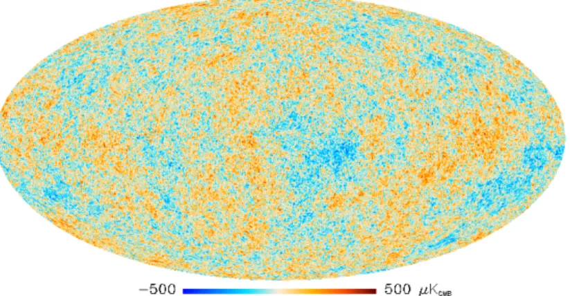
2.6 Mollweide projection of the CMB temperature fluctuations detected by team Planck. 27

2.7 The angular power spectrum of the CMB observed by the Planck satellite from

Planck collaboration et al. (2013). The red points stand for the data while the best fit model is displayed as a green line. The green shaded area indicates the cosmic variance magnitude. . . 28

2.8 The universe contents as derived by the preceding experiments on the left and by the Planck satellite on the right. Picture taken from ESA website (The scientific results can be found in Planck Collaboration et al. (2013c)). . . 29

(13)

List of Figures xii

2.9 Behaviour of r in function of nSfor di↵erent inflation models (colored lines) along

with the constraints coming from the Planck satellite and other observations (in shaded areas). Picture taken from Planck Collaboration et al. (2013a). . . 30

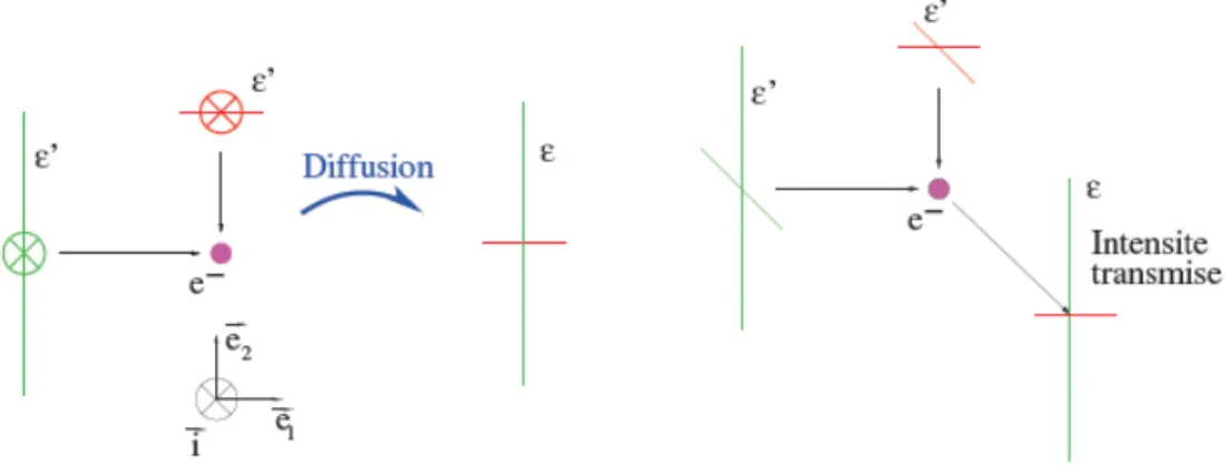
3.1 Transmitted intensity after scattering of photons presenting a quadrupolar anisotropy on a free electron. On the left panel, two incident perpendicular light beams with di↵erent intensity and the resulting intensity are depicted as projected on the plane orthogonal to the line of sight. The right panel displays the same scheme in pseudo-perspective. Picture taken from Ponthieu (2003). . . 32

3.2 Over-density in the primordial plasma. Around a given electron, the light intensity is quadrupolar. On the right panel, the polarisation pattern induced by the density perturbation. Image taken from Ponthieu (2003). . . 35

3.3 A gravitational wave passing through a circle of motionless test particles. On the upper (lower) panel, the gravitational wave have a ‘+’ (‘_{⇥’) polarisation. The} in-duced polarisation patterns corresponding to each gravitational wave polarisation are shown on the right planel. . . 35

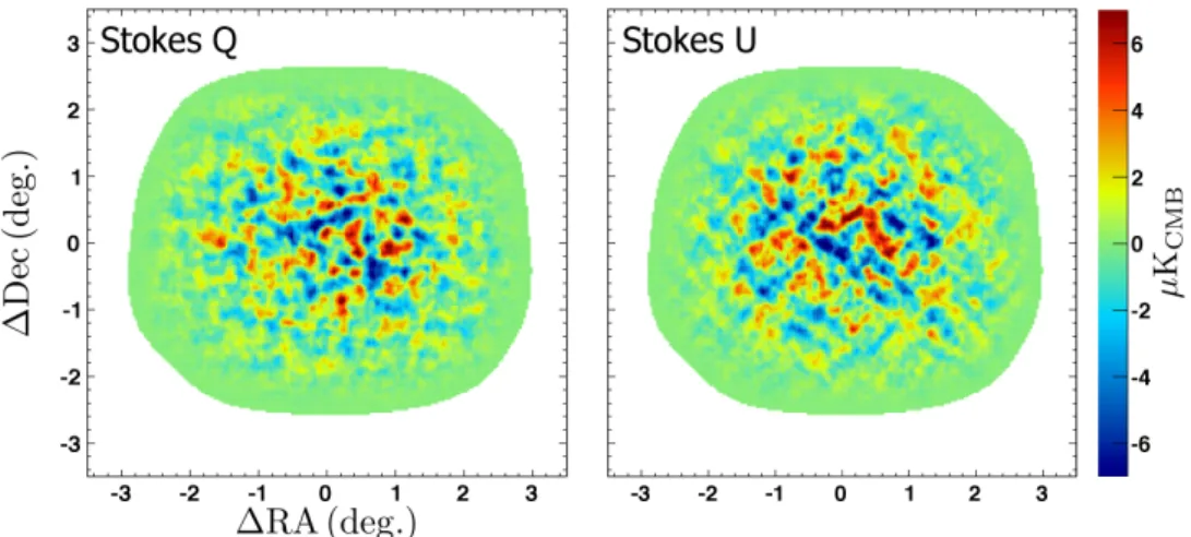
3.4 Q and U maps from The POLARBEAR Collaboration et al. (2014). . . 36

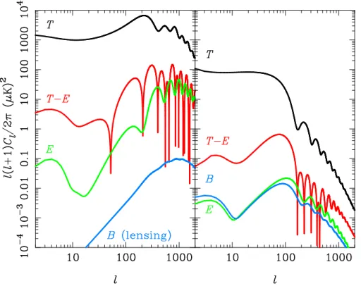
3.5 Scalar (tensor) contributions to the power spectra T , E and B modes and to the T E correlations on the left (right) panel (from Challinor (2013)). . . 40

3.6 T T , EE and T E power spectra from the ACTPol experiment. Picture taken from

Naess et al. (2014). . . 42

3.7 E modes power spectrum from the 7-yr WMAP experiment (from Larson et al.

(2011).) . . . 43

3.8 Earlier constraints and current measurements of the B modes power spectrum. . 43

4.1 The modulus of the convolution kernel F±(~n) for a given ~n such as ✓ = ⇡2 and

= 0, from Kim and Naselsky (2010). This filter is highly peak for cos(✓) = 0. . 64

4.2 Leakage map obtained using the standard pseudospectrum reconstruction. The

redder areas are the most aliased pixels. . . 67

4.3 Leakage map in the frame of the pure (zb) pseudospectrum reconstruction in the

left (right) panel. . . 67

4.4 Leakage map reconstructed via knpseudspectrum reconstruction. The map in

the left (right) panel is obtained using an apodised window function with an apodisation length of ✓apo= 0.5o (✓apo= 1o). . . 68

5.1 From left to right: the spin-0, spin-1 and spin-2 window functions of a spherical cap of radius 11o_{. The input signal is E modes from WMAP-5yr and the induced}

lensing B modes, assuming a primordial B modes signal with r = 0.05 and a noise level of 5.75µK-arcmin. Only the real part of the spin-1 ans spin-2 window functions are depicted. The top and middle rows show the spin-weighted optimized window function respectively in the pixel and the harmonic space, for the bin

`_{2 [20, 60]. The bottom row illustrates the window function computed with an}

analytic apodisation. The figures are taken from Grain et al. (2009). . . 76

5.2 The hopper system (from NERSC website). . . 78

5.3 Left panel : The binary mask of the fiducial satellite-like experiment designed from the polarised galactic mask of WMAP-7yr release with the corresponding polarised point sources catalogue removal. The (grey) red area is the (non) observed region of the sky. Right panel : same with no point sources removal. . . 82

5.4 Binary mask of the fiducial small scale experiment covering 1% of the sky. The

holes in the mask corresponds to masked point sources. The (grey) red area is the (non) observed region of the sky. . . 83

(14)

List of Figures xiii

5.5 Left panel: The pseudospectrum ˜CE!B

` obtained with no input B modes and E

modes power spectrum from WMAP-7yr best fit in solid black line obtained using the standard method for a large scale experiment. The coloured curves stand for the pseudospectrum ˜CB!B

` with no input E modes and a theoretical B modes

power spectrum for di↵erent values of r (r = 0.001, 0.01, 0.05, 0.1) along with the lensing contribution.Right panel: Same for the small scale experiment. . . 84

5.6 The pseudospectrum ˜CE!B

` obtained with no input B modes and E modes power

spectrum from WMAP-7yr best fit in solid black line obtained using the standard method for a large sky coverage without holes. The colored curves stand for the pseudospectrum ˜CB!B

` with no input E modes and a theoretical B modes power

spectrum for di↵erent values of r (r = 0.001, 0.01, 0.05, 0.1) along with the lensing contribution. . . 85

5.7 Pseudospectra built from leakage free methods in the case of a large scale experi-ment. Left panel: The pseudospectrum ˜CE!B

` obtained with no input B modes

and E modes power spectrum from WMAP-7yr best fit in solid (red) black line obtained using the pure (zb) method. The pseudospectrum ˜CB!B

` obtained with

no input E modes and a theoretical B modes power spectrum for r = 0.05 in dashed (red) black line obtained using the pure (zb) method. Right panel: The ratio ˜CE!B

` / ˜C`B!B between the B modes pseudospectrum with no B modes in

input and no E modes in input obtained in the kn method for di↵erent applied

masks (fsky = 72%, 70% and 66% in black, purple and blue respectively). . . 86

5.8 The pseudospectrum ˜CE!B

` obtained with no input B modes and E modes power

spectrum from WMAP-7yr best fit in solid black line obtained using the pure method for a large sky coverage without holes. The colored curves stand for the pseudospectrum ˜C`B!B with no input E modes and a theoretical B modes power

spectrum for di↵erent values of r (r = 0.001, 0.01, 0.05, 0.1) along with the lensing contribution. . . 87

5.9 Pseudospectra built from leakage free methods in the case of a small scale exper-iment. Left panel: The pseudospectrum ˜CE!B

` obtained with no input B modes

and E modes power spectrum from WMAP-7yr best fit in solid (red) black line obtained using the pure (zb) method. The pseudospectrum ˜C`B!B obtained with

no input E modes and a theoretical B modes power spectrum for r = 0.05 in dashed (red) black line obtained using the pure (zb) method. Right panel: The ratio ˜C`E!B/ ˜C`B!B between the B modes pseudospectrum with no B modes in

input and no E modes (r = 0.05) in input obtained in the kn method for di↵erent applied masks (fsky= 1%, 0.7% and 0.4% in black, blue and turquoise respectively). 88

5.10 The red crosses stand for the `-by-` reconstructed power spectrum using the stan-dard method for a large scale experiment. The input B modes power spectrum to be estimated is the solid black line. The dashed black line set a benchmark on the obtained uncertainties as it is the ideal mode counting ones. The error bars obtained using a binary mask, an analytic apodisation with an apodisation length ✓apo= 1o and ✓apo= 4o are displayed as red, blue and yellow curves respectively. 89

5.11 The red crosses stand for the `-by-` reconstructed power spectrum using the stan-dard method for a large scale experiment. The input B modes power spectrum to be estimated is the solid black line. The dashed black line set a benchmark on the obtained uncertainties as it is the ideal mode counting ones. The error bars obtained using a binary mask, an analytic apodisation with an apodisation length ✓apo= 7oand an harmonic variance-optimised window function are displayed red,

blue and yellow curves respectively.. . . 90

5.12 Power spectrum uncertainties on B-modes in dashed red line using the pure esti-mation for the case of a satellite-like experiment (fsky ⇠ 71%). The dashed black

line displays the ideal mode counting uncertainties. The sold red curve stand for the reconstructed B modes power spectrum of the input power spectrum in solid black curve. The grey shaded boxes represent the bins.. . . 91

(15)

List of Figures xiv

5.13 Power spectrum uncertainties on B-modes in dashed red line using the zb method thanks to an harmonic variance optimised window function for the case of a satellite-like experiment (fsky ⇠ 71%). The coloured dashed lines are the

ob-tained error bars for di↵erent lengths of apodisation ranging from ✓apo = 5o to

✓apo= 8o. The dashed black line displays the ideal mode counting uncertainties.

The sold red curve stand for the reconstructed B modes power spectrum of the input power spectrum in solid black curve. The grey shaded boxes represent the bins. . . 92

5.14 Power spectrum uncertainties on B-modes in dashed red, yellow and blue lines

using the kn method thanks to di↵erent mask (with fsky = 65%, 57%, 39%

re-spectively) in the case of a satellite-like experiment (fsky ⇠ 71%). The dashed

black line displays the ideal mode counting uncertainties. The coloured solid lines are the obtained reconstructed power spectra for the di↵erent e↵ective sky frac-tion. The input power spectrum is in solid black curve. The grey shaded boxes represent the bins. . . 93

5.15 The red crosses stand for the `-by-` reconstructed power spectrum using the stan-dard method for a large scale experiment without holes. The input B modes power spectrum to be estimated is the solid black line. The dashed black line set a benchmark on the obtained uncertainties as it is the ideal mode counting ones. The error bars obtained using a binary mask, an analytic apodisation with

an apodisation length ✓apo = 22o and an harmonic variance-optimised window

function are displayed red, blue and yellow curves respectively. . . 95

5.16 Summary of the power uncertainties obtained with a pure, zb and kn approach in dashed red, yellow ans blue curves respectively, in the case of a large scale survey without holes. The solid curve stands for the input power spectrum to be

estimated. The grey shaded boxes represent the binning of the power spectra. . . 95

5.17 Power spectrum uncertainties on B-modes in dashed red line using the zb method

for the case of a small scale experiment (fsky ⇠ 1%). The dashed black line

displays the ideal mode counting uncertainties. The sold red curve stand for the reconstructed B modes power spectrum of the input power spectrum in solid black curve. The grey shaded boxes represent the bins. . . 96

5.18 Power spectrum uncertainties on B-modes in dashed red line using the zb method thanks to an harmonic variance optimised window function for the case of a small scale experiment (fsky ⇠ 1%). The coloured dashed lines are the obtained error

bars for di↵erent lengths of apodisation ranging from ✓apo= 1oto ✓apo= 4o. The

dashed black line displays the ideal mode counting uncertainties. The sold red curve stand for the reconstructed B modes power spectrum of the input power

spectrum in solid black curve. The grey shaded boxes represent the bins. . . 97

5.19 Power spectrum uncertainties on B-modes in dashed red, yellow and blue lines

using the kn method thanks to di↵erent mask (with fsky = 0.86%, 0.72%, 0.42%

respectively) in the case of a small scale experiment (fsky⇠ 1%). The dashed black

line displays the ideal mode counting uncertainties. The colored solid lines are the obtained reconstructed power spectra for the di↵erent e↵ective sky fractions. The input power spectrum is in solid black curve. The grey shaded boxes represent the binning of the power spectra. . . 98

5.20 Error bars on the reconstructed angular power spectra for each of the three for-malisms (colored curves) alongside the naive (binned) mode counting estimate of such uncertainties for a small scale survey with inhomogeneous noise (from Grain et al. (2012)). . . 99

5.21 Power spectrum uncertainties on B-modes using cross-spectrum estimation for the case of satellite experiment with holes mimicking point sources-removal (fsky ⇠

71%). The red dashed line represents the uncertainties obtained via pure method, the blue dashed line corresponds to zb method and at last the yellow dashed dotted to the kn method. The dashed-black curve stand for mode counting estimate of the error bars.. . . 100

(16)

List of Figures xv

5.22 Power spectrum uncertainties for each of the three techniques for the case of a small-scale experiment with fsky ' 1%, a noise level of 5.75 µK-arc minute and

✓Beam = 8 arc minutes. Dashed-red, dashed-cyan and dashed-yellow curves are

respectively for the pure, zb and kn techniques. The dashed-black curve stand for mode counting estimate of the error bars. . . 101

6.1 In the left panel figures the binary mask for an observed sky fraction of 4%. The corresponding harmonic window function for r = 2 and `_{2 [2; 20] is displayed in} the right panel. . . 131

6.2 The signal-to-noise ratio for r = 0.2, 0.15, 0.1, 0.07, from top left to bottom right, using a naive mode-counting variance (in yellow), the pure estimation of the B

modes (in burgundy). The horizontal red line set the benchmark of 3 . . . 132

6.3 Same results as Fig. 6.2 with the signal-to-noise ratio displayed in each panel for all r. From left to right, (S/N)ris computed using the mode-counting approach,

the minimal variance quadratic estimator and the pure B modes estimation. The horizontal red line set the benchmark of 3 . . . 134

6.4 The left panel shows the inhomogeneous noise distribution for an experiment

covering 1% of the sky. The binary masks corresponding to an half sky and a full sky survey are displayed in the middle and right panel respectively. . . 135

6.5 The spin-0 PCG window function optimised in the bin ` 2 [60; 100] for small,

intermediate and large scale experiments in the left, middle and right panel re-spectively. . . 136

6.6 Variances reconstructed with the pure estimation on a theoretical CMB power

spectrum with r = 0.1 (in solid black line) in the case of a small scale survey (orange dashed curve), an intermediate scale survey (red dashed curve) and a full sky survey (burgundy dashed curve). . . 136

6.7 Signal-to-noise ratio on r with respect to r obtained for the fiducial small scale survey. The red (black) crosses connected by red (black) line are the obtained (S/N)rusing the mode-counting (pure) estimation of the covariance matrix in the

Fisher matrix. The horizontal red lines stand for 1 , 2 and 3 thresholds. . . . 137

6.8 Signal-to-noise ratio on r with respect to r obtained for the fiducial large scale survey. The red (black) crosses connected by red (black) line are the obtained (S/N)rusing the mode-counting (pure) estimation of the covariance matrix in the

Fisher matrix. The horizontal red lines stand for 3 . . . 137

6.9 Signal-to-noise ratio on r with respect to r obtained for the fiducial intermediate scale survey. The red (black) crosses connected by red (black) line are the obtained (S/N)rusing the mode-counting (pure) estimation of the covariance matrix in the

Fisher matrix. The horizontal red line stand for the 3 threshold.. . . 138

7.1 The CMB B modes (in black) power spectrum along with the T B (in red shades)

and EB (in blue shades) correlations for r(+) = 0.05, including the primordial

and lensing contributions. The three red and blue shaded curve correspond to

di↵erent values of : = 1 for a maximum parity breaking, = 0.5 and = 0.1.

The dotted lines stand for negative values of the odd correlations.. . . 142

8.1 The CMB BB power spectrum expected in the standard model with r = 0.05 in

black and the contribution from an helical PMF in dashed blue with nS = 2.99

and nH= 2.5. . . 173

(17)

List of Figures xvi

9.1 The signal-to-noise ratio of B modes detection for a satellite-like experiment. The solid black line stands for the one using the ideal mode-counting estimation of the variance. The red solid line is the one obtained from a pure B modes estimation along with pixel-based variance optimised window function. The yellow line displays the signal-to-noise ratio using the standard method to etimate B modes. The grey shaded areas set the 1 , 2 and 3 limits. The B modes have to be carefully estimated to ensure at least a 3 detection. (Taken from Fert´e et al. (2013)). . . 178

(18)

List of Tables

6.1 The minimal accessible r at 3 regarding the experimental set-up and the

esti-mation of the variance on the B modes reconstruction by linearly interpolating between the computed (S/N)r. . . 138

7.1 Signal-to-noise on r( )for di↵erent values of r(+)in the case of small-scale

(ballon-borne or ground-based) experiments, and using a mode-counting expression for the error bars on the angular power spectra reconstruction. . . 143

7.2 Signal-to-noise ratio on r( ), (S/N)r( ), as derived from a pure estimation of the

angular power spectra. (For a given value of r(+) and , the value of r( ) is

r( )= ⇥ r(+).) . . . 143

(19)

(20)

Introduction

Among all electromagnetic radiations surrounding us, there exists one particular light that orig-inates from the first moments of the Universe, today constituting the cosmic microwave back-ground (CMB). This light is composed of the oldest photons emitted in the Universe and is a valuable source of knowledge since it holds information about the formation and evolution of the Universe from the Big Bang up to now. Shortly after its discovery in 1964, the CMB was at the origin of many questions for instance, the origin of its statistical isotropy along with its tiny temperature fluctuations remain a mystery. Several theories have been proposed to solve these enigma but one is favoured for its simple explanation of most observed phenomena: the cosmic inflation. According to this paradigm, the Universe would have known a violent and ephemeral accelerated expansion about 10 30_{s after the Big Bang. Its existence would assert} the consistency of the standard model of cosmology and is only waiting for a firm experimental verification. It might seem impossible at first to observe such a distant epoch but cosmic inflation would have left perturbations of the space-time curvature, first under the shape of variations of the gravitational potential, but also under the shape of primordial gravitational waves. These are ripples of space-time which would have left imprints in the fluctuations of the CMB temperature and polarisation. By investigating its temperature and polarisation anisotropies, the CMB may hold the answers to the issues it raised.

Figure 1: During my PhD, I have focused my research on the CMB, a light much older than the light of any stars in the sky (picture by Marion Montaigne1₎

1_{tumourrasmoinsbete.blogspot.com}

(21)

Introduction ii However, the evidence of the primordial gravitational waves is so tiny that it can be hidden by the other sources of fluctuations in the CMB, except for one of the CMB polarisation modes: the B modes. The gravitational waves are indeed the only source of CMB B modes at large angular scales. The detection of the CMB B modes would therefore be a smoking gun for cosmic inflation. Their amplitude is however expected to be extremely low making their detection an instrumental and data processing challenge.

During my PhD thesis, my endeavour has consisted in developing, testing and validating new statistical methods to perform an accurate estimation of the CMB B modes in order to set thigh constraints on the cosmological parameters describing the very early universe. Due to its cosmological origin, the CMB is a peculiar observable since the signal itself contributes to the statistical uncertainties on its reconstruction, this is the so-called cosmic variance. This e↵ect becomes more puzzling in the case of a low signal such as the CMB polarisation because the E modes can contribute to the B modes signal. This e↵ect is known as the E-to-B leakage and leads to a laborious, if not impossible, reconstruction of the B modes. The leakage can strongly prevent from detecting the B-modes, even in an ideal noiseless case, because of the partial sky coverage. These uncertainties can however be statistically reduced thanks to clever methods correcting for this contamination. In that case, the CMB polarisation unveils clues about the first instants of the Universe, in particular about the inflation period.

As an introduction, I will first detail in partIthe formalism of polarisation, a key observable in astrophysics. I will then portray the CMB in the frame of the current standard model of cosmol-ogy, the ⇤CDM model. The CMB polarisation and its current detection status will be developed next. Afterwards, the partIIis dedicated to the reconstruction of the CMB polarisation power spectrum from the CMB maps. After introducing the formalism of the CMB statistics, I will demonstrate the efficiency of di↵erent pseudospectrum methods aiming at estimating accurately the uncertainties on the CMB power spectra. As a result, one of them proves to be the most efficient, so I use it as a tool to properly estimate the CMB B modes and derive the constraints on the primordial Universe (part III). In particular, I investigated the potential detection of the primordial Universe physics: the energy scale of the cosmic inflation, a parity violation and finally the existence of a primordial magnetic field, each of these issues being dealt with in sepa-rated chapters. I eventually conclude in partIVby summarizing the results of my PhD research and outlining my future projects.

(22)

Part I

Introduction: Light Polarisation

and the CMB

(23)

(24)

Chapter 1

Light Polarisation

During the 19th _{century, Malus and Arago have highlighted the light polarisation, a curious} be-haviour of light that they observed in peculiar crystals such as calcite. Ever since, the light polarisation is widely used for technological purposes such as 3D vision or remote sensing. It also explains numerous natural processes like the sky polarisation or the birefringence.

1.1 Polarisation Formalism in Optics

The light is classically described as a propagating electromagnetic wave. It is often reduced to its electric field component, from which the magnetic field is deduced thanks to the Maxwell equations. I present here the light description in the ideal but easier case of a monochromatic plane wave with a frequency ⌫ and a direction of propagation along its wave number ~k. In a ( ~ex, ~ey, ~ez) orthonormal system coordinate, the electric field representing such a wave propagating in the z direction is:

~

E(~r, t) = [Exex~ + Eyey]e~ i(kz 2⇡⌫t), (1.1) with Ei the complex amplitude of the electric field in the i-direction. In order to characterise this electromagnetic wave, the two main quantities to be measured are its intensity and its polarisation.

• Intensity

Measuring the electric field components at any moment would give a complete description of the electromagnetic wave. Nonetheless, in the case of high frequency light (in the order of hundreds of GHz) that are of interest to this thesis, the current detectors do not have high enough sampling frequency to have access to the electric field every fraction of microseconds. Nonetheless, the energy on a given surface during a given time lapse gives enough information to describe the

(25)

Chapter 1. Light Polarisation 4 wave. This measurable energy is the light intensity and is therefore defined as:

I(t) =⌦_|Ex|2↵_t+⌦|Ey|2↵_t, (1.2) where the bracketsh.it stand for time average.

The light intensity I(t) is an essential quantity that permits to characterise most optical phe-nomenons such as photometry, interferometry or polarimetry. It however eludes the light vecto-rial behaviour.

• Polarisation

The polarisation of the light holds the information on the vectorial structure of the electromag-netic field. More specifically, it defines the direction of its oscillations. Indeed, regarding the process at the origin of the light emission or in the way of the light path, the electromagnetic field can adopt a preferential direction with respect to the direction of propagation. A non-polarized light, such as the natural light, has its electric and magnetic fields varying too fast with respect to the sampling frequency of our best detectors and in an unpredictable direction. Nonetheless, there are processes that favour a peculiar direction of these electromagnetic oscillations. For instance, any kind of light outgoing from a linear polariser acquires one specific direction of the electric field oscillations given by the device which acts as a filter. The light polarisation may therefore give consequential information on the phenomenon from which it originates or on the medium in which the light is propagating. An interesting example which is only explained thanks to the polarisation is the birefringence. This peculiar e↵ect is due to anisotropies in the atomic distribution of some medium such as crystal quartz which has two favoured directions. This irregular arrangement implies local variations of the optical index. Consequently the di↵erent polarisation directions of the propagating light see di↵erent optical index of the medium. The di↵erent polarisations of the light thus refract in di↵erent directions. The light therefore emerges from the medium in two separated light beams perpendicularly polarised to each other as shown in Fig. 1.1. The birefringence is therefore tightly related to the light polarisation – and was at the origin of polarisation discovery.

Figure 1.1: An example of birefringence: the drawing of the sheep is split into two parts when looked through the birefringent crystal.

The light polarisation characterises the direction of the electric field oscillations, a general case of which is displayed in Fig. 1.3. It is thus an intrinsic property of the light ensuring an access

(26)

Chapter 1. Light Polarisation 5 to additional information on the nature of the light and the medium the light is going through. A specific formalism is therefore required to describe it.

Figure 1.2: A diagram of a polarised light. The black line stands for the direction of the electric field in time and its projection onto a plane is shown in yellow, drawing an ellipse: the

light is elliptically polarised (fromWikipedia polarisation page).

1.1.1 Fully polarized light

1.1.1.1 Jones formalism

A specific case of polarisation is the case of a totally polarized light: the electromagnetic field direction evolution is deterministic. Usually, in such a case, the Jones formalism is used to describe the light polarisation. The light can be characterized by a Jones vector while the properties of the medium it propagates in is embodied in the Jones matrix.

In this case, the equation (??) describing the behaviour of the electric field can be written as a vector ~E verifying: Re( ~E(~r, t)) = Re " Eox Eoyei # ei(kz 2⇡⌫t) ! = " Eoxcos(kz 2⇡⌫t) Eoycos( + kz 2⇡⌫t) # , (1.3)

with the phase between the two transverse components of the electric field and Eoiis the real amplitude of the i electric field component.

Following this expression, the Jones vector is defined as: ~ J = " Jx Jy # = " Eox Eoyei # . (1.4)

(27)

Chapter 1. Light Polarisation 6 By reformulating Eq. (1.3) and combinating the two components of the electric field, an equation giving insight on the evolution of each component Ei of the electric field is obtained:

E2 x E2 ox + E 2 y E2 oy 2Ex Eox Ey

Eoy cos( ) = sin( )

2_. _(1.5)

This equation is the equation of an ellipse inscribed in a rectangle of side width 2Eoxand 2Eoy, as shown in Fig.1.3. The cross term in ExEy indicates that the ellipse is rotated. The polarisation is said to be elliptic: the electric field vector draws an ellipse over the time. The polarisation is either left- or right-handed depending on the sign of the phase shift . If > 0, the polarisation is then left-handed (trigonometric orientation) and vice versa.

x" y" 2Eox 2Eoy ." z  E(M, t)

Figure 1.3: The ellipse drawn by the evolution of the electric field ~E(M, t) in time when the light is elliptically polarised (see Eq. (1.5)).

From the general case of an elliptic polarisation, two peculiar cases come out: the linear and circular polarisations. In the former case, the electric field oscillations are contained in a plane and its components verify Ex

Ey = cste. The Jones vector of a light linearly polarised along (Ox) is

therefore written: ~J = "

1 0

#

. The electric field direction of a circularly polarised light follows a circle in time. The Exand Eycomponents of the electric field are therefore equal and the phase is equal to±⇡

2. Thus, the Jones vector of right-handed circular polarisation is: ~J = 1 p 2 " 1 i # because here = ⇡ 2. 1.1.1.2 Poincar´e Sphere

The Poincar´e sphere is a tool introduced inPoincar´e et al.(1892) to easily describe the polarisa-tion state of the light and its modificapolarisa-tion. It is very useful since it enables to quickly derive the resulting polarisation state of light after going through a polarising device such as a waveplate. As shown in figure1.4, the coordinate system (Ox0y0z0) in which the electric field is measured is rotated by an angle ↵ with respect to the proper coordinate system (Oxyz) of the polarisation ellipse, with z = z0_{. Therefore, the electric field transforms as:}

(

Ex0 = Excos(↵) + Eysin(↵),

Ey0 = Eycos(↵) Exsin(↵),

(1.6)

(28)

Chapter 1. Light Polarisation 7 x" y" x'" y'" α O"  E(M, t)

Figure 1.4: The coordinate change between (x, y) and (x0, y0), the proper axes of the polari-sation ellipse drawn by the electric field ~E(M, t) evolution.

Thus, the electric field in the (Oxyz) system is: (

Ex= Ex0cos(↵) Ey0sin(↵),

Ey= Ex0sin(↵) + Ey0cos(↵).

(1.7)

In (Ox0_y0_z0_{) the equation (}_1.5_{) of the polarisation ellipse consequently writes:} Ex02 ✓_cos(↵)2 E2 ox +sin(↵) 2 E2 oy

2 cos(↵) sin(↵) cos( ) EoxEoy ◆ +Ey02 ✓_sin(↵)2 E2 ox +cos(↵) 2 E2 oy

2 cos(↵) sin(↵) cos( ) EoxEoy ◆ +2E0xE0y ✓ cos(↵) sin(↵) ✓ 1 E2 ox + 1 E2 oy ◆ cos(↵) EoyEox ◆ cos( ) = sin(↵). (1.8)

In this coordinate system (O0x0y0z0), the ellipse is not rotated as its proper axes are along (O0x0) and (O0_y0_{). The coefficient of the cross term in bold letters of Eq. (}_1.8_{) must therefore be set} equal to zero. We therefore obtain a relation between ↵ and the characteristics of the polarisation ellipse Eoi and :

tan(2↵) = 2 EoxEoy E2

ox Eoy2

cos( ). (1.9)

The semi-major axis a and semi-minor axis b of the ellipse write: (

a2_{= E}2

oxcos ↵2+ Eoy2 sin ↵2+ 2EoxEoycos ↵ sin ↵ cos , b2_{= E}2

oxsin ↵2+ E2oycos ↵2 2EoxEoycos ↵ sin ↵ cos .

(1.10)

Instead of using the three previously derived parameters a, b and ↵, the ellipse can be described by the three following parameters:

- the light beam intensity I = E2

ox+ Eoy2 = a2+ b2;

- the azimuth angle ↵ that characterises the tilt of the polarisation ellipse and varies from 0 to ⇡;

- the ellipticity ✏ given by: tan ✏ =±b

a, representing the width of the ellipse. ✏ varies from ⇡ 4 to ⇡₄. Fig. 1.5illustrate a generic elliptic polarisation showing the ↵ and ✏ angles.

(29)

Chapter 1. Light Polarisation 8

x" y"

α

ε

Figure 1.5: The ellipticity, ✏, and azimuth, ↵, angles of the polarisation ellipse.

These three parameters I, ↵ and ✏ therefore utterly describe the light polarisation. The Poincar´e sphere is a sphere of centre O, unity radius and axis OX, OY and OZ, where the polarisation state is represented as a point which coordinates depend on the three parameters.

By convention, the (OXY ) plane is the plane with ✏ = 0 and the (OXZ) the one with ↵ = 0 as illustrated in Fig.1.6. The polarisation state of a totally polarised light with an azimuth ↵ and an ellipticity ✏ is thus represented by a point M(X’,Y’,Z’) at the surface of the Poincar´e sphere whose coordinates are defined as:

8 > > < > > : X0_{= cos 2↵ cos 2✏,} Y0= sin 2↵ cos 2✏, Z0 _{= sin 2✏.} (1.11) X" Y" Z" M(X’,Y’,Z’)"

Figure 1.6: An elliptical polarisation of azimuth ↵ and ellipticity ✏ placed on the Poincar´e sphere.

By convention, the upper hemisphere is the location of the left-handed polarisation, while the bottom is the one of the right-handed polarisation. The two particular cases of circular and linear polarisation evoked above can thus be placed on the Poincar´e sphere. For a fully polarised beam light with intensity I:

- a right-handed circularly polarised light is represented by M (0, 0, 1);

- a light linearly polarised with an angle ↵ is represented by M (cos(2↵), sin(2↵), 0).

The Jones formalism is a useful formalism to describe a fully polarized light and it can be easily pictured thanks to the Poincar´e sphere. Nonetheless, it cannot be used to describe a partially polarised light which is however the case of most polarised electromagnetic waves.

(30)

1.1.2 Partially polarized light

1.1.2.1 Stokes parameters

Between the two cases of a fully polarised and an unpolarised light lies the case of the partially polarised light that concerns most radiations. In this more realistic case, the Jones vector no longer has a deterministic behaviour and is therefore not appropriate anymore. Proposed by Stokes in 1852, the Stokes parameters are very handy quantities which contain all the needed information about the light to accurately analyse its polarisation.

The Stokes parameters can be deduced from the so-called coherence matrix which encodes for the covariance of the randomly evolving Jones vector.

However, as done inCollett(1992), the Stokes parameters can be easily derived from an empirical perspective. The equation (1.5) describing an elliptical polarisation is valid in the case of fully polarised light. The typical time scale involved here – such as the time for the electric field to draw the ellipse – is nonetheless in the order of 10 15_{s. Thus the polarisation ellipse remains} elusive to our detectors. Therefore, in the same way we have introduced the intensity, we may want to transcribe the polarisation ellipse characterised by the ✏, ↵ variables into observable quantities.

Using current detectors gives access to the electric field integrated over a time period. We therefore need to integrate in time the equation (1.5) of a monochromatic wave propagating in the z-direction with an elliptical polarisation. As the electric field is periodic, it is equivalent to average it in time over one oscillation:

⌦ Ex(t)2↵ t E2 ox + ⌦ Ey(t)2↵ t E2 oy 2hEx(t)Ey(t)it

EoxEoy cos( ) = sin( )

2_, _(1.12) with _hEiit = lim T!1 1 T R1

0 Ei(t)dt, i = x, y. For a monochromatic wave propagating in the z-direction, whose expression is given by Eq. (1.3), we obtain: _hEiit = ₂1Eoi2 and hEiEjit =

1

2EoxEoycos( ).

Multiplying by 4EoxEoy and inserting the expression of hEiitin the above equation gives: 4E2

oxEoy2 4E2oxEoy2 cos2( ) = 4Eox2 Eoy2 sin2( ). (1.13)

We thus obtain the canonical expression:

(Eox2 + Eoy2 )2 (Eox2 Eoy2 )2 (2EoxEoycos( ))2= (2EoxEoysin( ))2. (1.14)

By rewriting the previous equation (1.14) in the form: S02 S12 S22= S32, we deduce: 8 > > > > < > > > > : S0= Eox2 + Eoy2 , S1= E2 ox Eoy2 , S2= 2EoxEoycos( ), S3= 2EoxEoysin( ). (1.15)

(31)

Chapter 1. Light Polarisation 10 These four quantities are the so-called Stokes parameters and fully describe any type of light beam. The first Stokes parameter S0 is, compared to Eq. (1.2), the total intensity of the light and is linked to the other parameters via the relation: S2

0 > S12+ S22+ S23, the equality being the case of a fully polarised light. Also, from these parameters, the polarisation degree P is defined. It quantifies the ratio between the polarised contribution Ipolwith respect to the total intensity:

P = Ipol Itot = p S2 1+ S22+ S32 S0 . (1.16)

P is consequently ranging from 0 for an unpolarised light to 1 for a totally polarised light. A partially polarised light has its polarisation degree such as 0 < P < 1.

In the general case of a light beam described with a complex amplitude as in Eq. (??), the same

reasoning gives: ₈ > > > > < > > > > : S0= ExE⇤ x+ EyEy⇤, S1= ExEx⇤ EyEy⇤, S2= ExE⇤ y+ EyEx⇤, S3= i(ExE⇤ y EyEx⇤). (1.17)

From these parameters, the so-called Stokes vector are built:

S = 0 B B B B @ S0 S1 S2 S3 1 C C C C A. (1.18)

The Stokes parameters are also denoted Q, U and V , corresponding to S1, S2and S3respectively. On the one hand, the (Q, U ) Stokes parameters describe the linear polarisation and are tightly coupled because U is equivalent to the Q quantity but defined in a coordinate system rotated by 45o_{. On the other hand, the V Stokes parameter characterises the circular polarisation. Thus,} for three peculiar examples of light with intensity I and polarisation degree P , the Stokes vectors give:

- S = I (1 0 0 0)T if unpolarised;

- S = I (1 0 0 P )T if right-handed circularly polarised; - S = I (1 P 0 0)T if linearly polarised along (Ox); whereT _{denotes the transpose operation.}

Any polarisation state can be described by the linear combination of a circularly polarised light and a linerly polarised light. The (Q, U, V ) Stokes parameters thus ensure an utter description of the light polarisation. The Jones formalism is used in the peculiar case where P = 1.

(32)

Chapter 1. Light Polarisation 11 1.1.2.2 Poincar´e sphere

The reduced Stokes vector is defined as:

~s = 0 B B @ S1 S2 S3 1 C C A . (1.19)

The norm of this vector ~s is:

|~s| = q

S2

1+ S22+ S32= P Itot, (1.20)

by definition of the polarisation degree P .

The expression of the azimuth parameter ↵ in equation (1.9) and the properties of the semi-axis a and b give a relation between the Stokes parameters and the characteristics of the polarisation

ellipse: ₍ tan(2↵) = S2 S1, sin(2✏) = S3 S0. (1.21)

From these relations, we deduce the following expressions for the reduced Stokes vector:

s = 0 B B @ Q U V 1 C C A = P Itot 0 B B @ cos(2↵) cos(2✏) sin(2↵) cos(2✏) sin(2✏) 1 C C A . (1.22)

From this reduced Stokes vector, it is noticeable that ~s sets the location of the polarisation state inside the Poincar´e sphere at a distance P from the centre. Moreover, it is the generalisation of Eq. (1.13) for any polarisation degree.

For instance a partially linearly polarised light with an azimuth angle ↵ and a polarisation degree P will be a point M inside the Poincar´e sphere whose coordinates are: M (P cos 2↵, P sin(↵), 0). In the specific case of an unpolarised light, M is located at the center of the sphere (P = 0).

1.1.2.3 Stokes parameters properties

By measuring a polarised light beam, we implicitly choose a reference coordinate system (O ~exey~ez)~ where the intensity parallel or orthogonal to (Ox) is measured, in order to measure the Stokes parameters. Now we define a coordinate system (O ~ex0ey~0ez~0) such as:

8 > > < > > : ~ ex0 = cos( ) ~ex+ sin( ) ~ey, ~

ey0 = sin( ) ~ex+ cos( ) ~ey,

~

ez0 = ez,~

(1.23)

(33)

Chapter 1. Light Polarisation 12 The electric field in the rotated frame is then:

8 > > < > > :

E00x = cos( )E0x+ sin( )E0y, E0y0 = sin( )E0x+ cos( )E0y,

E0z0 = E0z.

(1.24)

And the intensity measured in the system (O ~ex0ey~0ez~0) is:

I0= E0x2 0+ E0y20 = E0x2 + E0y2 = I. (1.25) As expected, the intensity being an intrinsic scalar property of the light, it does not depend on the choice of the coordinate system.

Moreover, because it characterises the circularly polarised part of the light, the Stoke parameter V does not vary when rotating the reference frame:

V0= V. (1.26)

From their definition, the other Stokes parameters Q and U are transformed under this rotation

following: ₍

Q0= cos(2 )Q + sin(2 )U,

U0₌ _{sin(2↵)Q + cos(2↵)U.} (1.27)

This shows the peculiar feature of the (Q, U ) Stokes parameters: they are dependent upon the coordinate system in which they are defined, contrary to the intensity or V . We therefore have to be very careful to the way we compute the Stokes parameters and we will see in Chapter3

how this problem is circumvent in cosmology.

To conclude, the Stokes parameters are very useful as they are linear combinations of measur-able quantities. The next section is dedicated to the method of detection of these polarisation parameters. Some examples of application of the polarisation features in the field of astrophysics will be presented.

1.2 Polarisation Detection

1.2.1 Instruments

Various materials, either natural or artificial, modify the polarisation state of the light. The most common is the linear polariser: it transforms any light into a light linearly polarised in the direction of its axis. The figure1.7 displays this e↵ect in the case of a polariser, pictured as a grid, with its axis along the vertical. Its action on the Poincar´e sphere defined in the coordinate system (OXY Z) is the projection of any point M of the sphere in a point M0 in the (OXY ) plane. More precisely, M0 has the coordinate (cos(2↵), sin(2↵), 0) with ↵ the angle made by the polariser axis with respect to (OX).

(34)

Figure 1.7: The e↵ect of a linear polariser pictured as grid on an incident unpolarised light: the outgoing light is linearly polarised (fromWikipedia polariser page).

Two other kinds of useful analysers are the half-wave and the quarter-wave plates. Their prin-ciple lies in introducing a phase shift of ⇡ and ⇡₂ (for the half-wave and quarter-wave plates respectively) between the two orthogonal components of the incident light. On the Poincar´e sphere, it induces a rotation of an angle equal to the phase shift around the axis of the wave plate. These wave plates are widely used for the detection of the light polarisation.

Finally, the devices dedicated to the detection of light polarisation are well known. We can therefore have access to the information held in the light polarisation which are complementary to the usual observed quantity I(t), the light intensity. The polarisation indeed probes various physical processes up to the microscopic scale, such as the ones I will explain in the following section.

1.2.2 Polarisation in astrophysics

In the field of astrophysics, the key property involved in polarisation studies is that any light reflecting on a surface gives an outgoing polarised light. The induced polarisation can therefore be a crucial source of information on distant medium.

Figure 1.8: The Crab Nebula as seen from the Hubble telescope. Its polarisation is well known and is therefore a calibration source for CMB experiments (fromAPOD).

(35)

Chapter 1. Light Polarisation 14 The light polarisation is an observable of choice for planetary science. First, in the same way our sky is polarised due to light scattering, Venus atmosphere is polarised. As this planet surface is otherwise unobservable by current instruments, its atmosphere emission is thus crucial for the study of this planet. Its polarimetry is consequently of interest as shown in Hansen and Hovenier(1974). The same reasoning can be applied to Jupiter-like exoplanets as inStam et al.

(2004). Their polarised emission can indeed help to detect and characteris them. This statement has driven the construction of the promising zimpol instrument (which specifications are found in Thalmann et al. (2008)) included in the sphere exoplanet imager, recently installed at the Very Large Telescope. Moreover, other astrophysical objects such as nebula have also a polarised emission. It originates from the reflection of the light from the inner object on the surrounding matter. For instance, the Crab nebula, pictured in Fig. 1.8, has been intensively observed and its polarisation is now very well known. It is thus a convenient astrophysical object for the calibration of CMB experiments such as the polarbear experiment.

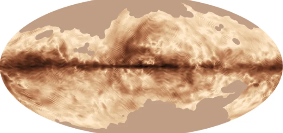
Furthermore, the dust is an appropriate example of the microphysics information revealed by the polarised emission. The dust is indeed prominent in the interstellar medium of our galaxy and give access to the process responsible for stellar formation. As a consequence, its constitution and evolution are currently under scrutiny. The interstellar dust is polarised under the e↵ect of the galactic magnetic field. It is thus a key observable to better understand the magnetic field at galactic scales. In particular, in Planck Collaboration et al. (2014), the Planck team has released a map of the magnetic field in the Milky Way shown at Fig. 1.9. However, the dust polarisation is also a contaminant for the study of cosmological observable as developed in Chapter4. Therefore, for the understanding of the interstellar medium and also for cleanliness of the cosmological surveys, a perfect knowledge of the dust polarisation is crucial. Also, the ionised medium surrounding stars can be polarised by scattering.

Figure 1.9: The magnetic field in the Milky Way deduced from the dust polarisation as seen from the Planck satellite (fromPlanck Collaboration et al.(2014)).

To conclude, several physical phenomenons including scattering, reflexion or magnetic field, can induce light polarisation. Polarimetry is thus a powerful observational tool in astrophysics as it can probe the microscopic scales physics of astrophysical objects. In order to share the knowledge of the di↵erent communities using this key observable, an e-COST (European Cooperation in

(36)

Chapter 1. Light Polarisation 15 Science and Technology) has been dedicated to the polarisation1_{in astrophysics and cosmology} showing that the polarisation detection is decisive in our understanding of the Universe.

Conclusion

The light polarisation is of great importance for astrophysics and cosmology as it reveals a multitude of information on the underlying processes such as the interstellar dust properties for instance. The cosmic microwave background being one of the main cosmological probes, its polarisation might tell us a lot about our Universe. In the next chapter, I will present the current standard model of cosmology followed by a close look at the cosmic microwave background.

(37)

(38)

Chapter 2

The Cosmic Microwave

Background in the Frame of

⇤CDM Model

The existence of a remaining light from the first instants of the Universe was predicted by Gamow, Alpher and Bethe in the late 40s. An indirect insight of this relic light has been found by McKel-lar (1941) who studied the interestellar molecules. However, a real asset would have been a direct detection of this cosmological background. After Dicke’s attempts for its observation, it was unexpectedly discovered byPenzias and Wilson(1965). The existence of a cosmic microwave backgroung radiation was therefore firmly confirmed, leading the way to numerous observations for its utter characterisation. Meanwhile, this detection has permitted to establish the model of the Hot Big Bang on observational ground.

2.1 The ⇤ CDM Model

Our current description of the Universe succeeds in explaining the origin of the large scale structures, the presence of relics contents such as photons or atoms, the dynamics of the Universe and its evolution. The observations are well outlined by the standard model but the underlying microphysics remains under scrutiny.

2.1.1 A dynamic Universe

Universe in expansion

By virtue of his observation, Hubble(1929) has asserted that the furthest are the galaxies the faster they recede. He has indeed measured the distance of galaxies thanks to the Cepheids