HAL Id: hal-02360894
https://hal.archives-ouvertes.fr/hal-02360894
Submitted on 13 Nov 2019
HAL is a multi-disciplinary open access
archive for the deposit and dissemination of
sci-entific research documents, whether they are
pub-lished or not. The documents may come from
teaching and research institutions in France or
abroad, or from public or private research centers.
L’archive ouverte pluridisciplinaire HAL, est
destinée au dépôt et à la diffusion de documents
scientifiques de niveau recherche, publiés ou non,
émanant des établissements d’enseignement et de
recherche français ou étrangers, des laboratoires
publics ou privés.
Clumpiness of the interstellar medium in the central
parsec of the Galaxy from H2 flux-extinction correlation
A Ciurlo, T. Paumard, D. Rouan, Y. Clénet
To cite this version:
A Ciurlo, T. Paumard, D. Rouan, Y. Clénet. Clumpiness of the interstellar medium in the central
parsec of the Galaxy from H2 flux-extinction correlation. Astronomy and Astrophysics - A&A, EDP
Sciences, 2019, �10.1051/0004-6361/201731763�. �hal-02360894�
Astronomy
&
Astrophysics
https://doi.org/10.1051/0004-6361/201731763 © ESO 2019
Clumpiness of the interstellar medium in the central parsec of the
Galaxy from H
2
flux–extinction correlation
A. Ciurlo
1,2, T. Paumard
1, D. Rouan
1, and Y. Clénet
11LESIA, Observatoire de Paris, PSL Research University, CNRS, Sorbonne Universités, UPMC Univ. Paris 06, Univ. Paris Diderot,
Sorbonne Paris Cité, 5 place Jules Janssen, 92195 Meudon, France e-mail: thibaut.paumard@obspm.fr; daniel.rouan@obspm.fr
2University of California Los Angeles, 430 Portola Plaza, Los Angeles, CA 90095, USA
e-mail: ciurlo@astro.ucla.edu
Received 12 August 2017 / Accepted 26 October 2018
ABSTRACT
Context. The central parsec of the Galaxy contains a young star cluster embedded in a complex interstellar medium. The latter mainly
consists of a torus of dense clumps and streams of molecular gas (the circumnuclear disk) enclosing streamers of ionized gas (the Minispiral).
Aims. In this complex environment, knowledge of the local extinction that locally affects each feature is crucial to properly study and
disentangle them. We previously studied molecular gas in this region and inferred an extinction map from two H2 lines. Extinction
appears to be correlated with the dereddened flux in several contiguous areas in the field of view. Here, we discuss the origin of this local correlation.
Methods. We model the observed effect with a simple radiative transfer model. H2emission arises from the surfaces of clumps (i.e.,
shells) that are exposed to the ambient ultraviolet (UV) radiation field. We consider the shell at the surface of an emitting clump. The shell has a varying optical depth and a screen of dust in front of it. The optical depth varies from one line of sight to another, either because of varying extinction coefficient from the shell of one clump to that of another or because of a varying number of identical clumps on the line of sight.
Results. In both scenarios, the model accurately reproduces the dependence of molecular gas emission and extinction. The reason
for this correlation is that, in the central parsec, the molecular gas is mixed everywhere with dust that locally affects the observed gas emission. In addition, there is extinction due to foreground (“screen”) dust.
Conclusions. This analysis favors a scenario where the central parsec is filled with clumps of dust and molecular gas.
Separat-ing foreground from local extinction allows for a probe for local conditions (H2 is mixed with dust) and can also constrain the
three-dimensional (3D) position of objects under study.
Key words. Galaxy: center – dust, extinction – infrared: ISM – ISM: structure – techniques: imaging spectroscopy
1. Introduction
The central parsec of the Galaxy hosts a supermassive black hole (Sgr A*;Lynden-Bell & Rees 1971). In the immediate environ-ment of Sgr A*, there is a very young star cluster (Becklin & Neugebauer 1968) emitting strong ultraviolet (UV) radiation (Martins et al. 2007). This region exhibits two main structures of interstellar medium (ISM): the circumnuclear disk (CND), com-posed of dust and neutral gas (Becklin et al. 1982), and the HII
region Sgr A West (the Minispiral), consisting of dust and ion-ized gas (Lo & Claussen 1983). The ISM, and particularly its molecular phase, plays an important role in Galaxy evolution, fueling star formation and the growth of super massive black holes.
At optical wavelengths, the Galactic center is obscured by an extinction of AV ∼30 magnitudes because of diffuse dust along
the line of sight (Rieke et al. 1989). Later works (Fritz et al. 2011;
Gao et al. 2013) suggest that the extinction might be even higher. To properly analyze any component (star, gas, dust) in terms of photometry or morphology, extinction correction is crucial. In the past decade, various authors have addressed the question of the local variations of the extinction in the Galactic center and have traced the extinction map of this region using different
tracers (Scoville et al. 2003;Schödel et al. 2010;Fritz et al. 2011, among others).
Two important aspects must be considered: the behavior of the extinction law as a function of the wavelength and the local variations of the spectral extinction coefficient. These local variations of the extinction are introduced by the specific envi-ronment to which the emitter is subjected. Local extinction must be estimated to distinguish between variations of brightness caused by extinction and by the intrinsic source.
Even though the bulk of extinction is foreground and amounts to 2.5 mag at K-band (Fritz et al. 2011), most of the vari-ation in extinction is local. For instance,Paumard et al.(2004) showed that the dust contained in the Eastern Bridge of the Minispiral is responsible for 0.76 mag of extinction at K of the Northern Arm.Schödel et al.(2010) obtained a AKsmap,
show-ing local variations reachshow-ing 1 mag, with a typical dispersion of 0.5 mag.
One must point out that extinction correction of an object is dependent on its three-dimensional position. Extinction maps are of limited use because of the fact that the various emitters – stars, ionized gas, and molecular gas – are not at the same 3D position and not at the same line of sight position with respect to the absorbing dust. This is also true for any source used as a
A&A 621, A65 (2019) AKs [mag] log 10 [F / 10 -1 9 W /s/ m 2/a rcse c 2]
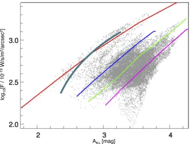
Fig. 1.H21-0 S(1) line dereddened flux against AKsfor each pixel in
the SPIFFI field of view.
probe to evaluate the local extinction. For this reason it is better, when possible, to evaluate the extinction variations directly from the emitter that is being studied.
In Ciurlo et al. (2016) we analyzed H2 in the central
par-sec. To do so, we used a spectro-imagery datacube obtained by SPIFFI (Tecza et al. 2000) at the VLT in 2003 (Eisenhauer et al. 2003). The observed field of view is 3600× 2900, with a
spec-tral resolution R = 1 300 in the near-infrared (NIR). The specspec-tral range of the observation covers several H2lines.
To properly describe the gas morphology, we built an extinc-tion map from two of the observed lines. We considered 1-0 S(1) and 1-0 Q(3) transitions at 2.1218 and 2.4236 µm, respectively, which correspond to transitions arising from the same upper level. We derived the extinction map and used it to deredden the flux map of the H2line 1-0 S(1). The description of the dataset,
the method used, the derived extinction and the whole procedure can be found inCiurlo et al.(2016). In the current paper, we con-centrate on the relation between the extinction and line flux maps to evaluate the effects of local extinction.
In Sect.2 we show that the dereddened flux map and the extinction map show local correlations. In Sect.3 we propose a phenomenological model to account for the observed effects. This model describes the observations well, as we show in Sect. 4. In Sect. 5we discuss how this analysis shows that H2
is everywhere mixed with dust in the central cavity of the CND, where it is arranged in multiple (up to 20) small-scale clumps.
2. Observation of the flux–extinction correlation
In Ciurlo et al.(2016) the extinction AKs is derived by simply
assuming that the primary source is an optically thin layer of hot H2. This is assuming that the ratio of the primary fluxes of
lines Q(3) and S(1) is simply given by their Einstein coefficients and wavelengths (AQ3/AS 1·λS 1/λQ3). The obtained dereddened
flux map and AKs map (Ciurlo et al. 2016, Fig. 5) appear
corre-lated: the flux is high where extinction is high. In order to check this apparent correlation, we plotted the logarithm of the dered-dened flux of the 1-0 S(1) line against AKsfor each pixel in the
field (Fig.1). A correlation between flux and AKswould appear
as a continuous monotonically rising line on this plot. However, the plot does not show a single line, but rather several elongated groups of data points. One can distinguish at least four sets of
AKs [mag] log 10 [F / 10 -1 9 W /s/ m 2/a rcse c 2]
R.A. Offset from Sgr A* [ arcsec ]
D e c. O ff se t fro m Sg r A* [ a rcse c ] −10 0 10 −10 0 10
Fig. 2. Top panel: as in Fig.1. The groups of correlated points are identified by different colors. Bottom panel: spatial distribution of the correlated group of points. Each pixel is colored according to the set it belongs to. White pixels indicate where the green and magenta groups overlap and black pixels where there is no coverage by any of the selected groups. Sgr A* is indicated by the white cross. Red symbols indicate the position of Wolf-Rayet stars: stars for type WN and trian-gles for type WC (Paumard et al. 2006catalog). The solid black squared areas indicate regions where we lack observations. GCIRS 7 is covered by the central black square.
groups of points in the correlation plot, as if there were no global correlation, but instead several local correlations.
To investigate these correlations, we selected five apparently correlated groups by eye and drew possible correlation curves through them. Points closer than a chosen distance to the curve are assigned to that group and colored with a tag color. The result of this assignment procedure is shown in Fig.2(top). This pro-cedure depends on two arbitrary parameters: (1) the correlation curve, drawn arbitrarily on the distribution of points, chosen to represent the different groups; and (2) the maximum distance to the curve, which is chosen in order to cover a maximum of points that seem related to the curve while avoiding any overlap between distinct curves.
This approach does not necessarily address all points and some of them remain black on the plot. Each colored point of the correlation plot corresponds to a SPIFFI pixel in the dereddened S(1) flux image which can be painted with the same color in the
spatial plane. The result is a map that shows where the differ-ent correlated sets are distributed (Fig.2, bottom). Interestingly, each set corresponds to a continuous area on the SPIFFI field and therefore strengthens the idea that the observed correlation is real. We tried selecting curves along other random directions to verify our choice of parallel increasing curves. This results in more randomly scattered regions in the SPIFFI field of view. The combination of almost parallel curves originally chosen is the one that leads to the most contiguous areas on the SPIFFI field of view.
In summary, we observe two effects: extinction correlates with flux and this correlation splits into several distinct areas.
3. Radiative-transfer toy model
If one considers just one of the colored curves obtained in the correlation plot, the problem is to understand how flux and extinction could be correlated. This positive correlation means that the larger the extinction, the higher the flux. It implies that the emitting material (i.e., the hot molecular gas) is located at the same spatial location as the absorbing material (i.e., dust). When the total thickness of the medium increases, the total amount of photons produced increases, but at the same time the average extinction that affects these photons increases as well. The above argument applies for each correlated set of points.
All correlation curves show the same slope but are shifted toward higher or lower values of the extinction. An important point is that separated sets correspond to distinct areas on the observed field of view. The reason for this separation might reside in the difference in large-scale foreground extinction along the line of sight between each of these areas. This extinc-tion acts as a non-emitting “screen” which attenuates radiaextinc-tion from the emitting material. Each of the painted areas corre-sponds to a medium which is subjected to a specific foreground extinction.
Starting from these qualitative ideas, we propose a sim-ple phenomenological model to account for the above-described extinction-flux correlation.
To build a phenomenological “toy” model, we also take into account the fact that we know that the UV radiation is very rapidly absorbed by H2through Lyman and Werner bands. This
happens at the surface of clumps that are optically thick for
UV. Therefore, the hot H2 NIR emission arises from a thin
shell (∼1/100 of the whole clump length), at the surface of gas clumps (Ciurlo et al. 2016), where dust is mixed with the H2molecules.
As illustrated in Fig.3, we assume an emitting shell (at the surface of a clump), composed of homogenous medium. In the shell, hot gas and dust are mixed and in front of this emitting shell we assume a purely absorbing screen. In the medium com-posing the shell, we assume the excitation temperature to be constant. Thus, the optical depth along the geometrical thickness in the medium is given by
τλ(x) = αλ· x, (1)
where αλ is the absorption coefficient per unit of length and x
is the path length. This extinction is entirely due to dust since self-shielding by H2itself is totally negligible (see AppendixA).
Along the line of sight to the observer, the dust screen absorbs part of the shell emission, adding an optical depth τ0. Both
opti-cal depths depend on the wavelength λ according to the same extinction law. dx 0 L0 L x screen cloud ho t H2 s he ll
Fig. 3.Illustration of the simplified “toy” model representing the emit-ting medium. The emission comes from a homogeneous shell at the surface of a clump. In this shell, the emitting material is mixed with the absorbing one. The emission is partially absorbed while traveling across the shell. An additional extinction is caused by a purely absorbing dust screen positioned between the emitting shell and the observer.
In this case the flux received by the observer is determined by the radiative transfer:
Fλ∝ Z L 0 I 0 λ· e−(τλ (x)+τ0)dx = I0 λ 1 − e−αλL αλ · e −αλL0, (2) where L is the thickness of the emitting shell, L0the thickness of
the screen, and I0
λis the source intensity. The shell and the screen
have the same extinction coefficient αλ. From this equation we
can derive line fluxes and extinction.
We assume a power law for the NIR extinction curve with an index derived from the mean of various studies as provided by
Fritz et al.(2011):
Aλ∝ λ−2.07. (3)
For a given geometrical thickness, the extinction and extinc-tion coefficients are proporextinc-tional to each other:
αλx = A/(2.5 log e). (4)
For 1-0 S(1) and 1-0 Q(3) lines:
αQ3/αS 1=AQ3/AS 1=(λQ3/λS 1)−2.07=m, (5)
where m is known and depends only on the wavelengths of the two lines. We consider all values as relative to the S(1) line and make the notation simplification αS 1= αand τS 1= τ. It follows
that αQ3=m · α and τQ3=m · αL = m · τ. Therefore, for Q(3)
and S(1) lines one has FQ3∝ IQ30 1 − e −mτ m · α · e−mτ0, (6) FS 1∝ IS 10 1 − e −τ α · e −τ0, (7)
and it follows that FQ3 FS 1 = I0 Q3 I0 S 1 1 − e−mτ 1 − e−τ eτ0(1−m) m , (8)
where τ and τ0are the two parameters of the model.
Since Q(3) and S(1) arise from the same upper level and are optically thin (Gautier et al. 1976), we have (Scoville et al. 1982)
A&A 621, A65 (2019) AKs [mag] log 10 [F / 10 -1 9 W /s/ m 2/a rcse c 2]
Fig. 4.As in Fig.1, with the arbitrarily drawn correlation curves, and the corresponding rigorously determined correlations modeled as in Sect.3
(dark green).
I0
Q3/IS 10 =(AQ3· λS 1)/(AS 1· λQ3) = 1.425, (9)
where A is the Einstein coefficient. Now, to derive the quantity AKs, we assume no radiative transfer effect and consider that
FQ3 FS 1 = AQ3· λS 1 AS 1· λQ3× 10 (AλS 1−AλQ3)/2.5, (10) meaning AS 1− AQ3=2.5 · log10 1 − e −mτ 1 − e−τ eτ0(1−m) m ! . (11) Equation3and λKs=2.149 µm: AKs= λ−2.07Ks λ−2.07S 1 − λ−2.07Q3 · 2.5 log10 1 − e−mτ 1 − e−τ eτ0(1−m) m ! . (12)
To summarize, we present an equation for the extinction that can be used to compare the model with the data. One has to underline once more that AKs derived in this way is what we
would obtain if a foreground screen was attenuating the emission coming from a thin emitting shell of hot, optically thin H2, as is
explained in Sects. 3.3 and 3.4.4 ofCiurlo et al.(2016).
4. Discussion
Provided that the model is properly rescaled (see below), Fig.4
shows that the model reproduces the shape of the somewhat arbi-trarily chosen correlation curves on Fig.1, especially the slope.
Therefore, one can try to invert the problem and compute, for each point (i.e., for each dereddened flux and AKs), the
cor-responding τ and τ0. This is done by inverting Eq. (12) using
the newton IDL routine which solves a system of n nonlinear equations in n dimensions using a globally convergent Newton method1 (Press et al. 1992). To properly compare the model
to observations, one has to consider a factor which scales the flux obtained through the model in order to match the actual flux measured. This factor contains the rescaling to the proper
1 https://www.harrisgeospatial.com/docs/NEWTON.html
flux units, the quantity I0
Q3/IS 10 and the unknown factor α (i.e.,
αS 1in our notation). The value (0.75 × 10⁻¹³) has been chosen because it is the one that allows the Newton procedure to find solutions for the highest number of points.
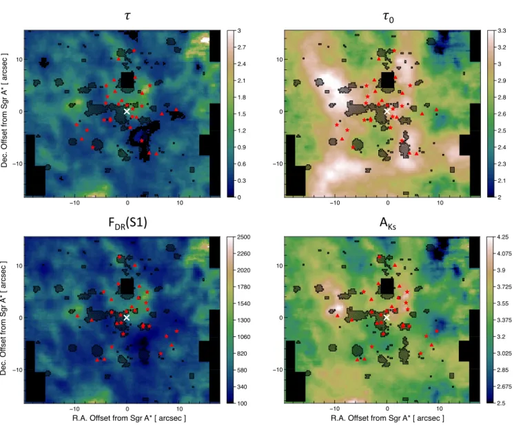
Once given the flux factor, the result is a value of τ and τ0for
each point of the plot (i.e., each pixel on the 2D plane) as shown in Fig.5(top left and top right, respectively).
The τ map very closely resembles the dereddened flux dis-tribution (Fig.5, left bottom) while τ0seems a smoother version
of the AKs map (Fig.5, right bottom). This outcome is
reason-able since τ is supposed to represent the extinction within the emitting shell and is thus naturally correlated with flux in this picture. The fact that the model reproduces the observed correla-tion between the dereddened flux and the extinccorrela-tion rather well strengthens this interpretation.
4.1. Foreground extinction
Assuming that this interpretation is correct, the offset between the distinct curves in Fig.2 (top) corresponds to different fore-ground screen optical thicknesses (i.e., different τ0) for the
various colored areas of Fig.2(bottom).
The differences in screen depth can be interpreted as the geo-metrical location (along the z-axis) of the emitting medium. For a uniform screen, the further away an object is from the observer, the thicker the screen (i.e., higher values of τ0). Indeed, in Fig.2
(bottom), the north-western corner of the observed field corre-sponds to the north-eastern border of the CND. According to the known CND inclination (Liszt 2003), in the observed field, this is the closest portion of the CND to the observer. Consistently, this area corresponds to the lowest foreground extinction among the correlation curves (Fig.2 top, the red curve). On the con-trary, the highest τ0region (magenta and green) encompasses the
Northern Arm of the Minispiral, which is believed to be located at greater line-of-sight distances (Paumard et al. 2004). In this interpretation, the variation of τ0 is foreground relative to the
emitter, but still local to the Galactic center. If this interpretation is correct (further corresponds to more absorbed), then it is only very locally that this extinction is effective since these are indeed very small distance variations when compared to the distance of the Galactic center. On a range of 5-pc scale, δAK=1 translates
to AV ' 2 per parsec. This value, compared to AV =2 for 1 kpc on average through the Galactic disk, is a factor of 1000 larger. This is a big difference, but is not unrealistic: for instance, a Bok globule is very absorbing but also very compact (e.g., inAlves et al. 2001, AV =30 for a diameter of 0.12 pc). Therefore, the
above interpretation is plausible.
However, given the filamentary nature of the ISM, some structure in the foreground extinction is expected and it may account for the observed spatial variations in the screen absorption. For instance, some of the foreground extinction could happen in the clumps and filaments of the central molecular zone (CMZ, Morris & Serabyn 1996). The 20 and 50 km s−1clouds lie very close to the central parsec in projection
(Guesten & Henkel 1983), within 20 pc of SgrA* according to
Molinari et al. (2011) andHenshaw et al.(2016). Therefore, it appears reasonable that CMZ’s material may cause variation of the foreground screen extinction.
4.2. Local extinction
In our model, the flux increases with increasing local extinction because as the physical depth increases the column density of emitting gas increases. However, the increase in flux saturates
D e c. O ff se t fro m Sg r A* [ a rcse c ] D e c. O ff se t fro m Sg r A* [ a rcse c ] −10 0 10 −10 0 10 0 0.3 0.6 0.9 1.2 1.5 1.8 2.1 2.4 2.7 3 −10 0 10 −10 0 10 2 2.1 2.3 2.4 2.5 2.6 2.8 2.9 3 3.2 3.3 −10 0 10 −10 0 10 2.5 2.675 2.85 3.025 3.2 3.375 3.55 3.725 3.9 4.075 4.25 −10 0 10 −10 0 10 100 340 580 820 1060 1300 1540 1780 2020 2260 2500
R.A. Offset from Sgr A* [ arcsec ]
F
DR(S1)
A
Ks𝜏
𝜏
0R.A. Offset from Sgr A* [ arcsec ]
Fig. 5.Top panels: 2D representation of τ (local extinction; left panel) and τ0(screen extinction; right panel) obtained through the simplified
model. These maps closely resemble the dereddened flux (bottom left panel) map and AKsmap (bottom right panel), respectively (bottom images
are fromCiurlo et al. 2016).
when the clump becomes optically thick to exciting UV radi-ation. To make the optical depth variable, so as to sweep the complete curve of correlation, there are two possible scenarios (see Fig.6):
A: Clumps optically thick to IR H2emission: each clump
is irradiated differently and therefore each emitting shell has a different optical depth (τ) in the H2 line. For increasing
opti-cal depth, both emission and extinction are enhanced with the mechanism described in Sect.3. In this scenario only the most external clumps nearest to the observer can be observed (those not hidden behind other clumps). For a photon-dominated region (PDR) in standard conditions, simulations show that the excited H2 is confined to a very thin shell with rshell/Rclump= 1/100–
1/1000 (J. Le Bourlot, priv. comm., see alsoCiurlo et al. 2016). To reproduce Fig.4, the optical depth of this emitting shell has to be on the order of 0.5–1. This interpretation implies that the optical depth of the whole clump is very high (AV= 200–10 000).
This is possible only for very dense clumps.Christopher et al.
(2005) andSmith & Wardle(2014) have shown that such a high
density is reached in many clumps composing the CND.Mills
et al.(2013) finds lower column densities for the CND clumps (∼105–106.5 cm−3). Therefore, for the CND we considered the
clump densities to be in the range 105–107cm−3and the typical
clump size to be of 0.2 pc (Christopher et al. 2005). From nH2/AV = 1.8 × 10²¹ (Predehl & Schmitt 1995) one derives AV= 40–4000. Therefore, the proposed model is compatible
with previous studies.
B: Clumps optically thin to IR H2 emission: for each
clump, the H2emission is produced in a more or less identical
emitting shell of optical depth τ. The H2emission, on its way out
of the medium, is attenuated by bulk dust in other clumps but is also enhanced by the emission coming from the emitting shell of these same clumps. For an increasing number of clumps on the line of sight, both the emission and the extinction are enhanced (see Fig.7). The model is the same as described by Eq. (2), but instead of variable absorption coefficient, we considered n sep-arated, identical clumps. The flux received by the observer is the sum of all contributions of clouds on the line of sight, each one being partially extinguished by those in front of it, plus the foreground screen:
F = [F0+F0e−τC+F0e−2τC+· · · + F0e−(n−1)τC] · e−τ0. (13)
The first term corresponds to the emitting shell closest to the observer (not extinguished by any cloud). The last term
A&A 621, A65 (2019)
A)
B)
Fig. 6.Illustrations of the two scenarios for the flux-extinction correla-tion. In both cases, the H2emission arises from the thin external shell of
clumps. In scenario A, these clumps are optically thick to H2emission
and the emitting shells have variable optical depth (τ1, τ2, τ3, τ4, τ5). In this case, only the most external clumps are visible (1, 2, 4, 5, but
not 3). In scenario B, the clumps are optically thin and are all identical, with optical depth of the emitting shell τ = τC/100. In this case, the
emission coming from a background clump is still visible, provided that there are not too many clumps on the line of sight.
corresponds to the most distant shell, which is suffering extinc-tion from all n − 1 clouds between it and the observer.
Since we assume that the H2 emission is confined in an
external shell of thickness typically 1/100 of the size of the cloud τ = τC/100, and F0 ∝ (1 − e−τC/100), so that we
have
F ∝ (1 − e−τC/100)[1 + e−2τC +· · · + e−(n−1)τC] · e−τ0. (14) We consider τCclose to 1 (which is much less than in hypothesis
A, where τCwas 50–100), so in practice:
F ∝100 ·τC [1 + e−2τC +· · · + e−(n−1)τC] · e−τ0. (15) The final model that best reproduces the observations is the one with from 1 to 20 clumps on the line of sight, each of τC≈ 0.5.
This model works provided that the filling factor by clumps is not too high, allowing a statistically large variation of the num-ber of clumps from one line of sight to the other. In this case, the photons produced by the different clumps would be atten-uated by factors varying in a large range. This scenario would be favored for the central cavity since, there, the filling factor is likely lower than for the CND and the lower medium densities allow for optically thin clumps.
Both scenarios reproduce well the observed slope in the cor-relation plot. Scenario A seems more applicable to the CND if we consider the very high densities derived bySmith & Wardle
(2014), Mills et al. (2013), and Christopher et al. (2005). On the other hand, in the central cavity, a high density cannot be attained. There, scenario B seems to be more appropriate even though it still implies fairly high density (20 clumps of AK ∼ 1 are needed to reproduce the observed dynamics, i.e.,
AKcloud ∼ 20). In practice, the two scenarios probably can
coex-ist in some areas and the final result is likely a superposition of the two effects.
AKs log10 (F) τC τ0 3 3.5 4 2 5 20 n
is short-lived in this highly ionized environment, a small amount can continuously be produced at the surface of dust grains that are present everywhere. The presence of very
Fig. 7. Models from scenario B for different values of the clump absorption coefficient τCand different foreground screen depths: τ0= 3
(black), 3.5 (blue), 4 (red). The variation of τChas the effect of
expand-ing the dynamic range covered by the model. The variation of τ0
shifts the curve to higher extinction values. For τ0= 4 the model is
traced for 20 (black), 5 (red), and 2 (green) clumps with τC= 0.5 each.
Models overlap on the plot and, in fact, all start from the same value. The 20-clump model is the one which covers the whole dynamics. The models reproduce the fact that increasing the number of clumps on the line of sight has the effect of enhancing both the flux and the extinction as observed.
4.3. The global extinction effect
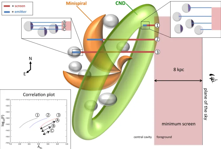
Figure8summarizes our interpretation by showing a schematic representation of the central parsec region, seen from the side.
All emitting shells in the region are subjected to the same 8 kpc Galactic disk extinction. Depending on the distance to the observer and the variation of the ISM along the line of sight, each clump is subject to an additional screen-type extinction. Case 1 in Fig.8corresponds to the curve at the lowest extinction on the correlation plot (red curve in Fig.2). Cases 2 and 3 represent the cases where the screen extinction increases.
As previously mentioned, the clumps of the CND are dense and big, meaning that scenario A (Sect. 4.2) is more repre-sentative: each clump is subject to a different irradiation and shows a different optical depth which is represented by the points along the curve of the correlation plot. In this representation, the medium is continuous.
In the central cavity, the medium is less dense (i.e., has a smaller filling factor), fragmented in smaller-scale clumps, and scenario B (Sect.4.2) is more representative: depending on the number of small clumps on the line of sight the points lay on different parts of the correlation curve (case C in Fig.8shows the lowest number of clumps). A lot of these clumps can over-lap on the line of sight. Given the high number of clumps (20 to cover the whole dynamic range on the correlation plot), scenario B actually reproduces the behavior of a continuous medium.
The two models are therefore not in conflict: they are the extreme representations of two different scale effects. One scenario or the other can apply depending on the scale on which we are observing the ISM. For instance, at the surface of one big clump of scenario A, there could possibly be many much-smaller-scale clumps producing the observed effects, as described in scenario B. We can conclude that, in general, the medium is very clumpy and fragmented.
CND
Minispiral
central cavityminimum screen
8 kpc
= screen = emi1er1
3
2
C AKs log 10 (F) 1 2 A 3 B CCorrela?on plot
plan
e o
f th
e s
ky
foreground B A
N
E
Fig. 8. Representation of the central parsecs along the line of sight. The CND is represented in green, the Minispiral in brown. The clumps of gas and dust in the central cavity are shown in gray. The foreground, purely absorbant “screen” extinction (τ0) is represented in red, the local (τ)
effect of mixed dust and gas (providing for both emission and extinction) is shown in blue. The correlation plot in the bottom-left corner shows the models representing the cases marked on the figure.
5. Conclusions
In Ciurlo et al. (2016), for the first time, the Galactic center extinction map was computed directly from the comparison of two molecular lines: H21-0 S(1) and 1-0 Q(3). Here, we take a
step further by interpreting the results in terms of separate effect of the foreground and local extinction. The computed extinc-tion appears to be correlated locally with the flux map in several distinct regions. Each of these regions is identified by the same slope in the correlation plot.
We propose two models that successfully reproduce the observed correlation. In both models, the correlation is due to the fact that the local emitting H2 is mixed everywhere with
dust. With the help of a simple toy model of radiative trans-fer in a clumpy medium, we showed that in the central parsec around the Galactic center the extinction can be interpreted as a combination of
1. the effect of a purely absorbing, foreground screen and 2. the variation of the optical depth of clumps on the line of
sight (both because of differences in the optical depth and in the number of emitting shells).
Effect (1) causes, for different optical depths of the (purely) absorbing screen, the splitting into multiple curves in the cor-relation plot. Effect (2) causes the variation of the optical depth along the line of sight, and consequently the correlation between the flux and the extinction. In summary, in the correlation plot,
the observed slope traces the fragmentation of the ISM. On the other hand, the split into different groups of correlated points translates into variations in the large-scale foreground extinc-tion. The extinction measured through the Q(3)-S(1) ratio is a combination of both effects.
These results underline the importance of estimating the extinction for the specific emitter under study since each source is located at a different optical depth for the observer. Both local and foreground extinction are important to probe: on one side the local structure of the medium, and on the other side the foreground extinction to which our specific emitter is subjected. The central cavity of the CND is far from being empty: diluted and fragmented clumps of excited molecular gas and dust are located there. The question of the origin of this material is not yet clear (as discussed inCiurlo et al. 2016). The presence of dust could allow for local formation of H2, provided that the grains
are not too hot. Even though one can likely imagine that H2 is
short-lived in this highly ionized environment, a small amount can continuously be produced at the surface of dust grains that are present everywhere. The presence of very hot H2is detected
in other HIIregions as well, such as the Crab Nebula (Scoville et al. 1982). Therefore, it is not so surprising to find some at the Galactic center as well, as was also discussed in Ciurlo et al.
(2016).
It must be noted that the observed H2 lines represent only
A&A 621, A65 (2019)
might be more H2that is not hot enough to be detected in these
lines and not dense enough to be detected through other lines (such as HCN).
In summary, the combined study of several NIR H2lines has
allowed us to learn more about the clumpiness of the medium in the central parsec of the Galaxy. This same kind of study can be applied to other regions where H2is hot enough to be detected
to learn about the structure of the ISM.
Acknowledgements. We would like to thank the infrared group at the Max Planck Institute for Extraterrestrial Physics (MPE), who built the SPIFFI instrument, carried out the observations, and provided the data. We also thank the referee for the useful comments, which helped us improve this paper.
References
Alves, J. F., Lada, C. J., & Lada, E. A. 2001,Nature, 409, 159
Becklin, E. E., & Neugebauer, G. 1968,ApJ, 151, 145
Becklin, E. E., Gatley, I., & Werner, M. W. 1982,ApJ, 258, 135
Beckwith, S., Evans, II, N. J., Gatley, I., Gull, G., & Russell, R. W. 1983,ApJ, 264, 152
Christopher, M. H., Scoville, N. Z., Stolovy, S. R., & Yun, M. S. 2005,ApJ, 622, 346
Ciurlo, A., Paumard, T., Rouan, D., & Clénet, Y. 2016,A&A, 594, A113
Eisenhauer, F., Tecza, M., Thatte, N., et al. 2003,The Messenger, 113, 17
Fritz, T. K., Gillessen, S., Dodds-Eden, K., et al. 2011,ApJ, 737, 73
Gao, J., Li, A., & Jiang, B. W. 2013,Earth Planets Space, 65, 1127
Gautier, III, T. N., Fink, U., Larson, H. P., & Treffers, R. R. 1976,ApJ, 207, L129
Guesten, R., & Henkel, C. 1983,A&A, 125, 136
Henshaw, J. D., Longmore, S. N., Kruijssen, J. M. D., et al. 2016,MNRAS, 457, 2675
Liszt, H. S. 2003,A&A, 408, 1009
Lo, K. Y., & Claussen, M. J. 1983,Nature, 306, 647
Lynden-Bell, D., & Rees, M. J. 1971,MNRAS, 152, 461
Martins, F., Genzel, R., Eisenhauer, F., et al. 2007,Highlights Astron., 14, 207
Mills, E. A. C., Güsten, R., Requena-Torres, M. A., & Morris, M. R. 2013,ApJ, 779, 47
Molinari, S., Bally, J., Noriega-Crespo, A., et al. 2011,ApJ, 735, L33
Morris, M., & Serabyn, E. 1996,ARA&A, 34, 645
Paumard, T., Maillard, J.-P., & Morris, M. 2004,A&A, 426, 81
Paumard, T., Genzel, R., Martins, F., et al. 2006,J. Phys. Conf. Ser., 54, 199
Predehl, P., & Schmitt, J. H. M. M. 1995,A&A, 293, 889
Press, W. H., Teukolsky, S. A., Vetterling, W. T., & Flannery, B. P. 1992,
Numerical Recipes in C. The Art of Scientific Computing (Cambrige: University Press)
Rieke, G. H., Rieke, M. J., & Paul, A. E. 1989,ApJ, 336, 752
Schödel, R., Najarro, F., Muzic, K., & Eckart, A. 2010,A&A, 511, A18
Scoville, N. Z., Hall, D. N. B., Ridgway, S. T., & Kleinmann, S. G. 1982,ApJ, 253, 136
Scoville, N. Z., Stolovy, S. R., Rieke, M., Christopher, M., & Yusef-Zadeh, F. 2003,ApJ, 594, 294
Smith, I. L., & Wardle, M. 2014,MNRAS, 437, 3159
Tecza, M., Thatte, N., Eisenhauer, F., et al. 2000, Optical and IR Telescope Instrumentation and Detectors, SPIE Conf. Ser., 4008, 1344
Appendix A: Estimation of the line absorption coefficient in radiative excitation
For a transition from the upper (i) to the lower ( j) level, the absorption coefficient αjican be calculated as
αji= h νji
4π njBjiφji, (A.1)
where h is the Planck constant, νjiis the line frequency
(here-after ν), and nj the column density (in m−3). The Einstein
coefficient Bjiis given by Bji=Bi jgi gj =Ai j c2 2hν3 gi gj. (A.2)
φjiis the line profile, withR φjidν = 1, and it is given by
φi j= 1 ∆ν= c ν∆v = λi j ∆v, (A.3)
where λi jis the line wavelength and ∆v the line width. One can
therefore write αi j=nj λ3i j 8πAi j gi gj 1 ∆v. (A.4)
The column density can be expressed as nj=nH2· fj, where fj is the relative population of the j-level and is given by
fj= e
−Ej/kT
P e−Ek/kT. (A.5)
For 1-0 S(1) (J = 3 → 1 , v = 1 → 0) at λ = 2.12 µm: Ai j=
3.48 × 10⁻⁷s−1, gi=21, gj=9, and Ej =6.952 × 10³ K. For
a PDR such as the central parsec ∆v ∼ 100 km s−1(Ciurlo et al.
2016), nH2 =105 cm−3(Smith & Wardle 2014) and T = 1200 K as estimated for Orion inBeckwith et al.(1983). Therefore, one finds αi j∼ 2.7 10−22m−1.
Since τi j= αi j· L and a typical clump has a diameter of L =
0.2 pc (Christopher et al. 2005), one finds τi j=1.6 × 10⁻⁶. This
value has to be compared to AV =nH2· L/1.8 1021 (Predehl &
Schmitt 1995). For nH2 =105cm−3it gives τi j/AV =5 × 10⁻⁸ which translates to τi j/AK ∼ 5 × 10⁻⁷. Therefore, the H2 line
is optically thin and there is no self-shielding. The extinction is thus completely due to the dust component of clumps.