HAL Id: hal-00998910
https://hal.archives-ouvertes.fr/hal-00998910
Submitted on 3 Jun 2014
HAL is a multi-disciplinary open access
archive for the deposit and dissemination of
sci-entific research documents, whether they are
pub-lished or not. The documents may come from
teaching and research institutions in France or
abroad, or from public or private research centers.
L’archive ouverte pluridisciplinaire HAL, est
destinée au dépôt et à la diffusion de documents
scientifiques de niveau recherche, publiés ou non,
émanant des établissements d’enseignement et de
recherche français ou étrangers, des laboratoires
publics ou privés.
using linear mixed models with lme R function
Caroline Bazzoli, Frédérique Letué, Marie-José Martinez
To cite this version:
Caroline Bazzoli, Frédérique Letué, Marie-José Martinez. Modelling finger force produced from
dif-ferent tasks using linear mixed models with lme R function. Case Studies in Business, Industry and
Government Statistics, Société Française de Statistique, 2015, 6 (1), pp.16-36. �hal-00998910�
different tasks using linear mixed models
with
❧♠❡ R function
Caroline Bazzoli
Univ. Grenoble Alpes, LJK, F-38000 Grenoble, France
CNRS, LJK, F-38000 Grenoble, France
Frédérique Letué
Univ. Grenoble Alpes, LJK, F-38000 Grenoble, France
CNRS, LJK, F-38000 Grenoble, France
Marie-José Martinez
Univ. Grenoble Alpes, LJK, F-38000 Grenoble, France
CNRS, LJK, F-38000 Grenoble, France
Inria
May 27, 2014
AbstractThe biomechanical data considered in this paper are obtained from a study carried out to understand the coordination patterns of finger forces produced from different tasks. This data cannot be considered independent because of within-individual repeated measurements, and because of simultaneous finger measurements. To fit these data, we propose a methodology focused on linear mixed models. Different random effects structures and complex variance-covariance matrices of the error are considered. We highlight how to use the❧♠❡ R function to deal with such a modelling. The paper is accessible to an audience experienced with linear models. Some familiarity with the R software is also helpful.
Keywords : Linear mixed model, Repeated measures, Heteroscedasticity, Correlation, lme R
function, Biomechanics.
1.
Introduction
In experimental sciences (agronomy, biology, experimental psychology, ...), analysis of vari-ance (ANOVA) is often used to explain one con-tinuous response with respect to different ex-perimental conditions, assuming homoscedas-tic errors. In studies where individuals con-tribute more than one observation, such as lon-gitudinal or repeated-measures studies, classi-cal ANOVA is no longer convenient since the assumption of data independence is not valid. The linear mixed model (Laird and Ware,1982) then provides then a better framework to take correlation between these observations into ac-count. By introducing random effects, mixed models allow to take into account the variabil-ity of the response among the different individ-uals and the possible within-individual corre-lation. Published case studies using a mixed model approach (Baayen et al.,2008;Onyango,
2009) often assume a classical homoscedastic error term, i.e. normally distributed with mean zero and constant variance. In this paper, we consider a case study in which this assumption is relaxed by allowing heteroscedastic and cor-related within-group errors. This work high-lights, in an educationnal way, the different steps of such a modelling.
The data considered in this paper have been ob-tained from a biomechanical study described in detail inQuaine et al.(2012). Experiments have been carried out to better understand the coordination patterns of finger forces produced from different tasks corresponding to different experimental conditions. One of the objectives is to compare each finger force intensity be-tween the various tasks and, for each task, to compare nearby fingers force intensity. Sub-jects are required to press ledges maximally with four fingers simultaneaously in different experimental conditions. Experiments have been repeated three times per experimental condition. InQuaine et al. (2012), data have been analyzed first using a two-factor ANOVA model by considering the force measurement as response and fingers and experimental con-ditions as factors to be tested. Nevertheless, as
pointed out by the authors, in this particular context, the ANOVA model is not convenient since it does not take into account nor the de-pendency between the fingers due to simulta-neous measurements, nor the within-subject dependency due to repeated measurements. There are several facilities in R (R Development Core Team(2008)) and S-PLUS (S-P(1992)) for fitting mixed models to data. Among them are the♥❧♠❡ (Pinheiro et al.,2014) and❧♠❡✹ (Bates et al.,2013) libraries. All analyses in the present paper have been performed using the❧♠❡ func-tion in the♥❧♠❡ library, described in detail in
Pinheiro and Bates(2000). The❧♠❡r function in the❧♠❡✹ library has been developed more recently. This function provides an improve-ment over the ❧♠❡ function, in particular by implementing crossed random effects in a way that is both easier for the user and much faster. However, this function does not offer the same flexibility as the ❧♠❡ function for composing complex variance-covariance structures. In this paper, all analyses have been performed with
the✻✹✲❜✐t ❘ ✈❡rs✐♦♥ ✸✳✶✳✵ ✭✷✵✶✹✲✵✹✲✶✵✮.
The paper is organized as follows. Section 2 presents the data set. Section 3 exposes a pre-liminary study including the basic ANOVA and its limits. Mixed model specification is presented in Section 4, with details on the mod-eling steps. We present and discuss the results in Section 5 and we end with conclusions in Section 6.
2.
The data
The data considered in this paper have been first described in Quaine et al. (2012). Biomechanical researchers propose experi-ments where subjects are submitted to various tasks with the four long fingers (without the thumb). In this study, 15 subjects were required to press ledges maximally with the four fin-gers simultaneously in flexion and extension. First in extension, two force locations at the first (ExtP1) and at the third (ExtP3) phalanx were tested and then in flexion, only the third phalanx location (FlexP3) was tested. From now on, we call❧♦❝❛t✐♦♥ the three
experimen-tal conditions, ExtP3, FlexP3, ExtP1. After 20 trials at low and intermediate intensity, sub-jects are asked to press maximally three times per location, with a one-minute rest to avoid muscular fatigue. Experiments in the three dif-ferent locations were separated by five minute rests.
The data set thus includes 540 measures of finger force intensity (F), subject number (in-dividual from 1 to 15), location (with values ExtP3, FlexP3 and ExtP1), finger (with values I for index, M for middle, R for ring and L for little). For coding purpose, a reiteration vari-able (tr✐❛❧ from 1 to 135) has been added with different numbers from one subject to another and from one location to another. In other words, only 4 simultaneous measures of the four fingers of one reiteration of a given indi-vidual in a given location share the same value of the reiteration variable. The❤❡❛❞ command in R helps to observe the data structure:
❃ ❤❡❛❞✭❉❛t❛✳♥❡✇✱✷✵✵✮ ❋ ❧♦❝❛t✐♦♥ ❢✐♥❣❡r ✐♥❞✐✈ tr✐❛❧ ✶ ✽✳✺✺✶✵✷✺ ❊①tP✸ ■ ✶ ✶ ✷ ✼✳✽✸✻✾✶✹ ❊①tP✸ ■ ✶ ✷ ✸ ✼✳✻✺✸✽✵✾ ❊①tP✸ ■ ✶ ✸ ✹ ✼✳✺✾✽✽✼✼ ❊①tP✸ ■ ✷ ✹ ✺ ✻✳✽✵✺✹✷✵ ❊①tP✸ ■ ✷ ✺ ✻ ✻✳✺✵✻✸✹✽ ❊①tP✸ ■ ✷ ✻ ✳✳✳ ✹✻ ✼✳✺✺✵✵✹✾ ❊①tP✸ ▼ ✶ ✶ ✹✼ ✻✳✽✹✽✶✹✺ ❊①tP✸ ▼ ✶ ✷ ✹✽ ✻✳✾✹✺✽✵✶ ❊①tP✸ ▼ ✶ ✸ ✹✾ ✹✳✹✸✶✶✺✷ ❊①tP✸ ▼ ✷ ✹ ✺✵ ✹✳✺✷✽✽✵✾ ❊①tP✸ ▼ ✷ ✺ ✺✶ ✹✳✻✾✾✼✵✼ ❊①tP✸ ▼ ✷ ✻ ✳✳✳ ✶✽✶ ✷✷✳✹✺✹✽✸✹ ❋❧❡①P✸ ■ ✶ ✹✻ ✶✽✷ ✷✺✳✵✼✾✸✹✻ ❋❧❡①P✸ ■ ✶ ✹✼ ✶✽✸ ✷✷✳✵✵✸✶✼✹ ❋❧❡①P✸ ■ ✶ ✹✽ ✶✽✹ ✷✾✳✻✸✷✺✻✽ ❋❧❡①P✸ ■ ✷ ✹✾ ✶✽✺ ✸✹✳✶✹✸✵✻✻ ❋❧❡①P✸ ■ ✷ ✺✵ ✶✽✻ ✸✹✳✵✺✶✺✶✹ ❋❧❡①P✸ ■ ✷ ✺✶ ✳✳✳
3.
Preliminary study
3.1. Exploratory data analysis
The raw data set is shown in Figure1. One can see that the intensities are clearly higher in FlexP3
lo-cation than in ExtP1 lolo-cation and in ExtP3 lolo-cation, in position but also in scattering. Index measures (blue circles) are nearly always higher than middle measures (red triangles), themselves higher than ring measures (green plus), themselves higher than little measures (magenta times), except in the ExtP1 location where this order appears less often. Dif-ferences between subjects are also to be observed. For instance, individual 4 always has low measures whatever the location, whereas individual 7 always has high measures. One can also see that index and middle measures on the one hand, and ring and little measures on the other hand, are close. This is confirmed by the correlation between fingers illustrated in Figure2.
This exploratory data analysis suggests that inten-sity measures are different from a location to an-other, from a finger to anan-other, but also that a sub-ject effect has to be taken into account. Moreover, simultaneous finger measurements imposed by the experimental design cannot be considered as inde-pendent.
3.2. Two-factor ANOVA and its limits
As already done inQuaine et al.(2012), and even though it is not convenient in this context since we omit the subject effect and the dependence between simultaneous finger measurements, we begin our study with a two-factor ANOVA, namely the loca-tion and the finger effects. In other words, the study is done as if measurements had been done finger by finger, and with 45 different subjects. Following R conventions, our model is thus:
Fl f i =µ+αl+βf+γl f+εl f i (1)
where
• Fl f i is the measurement of
individ-ual i ∈ {1, . . . , 45}, in location l ∈ {ExtP3, FlexP3, ExtP1} and finger f ∈ {I, M, R, L}
• µ is the population measurement of index in location ExtP3
• αlis the overall difference between
measure-ments in location ExtP3 and location l for index (αExtP3=0)
• βf is the overall difference between
measure-ments of index and finger f in location ExtP3 (βI =0)
• γl f is the interaction term of location l and
finger f (γExtP3, f =γl,I=0 )
• εl f i is the residual error, supposed to be
Moreover, all residual errors are supposed to be independent.
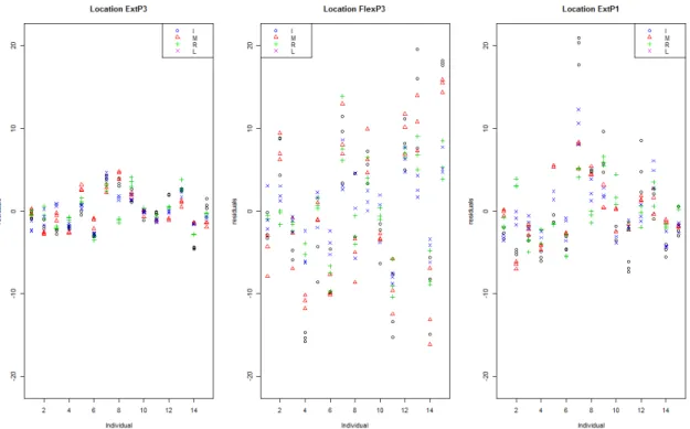
Residuals of the model appear in Figure3. They suffer from several defects:
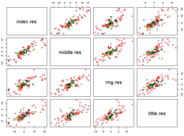
• They are clearly not identically scattered from one location to another, whereas ANOVA model imposes equal variances in all groups. • Some subjects have either all positive or all negative residuals, which suggests a subject effect that has not yet been taken into account. • Residuals still remain very correlated from a finger to another, as it can be seen in Figure4. To deal with these defects, in Section 4, we focus on linear mixed-effects models to fit the data set.
4.
Model specification using a linear
mixed-effects model
4.1. Modelling the random effect structure
Let denote Fl f ik the force measured on finger f
of individual i at trial k in location l with l =
ExtP3, FlexP3, ExtP1, f = I, M, R, L, i = 1, . . . , 15 and k=1, 2, 3. The linear mixed model M0for the
response Fl f ikis defined as
Fl f ik=µ+αl+βf+γl, f+ξi+εl f ik (2)
with αExtP3=0, βI =0, γExtP3, f =γl,I =0. In this
model, µ is the mean for location ExtP3 and finger index, αlis the fixed effect of location l with respect
to location ExtP3, βf is the fixed effect of finger f
with respect to finger index and γl, f is the
interac-tion between locainterac-tion l and finger f . The random effect ξiin (2) is the individual random effect. The
linear mixed model (2) can be rewritten as Fl Iik FlMik FlRik FlLik = µ 1 1 1 1 +αl 1 1 1 1 + βI βM βR βL + γl I γlM γlR γL +ξi 1 1 1 1 + εl Iik εlMik εlRik εlLik (3)
with ξi∼ N (0, τ12)and εlik=
εl Iik εlMik εlRik εlLik ∼ N (0, σ2I)
with I the identity matrix. All random effects are assumed independent from each other and indepen-dent from the error term. Note that the assumption
Var(εlik) =σ2I can be relaxed as shown in section
4.2in order to model unequal variances and specific within-group correlation structures. In the sequel, we use the❧♠❡ function of the ♥❧♠❡ package to fit models. We use the maximum likelihood estima-tion criterion by specifying♠❡t❤♦❞❂✑▼▲✑ in order to compare several models using the❛♥♦✈❛ function. Model M0 is fitted using the R code displayed in
Table1. Figures5and6show that for each location and for each finger, the boxplots of the standard-ized residuals by individual for model M0are not
centred at zero. This clearly suggests that there are different individual effects from one location to another and from one finger to another.
To solve this problem, we introduce a location within individual random effect ξil, a finger within
indi-vidual random effect ξi f and an interaction random
effect between location and finger ξil f leading to
model M1: Fl Iik FlMik FlRik FlLik = µ 1 1 1 1 +αl 1 1 1 1 + βI βM βR βL + γl I γlM γlR γL +ξi 1 1 1 1 +ξil 1 1 1 1 + ξiI ξiM ξiR ξiL + ξil I ξilM ξilR ξilL + εl Iik εlMik εlRik εlLik (4) with ξi ∼ N (0, τ12), ξil ∼ N (0, τ22), ξi f ∼ N (0, τ32), ξil f ∼ N (0, τ42)and εlik= εl Iik εlMik εlRik εlLik ∼ N (0, σ2I). We fit model M1using the R code displayed in Table
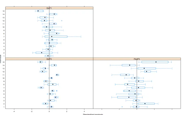
2. For each location and for each finger, the boxplots of the standardized residuals (Figures7and8) by individual for model M1 are now centred at zero.
However, Figure7also indicates that the residual variability is different from a location to another. To take this variability into account, we define a new model M2assuming a different variance per
loca-tion for ξili.e ξil∼ N (0, τl2). This model is fitted in
R using the code displayed in Table3. To compare these models, we first use the ANOVA function as displayed in Table4. The AIC and BIC values and the p-value of the likelihood ratio statistic show that model M2gives a better fit. However, note that this
still remains different residual variability from one location to another.
To deal with this problem, a more general model will be considered in Subsection4.2.1keeping the ran-dom effects structure defined in model M2, but
al-lowing different variances by location for the within-group errors. Moreover, by plotting the pairwise scatter plots of model M2residuals by each pair of
fingers in Figure9, we note that introducing random effect terms in the model did reduce correlations be-tween fingers. Therefore, in Subsection4.2.2, we will consider different correlation structures for the within-group errors.
4.2. Modelling the residual variance-covariance struc-ture
The linear mixed model defined in Section4.1 al-lows flexibility in the specification of the random effects structure, but restricts the within-group er-rors to be independent, identically distributed with mean zero and constant variance. As observed pre-viously, we need to relax this assumption by al-lowing heteroscedastic and correlated within-group errors. Thus, we extend model M2 by assuming
εlik= εl Iik εlMik εlRik εlLik ∼ N (0, σ2Λ
l). Note that the
within-group errors εlikare assumed to be independent for different l , for different i and different k and inde-pendent of the random effects. The 4×4 matrices Λl, l = ExtP3, FlexP3, ExtP1 can be decomposed into a product of simpler matrices Λl = VlClVl,
where Vl is a diagonal matrix containing the
stan-dard deviation of each finger in location l and Cl
is a positive-definite matrix with all diagonal ele-ments equal to 1 describing the correlation of the random vector εlik. This decomposition of Λlinto
a variance structure component and a correlation structure component is convenient both theoretically and computationally. It allows us to model sepa-rately the two structures and to combine them into a flexible family of models. More detail on variance-covariance structures can be found inPinheiro and Bates(2000).
The♥❧♠❡ library provides a set of classes of variance functions, the✈❛r❋✉♥❝ classes, which are used to specify within-group variance structures. The♥❧♠❡ library also provides a set of classes of correlation structures, the❝♦r❙tr✉❝t classes, which are used to model dependence among the within-group er-rors in the context of linear mixed effects models
(Pinheiro and Bates(2000)).
4.2.1 Modelling the variance matrix Vl for
each location
In this subsection, several variance structures Vlare
tested to model residuals. As already pointed out in Section4.1, the variance of residuals clearly differs from one location to another. We therefore consider a first model derived from model M2, noted model
M2.1, assuming a different variance from one
loca-tion to another Vl= σl 0 0 0 0 σl 0 0 0 0 σl 0 0 0 0 σl , Cl = 1 0 0 0 0 1 0 0 0 0 1 0 0 0 0 1 .
Note that, in this model, the correlation matrix Cl,
equal to the identity matrix, assumes no correla-tion between fingers. To fit model M2.1, we use the
✇❡✐❣❤ts argument of the ❧♠❡ function (see Table5). The option❝♦♥tr♦❧❂❧♠❡❈♦♥tr♦❧✭♠s▼❛①■t❡r❂✶✵✵✵✮ makes it possible to increase the maximum number of iterations of the algorithm to achieve convergence. We compare model M2.1 to model M2 using the
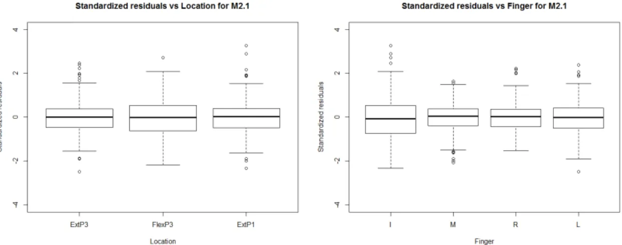
❛♥♦✈❛ function (Table6). The p-value of the likeli-hood ratio statistic shows that the former best fits the data. Figures10and11display boxplots of the standardized residuals by location and by finger from models M2and M2.1 respectively. Note that,
because of different variances by location in model
M2.1, the standardized residuals, displayed in
Fig-ure11, are calculated as the differences between the data Fl f ikand the fitted values ˆFl f ikdivided by the
estimated standard deviation ˆσl.
Figure11shows that, in comparison to model M2,
the standardized residuals are now similarly scat-tered from one location to another. It means that we successfully captured the location variability of the data. However, the index finger variability appears to be different from that of the other fingers. Thus, we introduce model M2.2 by assuming a different
residual variance for the index in each location (de-noted σ2
l I for the index and σlo2 for the other fingers):
Vl= σl I 0 0 0 0 σlo 0 0 0 0 σlo 0 0 0 0 σlo , Cl = 1 0 0 0 0 1 0 0 0 0 1 0 0 0 0 1 .
Figure 12shows that finger variabilities are now similar. Finally, the empirical correlations of the standardized residuals between fingers in model
M2.2 are given in Table7. They are lower than in
the previous models but they remain non negligible between index and middle (0.450) and between ring and little (0.330).
4.2.2 Modelling the correlation matrixCl
Here, we retain the Vlmatrix defined in model M2.2
and we propose different correlation matrix struc-tures to model finger dependence.
In a first step, we define model M2.3 using the
fol-lowing correlation matrix:
Cl = 1 σMI σRI σLI σMI 1 σRM σLM σRI σRM 1 σLR σLI σLM σLR 1 .
To do that, we use the❝♦rr❡❧❛t✐♦♥ argument of the ❧♠❡ function.
Table 8displays AIC and BIC criteria for models
M2.2and M2.3. Using these criteria to compare both
models, we prefer model M2.3taking into account
the correlation residuals between fingers since it has the lowest AIC and BIC. Our choice is confirmed by Figure13, which displays the boxplots of the normal-ized residuals by location and by finger for Model
M2.3. Note that the normalized residuals are
calcu-lated by multiplying the standardized residuals by the inverse square-root factor of the estimated error correlation matrix ˆCl. However, we can observe in
Table9that the correlations between fingers are not really improved with respect to model M2.2.
Nev-ertheless, we keep model M2.3as our final model
because it gives us an interpretable estimated corre-lation matrix.
To explore further this correlation issue, we also compute residual correlations between fingers, loca-tion by localoca-tion in Table10. It appears that there is a different correlation matrix by location. An improve-ment of the final model would thus be to introduce
Cldefined as: Cl =
1 σMIl σRIl σLIl σMIl 1 σRMl σLMl σRIl σRMl 1 σLRl σLIl σLMl σLRl 1 .
Unfortunately, to the best of our knowledge, the ❝♦rr❡❧❛t✐♦♥ option of the ❧♠❡ function does not allow such a modelling.
5.
Results
For exploration of parameter estimates, we again fit model M2.3 with the REML (restricted maximum
likelihood) method. REML is often preferred to ML estimation because it produces unbiased vari-ance parameter estimates (Patterson and Thompson,
1971).
5.1. Residuals analysis of the final model
To confirm the validation of model M2.3, we use the
classical plots (Figure14) for diagnostics purposes: normalized residuals histogram, normal QQ-plot, normalized residuals versus fitted values plot, nor-malized residuals versus observed values plot. The histogram of the residuals and the normal QQ-plot suggest that the residuals fit the normal distribution reasonably well, except for the extreme tails. The residuals versus fitted values plot and the residuals versus observed values plot do not highlight any residual structure.
5.2. Results analysis
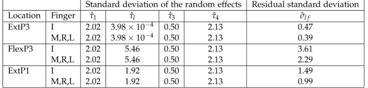
From the❧♠❡ output in Table11, we summarize the REML estimates of the standard deviation compo-nents in Table12. Estimated standard deviations ( ˆτ1, ˆτl, ˆτ2, ˆτ4) of the random effects are directly
ob-tained from the output in the❘❛♥❞♦♠ ❡❢❢❡❝ts part. Moreover, the estimated within-group standard de-viations, ˆσl f, in the last column of Table 12, are
obtained by multiplying the residual term 0.47 by the parameter estimates of the❱❛r✐❛♥❝❡ ❢✉♥❝t✐♦♥ part.
Most variance components have a greater standard deviation than the residual one, hence justifying their inclusion as random effects in the model. The high estimates of the standard deviation compo-nents ˆτ1 and ˆτ4 indicate that the individuals and
the interaction between finger and location clearly contribute to the variability of the data. Concerning the location within individual random effect, an im-portant variability is observed for locations FlexP3 and ExtP1 with ˆτlequal to 5.46 and 1.92 respectively.
Concerning the finger within individual random ef-fect, some variability is also observed, but is lower than the previous ones. Finally, it means that vari-ability of the force measures highly depends on the individual and on the experimental conditions, in particular in flexion at third phalanx location and in extension at first phalanx location.
The❧♠❡ output in Table11also provides estimates of the fixed parameters. The intercept (8.64) is in-terpreted as the average force intensity measure for the index finger in the ExtP3 location. This group of measures is considered as the baseline group and all other groups are compared to this one. For instance, we can see a significant decrease (−2.74) of the force intensity measure for the ring finger in the ExtP3 location compared to the force intensity measure for the index finger in the same location. The aver-age force intensity measure for the former is thus 8.64−2.74=5.90. In the same way, we calculate and display in Table13the estimated mean level of each finger in each location.
In order to provide answers to study objectives, we introduce two contrast analyses. Once the location-finger crossing groups variable (named❣r♦✉♣) is created, we use the❝♦♥str❛sts function of the li-brary▼❆❙❙ (Venables and Ripley,2002), as presented in Table14. Extract of results are displayed in Tables 15and16. We only interpret the lines of the first 8 (resp. 9) groups corresponding to the number of tested contrasts in Table15(resp. Table16) . Table 15shows that, for one given finger, force intensities of each considered pair of locations are significantly different at 5%. On the contrary, one can see in Ta-ble16that the two-by-two finger comparisons show some significant differences:
• In the extension movement, the only significa-tive difference between nearby fingers average force intensities is between the index and the middle on the first phalanx (p-value<1e−06). • In the flexion movement, we notice a signifi-cantly higher average force intensity for the middle than for the ring (p-value<1e−16), and a significantly higher average force in-tensity for the ring than for the little (p-value<1e−11).
The estimation of the correlation matrix between measures of the four fingers is also provided in the ❈♦rr❡❧❛t✐♦♥ s❡❝t✐♦♥ part of the ❧♠❡ output (see Table11). High positive correlations are observed between the measures of index and middle fingers (0.50), ring and little fingers (0.36) and, to a lesser degree, middle and ring fingers (0.22). It means that, in extension and flexion movements, index and mid-dle fingers on the one hand, ring and little fingers on the other hand, seem to vary in the same way.
6.
Conclusion
In this paper, we have proposed a methodology to handle with biomechanical data. The main features of these data lie in the repetition of the force inten-sity measures by individual and the simultaneity of the measures of the four fingers obtained from different tasks. Observations have been fitted using a linear mixed model with a complex random ef-fects structure and a non-diagonal residual variance-covariance matrix using the❧♠❡ R function from the ♥❧♠❡ package. Although some limitations in the implementation of a more complex model have been pointed out, this methodology has been shown to provide the behavior of the force among fingers during different experimental conditions.
The force intensity is different for flexion and ex-tension. In extension, we have found contrasting intensity levels of the index and the middle fingers on the first phalanx. In flexion, we have observed different intensity levels concerning the middle and the ring fingers, as well as concerning the ring and little fingers. Moreover, we have highlighted vari-ous sources of variability for the force intensities, as the individual, the finger and the experimental conditions.
The analysis of the residual correlations in Section 4.2.2fails at giving independent normalized resid-uals, suggesting that a more complex correlation matrix should be introduced. Unfortunately, as far as we know, although the ♥❧♠❡ library provides a large set of classes of correlation structures (the ❝♦r❙tr✉❝t classes), it does not allow such a mod-elling. To deal with this issue, an extension to our work would be to develop a new❝♦r❙tr✉❝t class, integrating a more complex correlation matrix. Thus, the difficulty of dealing with complex data involving the use of linear mixed effects models is clearly illustrated, and the need for further evidence on the implications of this tool is demonstrated.
Acknowledgements
The authors would like to thank Franck Quaine and Florent Paclet for providing access to the data. Collecting the data was financially supported by a PHRC grant (Rhône Alpes). The data analysis has been partially supported by the LabEx PERSYVAL-Lab (ANR-11-LABX-0025-01). The authors thank the PEPS program of the Communauté d’Universités et d’Etablissements Université de Grenoble and CNRS for financial support.
References
(1992). S-PLUS Programmer’s Manual. StatSci, a Divi-sion of MathSoft, Inc., Seattle, WA, USA, verDivi-sion 3.1 edition.
Baayen, R., Davidson, D., and Bates, D. (2008). Mixed-effects modeling with crossed random ef-fects for subjects and items. Journal of Memory and
Language, 59:390–412.
Bates, D., Maechler, M., and Bolker, B. (2013). lme4:
Linear mixed-effects models using S4 classes. R
pack-age version 0.999999-2.
Laird, N. M. and Ware, J. H. (1982). Random-effects models for longitudinal data. Biometrics, 38:963– 974.
Onyango, N. O. (2009). On the linear mixed effects regression (lmer) r function for nested animal breeding data. CSBIGS, 4(1):44–58.
Patterson, H. and Thompson, R. (1971). Recovery of interblock information when block sizes are unequal. Biometrika, 58(3):545–554.
Pinheiro, J. and Bates, D. (2000). Mixed-effects models
in S and S-Plus. Springer-Verlag, New-York.
Pinheiro, J., Bates, D., DebRoy, S., Sarkar, D., and R Core Team (2014). nlme: Linear and Nonlinear
Mixed Effects Models. R package version 3.1-117.
Quaine, F., Paclet, F., Letué, F., and Moutet, F. (2012). Force sharing and neutral line during finger extension tasks. Human Movement Science, 31(4):749–757.
R Development Core Team (2008). R: A Language
and Environment for Statistical Computing. R
Foun-dation for Statistical Computing, Vienna, Austria. ISBN 3-900051-07-0.
Venables, W. N. and Ripley, B. D. (2002). Modern
Ap-plied Statistics with S. Springer, New York, fourth
edition. ISBN 0-387-95457-0.
Tables
Table 1: R code for fitting model M0and plot-ting the residuals
❢✐t▼✵ ❁✲ ❧♠❡✭❋ ⑦ ❢✐♥❣❡r✯❧♦❝❛t✐♦♥✱ r❛♥❞♦♠❂⑦✶⑤✐♥❞✐✈✐❞✉❛❧✱ ♠❡t❤♦❞❂✧▼▲✧✮ s✉♠♠❛r②✭❢✐t▼✵✮
r❡s▼✵✳st❞ ❁✲ r❡s✐❞✉❛❧s✭❢✐t▼✵✱t②♣❡❂✧♣❡❛rs♦♥✧✮
♣❧♦t✭❢✐t▼✵✱✐♥❞✐✈✐❞✉❛❧⑦r❡s▼✵✳st❞⑤❧♦❝❛t✐♦♥✱❛❜❧✐♥❡❂✵✱①❧✐♠❂❝✭✲✺✱✺✮✱①❧❛❜❂✧❙t❛♥❞❛r❞✐③❡❞ r❡s✐❞✉❛❧s✧✮ ♣❧♦t✭❢✐t▼✵✱✐♥❞✐✈✐❞✉❛❧⑦r❡s▼✵✳st❞⑤❢✐♥❣❡r✱❛❜❧✐♥❡❂✵✱①❧✐♠❂❝✭✲✺✱✺✮✱ ①❧❛❜❂✧❙t❛♥❞❛r❞✐③❡❞ r❡s✐❞✉❛❧s✧✮
Table 2: R code for fitting model M1and plot-ting the residuals
❢✐t▼✶ ❁✲ ❧♠❡✭❋ ⑦ ❢✐♥❣❡r✯❧♦❝❛t✐♦♥✱ r❛♥❞♦♠❂❧✐st✭✐♥❞✐✈✐❞✉❛❧❂♣❞❇❧♦❝❦❡❞✭❧✐st✭♣❞■❞❡♥t✭⑦✶✮✱ ♣❞■❞❡♥t✭⑦❧♦❝❛t✐♦♥✲✶✮✱ ♣❞■❞❡♥t✭⑦❢✐♥❣❡r✲✶✮✱ ♣❞■❞❡♥t✭⑦❧♦❝❛t✐♦♥✿❢✐♥❣❡r✲✶✮✮✮✮✱ ♠❡t❤♦❞❂✧▼▲✧✮ r❡s▼✶✳st❞ ❁✲ r❡s✐❞✉❛❧s✭❢✐t▼✶✱t②♣❡❂✧♣❡❛rs♦♥✧✮ ♣❧♦t✭❢✐t▼✶✱✐♥❞✐✈✐❞✉❛❧⑦r❡s▼✶✳st❞⑤❧♦❝❛t✐♦♥✱❛❜❧✐♥❡❂✵✱①❧✐♠❂❝✭✲✺✱✺✮✱ ①❧❛❜❂✧❙t❛♥❞❛r❞✐③❡❞ r❡s✐❞✉❛❧s✧✮ ♣❧♦t✭❢✐t▼✶✱✐♥❞✐✈✐❞✉❛❧⑦r❡s▼✶✳st❞⑤❢✐♥❣❡r✱❛❜❧✐♥❡❂✵✱①❧✐♠❂❝✭✲✺✱✺✮✱ ①❧❛❜❂✧❙t❛♥❞❛r❞✐③❡❞ r❡s✐❞✉❛❧s✧✮
Table 3: R code for fitting model M2
❢✐t▼✷ ❁✲ ❧♠❡✭❋ ⑦ ❢✐♥❣❡r✯❧♦❝❛t✐♦♥✱ r❛♥❞♦♠❂❧✐st✭✐♥❞✐✈✐❞✉❛❧❂♣❞❇❧♦❝❦❡❞✭❧✐st✭♣❞■❞❡♥t✭⑦✶✮✱ ♣❞❉✐❛❣✭⑦❧♦❝❛t✐♦♥✲✶✮✱ ♣❞■❞❡♥t✭⑦❢✐♥❣❡r✲✶✮✱ ♣❞■❞❡♥t✭⑦❧♦❝❛t✐♦♥✿❢✐♥❣❡r✲✶✮✮✮✮✱ ♠❡t❤♦❞❂✧▼▲✧✮
Table 4: R code for comparing models M0, M1 and M2 ❃ ❛♥♦✈❛✭❢✐t▼✵✱❢✐t▼✶✱❢✐t▼✷✮ ▼♦❞❡❧ ❞❢ ❆■❈ ❇■❈ ❧♦❣▲✐❦ ❚❡st ▲✳❘❛t✐♦ ♣✲✈❛❧✉❡ ❢✐t▼✵ ✶ ✶✹ ✸✵✻✷✳✻✶✹ ✸✶✷✷✳✻✾✻ ✲✶✺✶✼✳✸✵✼ ❢✐t▼✶ ✷ ✶✼ ✷✺✺✾✳✺✺✹ ✷✻✸✷✳✺✶✶ ✲✶✷✻✷✳✼✼✼ ✶ ✈s ✷ ✺✵✾✳✵✻✵✸ ❁✳✵✵✵✶ ❢✐t▼✷ ✸ ✶✾ ✷✺✸✻✳✻✷✸ ✷✻✶✽✳✶✻✸ ✲✶✷✹✾✳✸✶✷ ✷ ✈s ✸ ✷✻✳✾✸✶✵ ❁✳✵✵✵✶
Table 5: R code for fitting model M2.1 ❢✐t▼✷✳✶ ❁✲ ❧♠❡✭❋ ⑦ ❢✐♥❣❡r✯❧♦❝❛t✐♦♥✱ r❛♥❞♦♠❂❧✐st✭✐♥❞✐✈✐❞✉❛❧❂♣❞❇❧♦❝❦❡❞✭❧✐st✭♣❞■❞❡♥t✭⑦✶✮✱ ♣❞❉✐❛❣✭⑦❧♦❝❛t✐♦♥✲✶✮✱ ♣❞■❞❡♥t✭⑦❢✐♥❣❡r✲✶✮✱ ♣❞■❞❡♥t✭⑦❧♦❝❛t✐♦♥✿❢✐♥❣❡r✲✶✮✮✮✮✱ ✇❡✐❣❤ts❂✈❛r■❞❡♥t✭❢♦r♠❂⑦✶⑤❧♦❝❛t✐♦♥✮✱ ♠❡t❤♦❞❂✧▼▲✧✱❝♦♥tr♦❧❂❧♠❡❈♦♥tr♦❧✭♠s▼❛①■t❡r❂✶✵✵✵✮✮
Table 6:R code for comparing models M2and
M2.1.
❃ ❛♥♦✈❛✭❢✐t▼✷✱❢✐t▼✷✳✶✮
▼♦❞❡❧ ❞❢ ❆■❈ ❇■❈ ❧♦❣▲✐❦ ❚❡st ▲✳❘❛t✐♦ ♣✲✈❛❧✉❡
❢✐t▼✷ ✶ ✶✾ ✷✺✸✻✳✻✷✸ ✷✻✶✽✳✶✻✸ ✲✶✷✹✾✳✸✶✷
❢✐t▼✷✳✶ ✷ ✷✶ ✷✷✵✾✳✹✺✵ ✷✷✾✾✳✺✼✸ ✲✶✵✽✸✳✼✷✺ ✶ ✈s ✷ ✸✸✶✳✶✼✸✸ ❁✳✵✵✵✶
Table 7: Correlation between finger residuals from model M2.2 ✐♥❞❡①✳r❡s▼✷✳✷✳st❞ ♠✐❞❞❧❡✳r❡s▼✷✳✷✳st❞ r✐♥❣✳r❡s▼✷✳✷✳st❞ ❧✐tt❧❡✳r❡s▼✷✳✷✳st❞ ✐♥❞❡①✳r❡s▼✷✳✷✳st❞ ✶✳✵✵✵✵✵✵✵✵✵ ✵✳✹✹✾✾✸✹✷✾ ✵✳✵✺✷✽✺✽✵✽ ✵✳✵✵✷✽✽✵✵✷✶ ♠✐❞❞❧❡✳r❡s▼✷✳✷✳st❞ ✵✳✹✹✾✾✸✹✷✾✶ ✶✳✵✵✵✵✵✵✵✵ ✵✳✶✾✼✽✼✺✶✺ ✲✵✳✵✺✹✷✼✸✺✻✵ r✐♥❣✳r❡s▼✷✳✷✳st❞ ✵✳✵✺✷✽✺✽✵✽✸ ✵✳✶✾✼✽✼✺✶✺ ✶✳✵✵✵✵✵✵✵✵ ✵✳✸✸✵✵✹✵✸✼✺ ❧✐tt❧❡✳r❡s▼✷✳✷✳st❞ ✵✳✵✵✷✽✽✵✵✷✶ ✲✵✳✵✺✹✷✼✸✺✻ ✵✳✸✸✵✵✹✵✸✼ ✶✳✵✵✵✵✵✵✵✵✵
Table 8: R code for comparing models M2.2 and M2.3.
❃ ❛♥♦✈❛✭❢✐t▼✷✳✷✱ ❢✐t▼✷✳✸✮
▼♦❞❡❧ ❞❢ ❆■❈ ❇■❈ ❧♦❣▲✐❦ ❚❡st ▲✳❘❛t✐♦ ♣✲✈❛❧✉❡
❢✐t▼✷✳✷ ✶ ✷✹ ✷✶✾✻✳✶✽✶ ✷✷✾✾✳✶✼✽ ✲✶✵✼✹✳✵✾✵
❢✐t▼✷✳✸ ✷ ✸✵ ✷✶✻✸✳✾✽✹ ✷✷✾✷✳✼✸✶ ✲✶✵✺✶✳✾✾✷ ✶ ✈s ✷ ✹✹✳✶✾✻✺✼ ❁✳✵✵✵✶
Table 9: Correlation between finger residuals from model M2.3 ✐♥❞❡①✳r❡s▼✷✳✸✳♥♦r♠ ♠✐❞❞❧❡✳r❡s▼✷✳✸✳♥♦r♠ r✐♥❣✳r❡s▼✷✳✸✳♥♦r♠ ❧✐tt❧❡✳r❡s▼✷✳✸✳♥♦r♠ ✐♥❞❡①✳r❡s▼✷✳✸✳♥♦r♠ ✶✳✵✵✵✵✵✵✵✵✵✵ ✵✳✹✸✹✾✺✼✼ ✵✳✵✼✻✾✵✼✺✹ ✲✵✳✵✵✵✾✹✹✻✺✶✾ ♠✐❞❞❧❡✳r❡s▼✷✳✸✳♥♦r♠ ✵✳✹✸✹✾✺✼✻✾✻✹ ✶✳✵✵✵✵✵✵✵ ✵✳✶✽✻✻✶✹✶✾ ✲✵✳✶✵✵✵✹✵✷✺✷✶ r✐♥❣✳r❡s▼✷✳✸✳♥♦r♠ ✵✳✵✼✻✾✵✼✺✹✸✺ ✵✳✶✽✻✻✶✹✷ ✶✳✵✵✵✵✵✵✵✵ ✵✳✸✶✻✵✶✵✷✸✻✺ ❧✐tt❧❡✳r❡s▼✷✳✸✳♥♦r♠ ✲✵✳✵✵✵✾✹✹✻✺✶✾ ✲✵✳✶✵✵✵✹✵✸ ✵✳✸✶✻✵✶✵✷✹ ✶✳✵✵✵✵✵✵✵✵✵✵
Table 10: Correlation between finger residuals from model M2.3 ❬✶❪ ✧❊①tP✸✧ ✐♥❞❡①✳❊①tP✸ ♠✐❞❞❧❡✳❊①tP✸ r✐♥❣✳❊①tP✸ ❧✐tt❧❡✳❊①tP✸ ✐♥❞❡①✳❊①tP✸ ✶✳✵✵✵✵✵✵✵✵ ✵✳✷✾✼✵✸✶✵✽ ✵✳✵✶✺✻✼✵✽✻ ✵✳✶✶✺✽✾✹✼✻ ♠✐❞❞❧❡✳❊①tP✸ ✵✳✷✾✼✵✸✶✵✽ ✶✳✵✵✵✵✵✵✵✵ ✵✳✶✷✸✼✾✵✷✾ ✵✳✵✹✹✺✻✸✷✽ r✐♥❣✳❊①tP✸ ✵✳✵✶✺✻✼✵✽✻ ✵✳✶✷✸✼✾✵✷✾ ✶✳✵✵✵✵✵✵✵✵ ✵✳✹✹✾✼✵✼✷✻ ❧✐tt❧❡✳❊①tP✸ ✵✳✶✶✺✽✾✹✼✻ ✵✳✵✹✹✺✻✸✷✽ ✵✳✹✹✾✼✵✼✷✻ ✶✳✵✵✵✵✵✵✵✵ ❬✶❪ ✧❋❧❡①P✸✧ ✐♥❞❡①✳❋❧❡①P✸ ♠✐❞❞❧❡✳❋❧❡①P✸ r✐♥❣✳❋❧❡①P✸ ❧✐tt❧❡✳❋❧❡①P✸ ✐♥❞❡①✳❋❧❡①P✸ ✶✳✵✵✵✵✵✵✵✵ ✵✳✺✵✷✵✶✹✽ ✵✳✵✽✶✺✾✾✻✹ ✲✵✳✶✼✶✵✹✸✼ ♠✐❞❞❧❡✳❋❧❡①P✸ ✵✳✺✵✷✵✶✹✼✾ ✶✳✵✵✵✵✵✵✵ ✵✳✸✷✺✾✻✹✶✷ ✲✵✳✶✹✵✺✽✺✹ r✐♥❣✳❋❧❡①P✸ ✵✳✵✽✶✺✾✾✻✹ ✵✳✸✷✺✾✻✹✶ ✶✳✵✵✵✵✵✵✵✵ ✵✳✹✷✺✺✾✾✹ ❧✐tt❧❡✳❋❧❡①P✸ ✲✵✳✶✼✶✵✹✸✼✸ ✲✵✳✶✹✵✺✽✺✹ ✵✳✹✷✺✺✾✾✹✵ ✶✳✵✵✵✵✵✵✵ ❬✶❪ ✧❊①tP✶✧ ✐♥❞❡①✳❊①tP✶ ♠✐❞❞❧❡✳❊①tP✶ r✐♥❣✳❊①tP✶ ❧✐tt❧❡✳❊①tP✶ ✐♥❞❡①✳❊①tP✶ ✶✳✵✵✵✵✵✵✵ ✵✳✹✾✷✷✶✵✷ ✵✳✶✷✼✼✹✷✹ ✵✳✵✼✸✶✼✾✻ ♠✐❞❞❧❡✳❊①tP✶ ✵✳✹✾✷✷✶✵✷ ✶✳✵✵✵✵✵✵✵ ✵✳✶✶✻✼✻✷✼ ✲✵✳✶✾✷✷✽✸✸ r✐♥❣✳❊①tP✶ ✵✳✶✷✼✼✹✷✹ ✵✳✶✶✻✼✻✷✼ ✶✳✵✵✵✵✵✵✵ ✵✳✶✷✷✵✼✼✷ ❧✐tt❧❡✳❊①tP✶ ✵✳✵✼✸✶✼✾✻ ✲✵✳✶✾✷✷✽✸✸ ✵✳✶✷✷✵✼✼✷ ✶✳✵✵✵✵✵✵✵
Table 11: Extract from the❧♠❡ output for the final model ▲✐♥❡❛r ♠✐①❡❞✲❡❢❢❡❝ts ♠♦❞❡❧ ❢✐t ❜② ❘❊▼▲ ❉❛t❛✿ ◆❯▲▲ ❆■❈ ❇■❈ ❧♦❣▲✐❦ ✷✶✹✽✳✺✸✼ ✷✷✼✻✳✻✶ ✲✶✵✹✹✳✷✻✽ ❘❛♥❞♦♠ ❡❢❢❡❝ts✿ ❈♦♠♣♦s✐t❡ ❙tr✉❝t✉r❡✿ ❇❧♦❝❦❡❞ ❇❧♦❝❦ ✶✿ ✭■♥t❡r❝❡♣t✮ ❋♦r♠✉❧❛✿ ⑦✶ ⑤ ✐♥❞✐✈✐❞✉❛❧ ✭■♥t❡r❝❡♣t✮ ❙t❞❉❡✈✿ ✷✳✵✶✺✹✽✸ ❇❧♦❝❦ ✷✿ ❧♦❝❛t✐♦♥❊①tP✸✱ ❧♦❝❛t✐♦♥❋❧❡①P✸✱ ❧♦❝❛t✐♦♥❊①tP✶ ❋♦r♠✉❧❛✿ ⑦❧♦❝❛t✐♦♥ ✲ ✶ ⑤ ✐♥❞✐✈✐❞✉❛❧ ❙tr✉❝t✉r❡✿ ❉✐❛❣♦♥❛❧ ❧♦❝❛t✐♦♥❊①tP✸ ❧♦❝❛t✐♦♥❋❧❡①P✸ ❧♦❝❛t✐♦♥❊①tP✶ ❙t❞❉❡✈✿ ✵✳✵✵✵✸✾✼✾✸✵✾ ✺✳✹✻✸✼✼✼ ✶✳✾✷✷✹✺✸ ❇❧♦❝❦ ✸✿ ❢✐♥❣❡r■✱ ❢✐♥❣❡r▼✱ ❢✐♥❣❡r❘✱ ❢✐♥❣❡r▲ ❋♦r♠✉❧❛✿ ⑦❢✐♥❣❡r ✲ ✶ ⑤ ✐♥❞✐✈✐❞✉❛❧ ❙tr✉❝t✉r❡✿ ▼✉❧t✐♣❧❡ ♦❢ ❛♥ ■❞❡♥t✐t② ❢✐♥❣❡r■ ❢✐♥❣❡r▼ ❢✐♥❣❡r❘ ❢✐♥❣❡r▲ ❙t❞❉❡✈✿ ✵✳✹✾✼✶✺✶✾ ✵✳✹✾✼✶✺✶✾ ✵✳✹✾✼✶✺✶✾ ✵✳✹✾✼✶✺✶✾ ❇❧♦❝❦ ✹✿ ❧♦❝❛t✐♦♥❊①tP✸✿❢✐♥❣❡r■✱ ❧♦❝❛t✐♦♥❋❧❡①P✸✿❢✐♥❣❡r■✱ ❧♦❝❛t✐♦♥❊①tP✶✿❢✐♥❣❡r■✱ ❧♦❝❛t✐♦♥❊①tP✸✿❢✐♥❣❡r▼✱ ❧♦❝❛t✐♦♥❋❧❡①P✸✿❢✐♥❣❡r▼✱ ❧♦❝❛t✐♦♥❊①tP✶✿❢✐♥❣❡r▼✱ ❧♦❝❛t✐♦♥❊①tP✸✿❢✐♥❣❡r❘✱ ❧♦❝❛t✐♦♥❋❧❡①P✸✿❢✐♥❣❡r❘✱ ❧♦❝❛t✐♦♥❊①tP✶✿❢✐♥❣❡r❘✱ ❧♦❝❛t✐♦♥❊①tP✸✿❢✐♥❣❡r▲✱ ❧♦❝❛t✐♦♥❋❧❡①P✸✿❢✐♥❣❡r▲✱ ❧♦❝❛t✐♦♥❊①tP✶✿❢✐♥❣❡r▲ ❋♦r♠✉❧❛✿ ⑦❧♦❝❛t✐♦♥✿❢✐♥❣❡r ✲ ✶ ⑤ ✐♥❞✐✈✐❞✉❛❧ ❙tr✉❝t✉r❡✿ ▼✉❧t✐♣❧❡ ♦❢ ❛♥ ■❞❡♥t✐t② ❧♦❝❛t✐♦♥❊①tP✸✿❢✐♥❣❡r■ ❧♦❝❛t✐♦♥❋❧❡①P✸✿❢✐♥❣❡r■ ❧♦❝❛t✐♦♥❊①tP✶✿❢✐♥❣❡r■ ❙t❞❉❡✈✿ ✷✳✶✸✶✾✵✸ ✷✳✶✸✶✾✵✸ ✷✳✶✸✶✾✵✸ ❧♦❝❛t✐♦♥❊①tP✸✿❢✐♥❣❡r▼ ❧♦❝❛t✐♦♥❋❧❡①P✸✿❢✐♥❣❡r▼ ❧♦❝❛t✐♦♥❊①tP✶✿❢✐♥❣❡r▼ ❙t❞❉❡✈✿ ✷✳✶✸✶✾✵✸ ✷✳✶✸✶✾✵✸ ✷✳✶✸✶✾✵✸ ❧♦❝❛t✐♦♥❊①tP✸✿❢✐♥❣❡r❘ ❧♦❝❛t✐♦♥❋❧❡①P✸✿❢✐♥❣❡r❘ ❧♦❝❛t✐♦♥❊①tP✶✿❢✐♥❣❡r❘ ❙t❞❉❡✈✿ ✷✳✶✸✶✾✵✸ ✷✳✶✸✶✾✵✸ ✷✳✶✸✶✾✵✸ ❧♦❝❛t✐♦♥❊①tP✸✿❢✐♥❣❡r▲ ❧♦❝❛t✐♦♥❋❧❡①P✸✿❢✐♥❣❡r▲ ❧♦❝❛t✐♦♥❊①tP✶✿❢✐♥❣❡r▲ ❙t❞❉❡✈✿ ✷✳✶✸✶✾✵✸ ✷✳✶✸✶✾✵✸ ✷✳✶✸✶✾✵✸ ❘❡s✐❞✉❛❧ ❙t❞❉❡✈✿ ✵✳✹✻✼✷✽✸ ❈♦rr❡❧❛t✐♦♥ ❙tr✉❝t✉r❡✿ ●❡♥❡r❛❧ ❋♦r♠✉❧❛✿ ⑦✶ ⑤ ✐♥❞✐✈✐❞✉❛❧✴tr✐❛❧ P❛r❛♠❡t❡r ❡st✐♠❛t❡✭s✮✿ ❈♦rr❡❧❛t✐♦♥✿ ✶ ✷ ✸ ✷ ✵✳✹✾✽ ✸ ✵✳✵✽✷ ✵✳✷✶✼ ✹ ✵✳✵✵✺ ✲✵✳✵✸✾ ✵✳✸✻✵
❱❛r✐❛♥❝❡ ❢✉♥❝t✐♦♥✿ ❙tr✉❝t✉r❡✿ ❉✐❢❢❡r❡♥t st❛♥❞❛r❞ ❞❡✈✐❛t✐♦♥s ♣❡r str❛t✉♠ ❋♦r♠✉❧❛✿ ⑦✶ ⑤ ❧♦❝❛t✐♦♥ ✯ ■♥❞❡① P❛r❛♠❡t❡r ❡st✐♠❛t❡s✿ ❊①tP✸✯■ ❊①tP✸✯♦t❤❡r ❋❧❡①P✸✯■ ❋❧❡①P✸✯♦t❤❡r ❊①tP✶✯■ ❊①tP✶✯♦t❤❡r ✶✳✵✵✵✵✵✵✵ ✵✳✽✸✺✸✶✵✽ ✼✳✼✸✻✻✸✽✻ ✹✳✽✾✺✹✵✼✾ ✸✳✶✾✸✼✶✷✽ ✷✳✶✸✷✾✾✶✽ ❋✐①❡❞ ❡❢❢❡❝ts✿ ❋ ⑦ ❢✐♥❣❡r ✯ ❧♦❝❛t✐♦♥ ❱❛❧✉❡ ❙t❞✳❊rr♦r ❉❋ t✲✈❛❧✉❡ ♣✲✈❛❧✉❡ ✭■♥t❡r❝❡♣t✮ ✽✳✻✹✹✽✽✹ ✵✳✼✼✶✹✺✹✸ ✺✶✹ ✶✶✳✷✵✺✾✺✽ ✵✳✵✵✵✵ ❢✐♥❣❡r▼ ✲✶✳✸✾✸✸✻✺ ✵✳✽✵✶✾✼✸✶ ✺✶✹ ✲✶✳✼✸✼✹✷✶ ✵✳✵✽✷✾ ❢✐♥❣❡r❘ ✲✷✳✼✹✷✷✹✷ ✵✳✽✵✹✵✻✽✹ ✺✶✹ ✲✸✳✹✶✵✹✺✽ ✵✳✵✵✵✼ ❢✐♥❣❡r▲ ✲✸✳✻✼✼✶✻✺ ✵✳✽✵✹✹✺✽✺ ✺✶✹ ✲✹✳✺✼✵✾✽✶ ✵✳✵✵✵✵ ❧♦❝❛t✐♦♥❋❧❡①P✸ ✶✻✳✻✸✷✵✽✵ ✶✳✼✵✵✹✸✺✼ ✺✶✹ ✾✳✼✽✶✵✼✵ ✵✳✵✵✵✵ ❧♦❝❛t✐♦♥❊①tP✶ ✻✳✵✽✹✾✸✹ ✵✳✾✺✷✷✷✻✵ ✺✶✹ ✻✳✸✾✵✷✷✵ ✵✳✵✵✵✵ ❢✐♥❣❡r▼✿❧♦❝❛t✐♦♥❋❧❡①P✸ ✶✳✺✽✺✹✷✷ ✶✳✷✵✵✵✷✺✻ ✺✶✹ ✶✳✸✷✶✶✺✼ ✵✳✶✽✼✵ ❢✐♥❣❡r❘✿❧♦❝❛t✐♦♥❋❧❡①P✸ ✲✺✳✷✾✹✽✻✽ ✶✳✷✻✸✸✸✸✷ ✺✶✹ ✲✹✳✶✾✶✶✽✽ ✵✳✵✵✵✵ ❢✐♥❣❡r▲✿❧♦❝❛t✐♦♥❋❧❡①P✸ ✲✶✵✳✶✷✻✻✽✷ ✶✳✷✼✹✼✽✾✾ ✺✶✹ ✲✼✳✾✹✸✽✵✹ ✵✳✵✵✵✵ ❢✐♥❣❡r▼✿❧♦❝❛t✐♦♥❊①tP✶ ✲✷✳✶✼✹✹✼✾ ✶✳✶✷✵✷✶✻✹ ✺✶✹ ✲✶✳✾✹✶✶✷✹ ✵✳✵✺✷✽ ❢✐♥❣❡r❘✿❧♦❝❛t✐♦♥❊①tP✶ ✲✷✳✶✺✸✼✷✼ ✶✳✶✸✸✽✽✹✼ ✺✶✹ ✲✶✳✽✾✾✹✷✹ ✵✳✵✺✽✶ ❢✐♥❣❡r▲✿❧♦❝❛t✐♦♥❊①tP✶ ✲✵✳✶✵✼✺✺✽ ✶✳✶✸✻✹✶✺✶ ✺✶✹ ✲✵✳✵✾✹✻✹✻ ✵✳✾✷✹✻
Table 12: REML estimates of the standard de-viation components for the final model
Standard deviation of the random effects Residual standard deviation
Location Finger ˆτ1 ˆτl ˆτ3 ˆτ4 ˆσl f ExtP3 I 2.02 3.98
×
10−4 0.50 2.13 0.47 M,R,L 2.02 3.98×
10−4 0.50 2.13 0.39 FlexP3 I 2.02 5.46 0.50 2.13 3.61 M,R,L 2.02 5.46 0.50 2.13 2.29 ExtP1 I 2.02 1.92 0.50 2.13 1.49 M,R,L 2.02 1.92 0.50 2.13 0.99Table 13:Estimated mean levels of the location-finger crossing groups.
Location / finger Index Middle Ring Little
ExtP3 8.64 7.25 5.90 4.97
FlexP3 25.28 25.47 17.24 11.47
Table 14: R code for contrast analysis. ❣r♦✉♣ ❁✲ ❣❧✭✶✷✱✹✺✱✺✹✵✱❧❛❜❡❧s❂❝✭✧❊①tP✸✿■✧✱✧❊①tP✸✿▼✧✱✧❊①tP✸✿❘✧✱✧❊①tP✸✿▲✧✱ ✧❋❧❡①P✸✿■✧✱✧❋❧❡①P✸✿▼✧✱✧❋❧❡①P✸✿❘✧✱✧❋❧❡①P✸✿▲✧✱ ✧❊①tP✶✿■✧✱✧❊①tP✶✿▼✧✱✧❊①tP✶✿❘✧✱✧❊①tP✶✿▲✧✮✮ ❧✐❜r❛r②✭▼❆❙❙✮ ▼✳❧♦❝❛t✐♦♥❁✲❝❜✐♥❞✭ ❝✭✶✱✵✱✵✱✵✱✲✶✱✵✱✵✱✵✱✵✱✵✱✵✱✵✮✱ ★ ❊①tP✸✴❋❧❡①P✸✱■ ❝✭✵✱✶✱✵✱✵✱✵✱✲✶✱✵✱✵✱✵✱✵✱✵✱✵✮✱ ★ ❊①tP✸✴❋❧❡①P✸✱▼ ❝✭✵✱✵✱✶✱✵✱✵✱✵✱✲✶✱✵✱✵✱✵✱✵✱✵✮✱ ★ ❊①tP✸✴❋❧❡①P✸✱❘ ❝✭✵✱✵✱✵✱✶✱✵✱✵✱✵✱✲✶✱✵✱✵✱✵✱✵✮✱ ★ ❊①tP✸✴❋❧❡①P✸✱▲ ❝✭✶✱✵✱✵✱✵✱✵✱✵✱✵✱✵✱✲✶✱✵✱✵✱✵✮✱ ★ ❊①tP✸✴❊①tP✶✱■ ❝✭✵✱✶✱✵✱✵✱✵✱✵✱✵✱✵✱✵✱✲✶✱✵✱✵✮✱ ★ ❊①tP✸✴❊①tP✶✱▼ ❝✭✵✱✵✱✶✱✵✱✵✱✵✱✵✱✵✱✵✱✵✱✲✶✱✵✮✱ ★ ❊①tP✸✴❊①tP✶✱❘ ❝✭✵✱✵✱✵✱✶✱✵✱✵✱✵✱✵✱✵✱✵✱✵✱✲✶✮ ★ ❊①tP✸✴❊①tP✶✱▲ ✮ ❝♦♥tr❛sts✭❣r♦✉♣✮❁✲t✭❣✐♥✈✭▼✳❧♦❝❛t✐♦♥✮✮ ❢✐t▼✷✳✸✳❘❊▼▲✳❧♦❝❛t✐♦♥ ❁✲ ❧♠❡✭❋ ⑦ ❣r♦✉♣✱ r❛♥❞♦♠❂❧✐st✭✐♥❞✐✈✐❞✉❛❧❂♣❞❇❧♦❝❦❡❞✭❧✐st✭♣❞■❞❡♥t✭⑦✶✮✱ ♣❞❉✐❛❣✭⑦❧♦❝❛t✐♦♥✲✶✮✱ ♣❞■❞❡♥t✭⑦❢✐♥❣❡r✲✶✮✱ ♣❞■❞❡♥t✭⑦❧♦❝❛t✐♦♥✿❢✐♥❣❡r✲✶✮✮✮✮✱ ✇❡✐❣❤ts❂✈❛r■❞❡♥t✭❢♦r♠❂⑦✶⑤❧♦❝❛t✐♦♥✯■♥❞❡①✮✱ ❝♦rr❡❧❛t✐♦♥❂❝♦r❙②♠♠✭❢♦r♠❂⑦✶⑤✐♥❞✐✈✐❞✉❛❧✴tr✐❛❧✮✱ ♠❡t❤♦❞❂✧❘❊▼▲✧✱ ❝♦♥tr♦❧❂❧♠❡❈♦♥tr♦❧✭♠s▼❛①■t❡r❂✶✵✵✵✮✮ s✉♠♠❛r②✭❢✐t▼✷✳✸✳❘❊▼▲✳❧♦❝❛t✐♦♥✮ ▼✳❢✐♥❣❡r❁✲❝❜✐♥❞✭ ❝✭✶✱✲✶✱✵✱✵✱✵✱✵✱✵✱✵✱✵✱✵✱✵✱✵✮✱ ★ ■✴▼✱ ❊①tP✸ ❝✭✵✱✵✱✵✱✵✱✶✱✲✶✱✵✱✵✱✵✱✵✱✵✱✵✮✱ ★ ■✴▼✱ ❋❧❡①P✸ ❝✭✵✱✵✱✵✱✵✱✵✱✵✱✵✱✵✱✶✱✲✶✱✵✱✵✮✱ ★ ■✴▼✱ ❊①tP✶ ❝✭✵✱✶✱✲✶✱✵✱✵✱✵✱✵✱✵✱✵✱✵✱✵✱✵✮✱ ★ ▼✴❘✱ ❊①tP✸ ❝✭✵✱✵✱✵✱✵✱✵✱✶✱✲✶✱✵✱✵✱✵✱✵✱✵✮✱ ★ ▼✴❘✱ ❋❧❡①P✸ ❝✭✵✱✵✱✵✱✵✱✵✱✵✱✵✱✵✱✵✱✶✱✲✶✱✵✮✱ ★ ▼✴❘✱ ❊①tP✶ ❝✭✵✱✵✱✶✱✲✶✱✵✱✵✱✵✱✵✱✵✱✵✱✵✱✵✮✱ ★ ❘✴▲✱ ❊①tP✸ ❝✭✵✱✵✱✵✱✵✱✵✱✵✱✶✱✲✶✱✵✱✵✱✵✱✵✮✱ ★ ❘✴▲✱ ❋❧❡①P✸ ❝✭✵✱✵✱✵✱✵✱✵✱✵✱✵✱✵✱✵✱✵✱✶✱✲✶✮ ★ ❘✴▲✱ ❊①tP✶ ✮ ❝♦♥tr❛sts✭❣r♦✉♣✮❁✲t✭❣✐♥✈✭▼✳❢✐♥❣❡r✮✮ ❢✐t▼✷✳✸✳❘❊▼▲✳❢✐♥❣❡r ❁✲ ❧♠❡✭❋ ⑦ ❣r♦✉♣✱ r❛♥❞♦♠❂❧✐st✭✐♥❞✐✈✐❞✉❛❧❂♣❞❇❧♦❝❦❡❞✭❧✐st✭♣❞■❞❡♥t✭⑦✶✮✱ ♣❞❉✐❛❣✭⑦❧♦❝❛t✐♦♥✲✶✮✱ ♣❞■❞❡♥t✭⑦❢✐♥❣❡r✲✶✮✱ ♣❞■❞❡♥t✭⑦❧♦❝❛t✐♦♥✿❢✐♥❣❡r✲✶✮✮✮✮✱ ✇❡✐❣❤ts❂✈❛r■❞❡♥t✭❢♦r♠❂⑦✶⑤❧♦❝❛t✐♦♥✯■♥❞❡①✮✱ ❝♦rr❡❧❛t✐♦♥❂❝♦r❙②♠♠✭❢♦r♠❂⑦✶⑤✐♥❞✐✈✐❞✉❛❧✴tr✐❛❧✮✱ ♠❡t❤♦❞❂✧❘❊▼▲✧✱ ❝♦♥tr♦❧❂❧♠❡❈♦♥tr♦❧✭♠s▼❛①■t❡r❂✶✵✵✵✮✮ s✉♠♠❛r②✭❢✐t▼✷✳✸✳❘❊▼▲✳❢✐♥❣❡r✮
Table 15: Extract of the R output for contrat analysis for comparing each finger force inten-sity between locations (group1=ExtP3/FlexP3
I, group2=ExtP3/FlexP3 M, group3=ExtP3/FlexP3 R, group4=ExtP3/FlexP3 L, group5=ExtP3/ExtP1 I, group6=ExtP3/ExtP1 M, group7=ExtP3ExtP1 R, group8=ExtP3/ExtP1 L) ❋✐①❡❞ ❡❢❢❡❝ts✿ ❋ ⑦ ❣r♦✉♣ ❱❛❧✉❡ ❙t❞✳❊rr♦r ❉❋ t✲✈❛❧✉❡ ♣✲✈❛❧✉❡ ✭■♥t❡r❝❡♣t✮ ✶✷✳✼✹✶✸✼✶ ✵✳✼✹✻✷✺✶✻ ✺✶✹ ✶✼✳✵✼✸✽✷✼ ✵✳✵✵✵✵ ❣r♦✉♣✶ ✲✶✻✳✻✸✷✵✽✵ ✶✳✼✵✵✹✸✹✵ ✺✶✹ ✲✾✳✼✽✶✵✼✾ ✵✳✵✵✵✵ ❣r♦✉♣✷ ✲✶✽✳✷✶✼✺✵✷ ✶✳✻✹✼✾✽✺✾ ✺✶✹ ✲✶✶✳✵✺✹✹✵✹ ✵✳✵✵✵✵ ❣r♦✉♣✸ ✲✶✶✳✸✸✼✷✶✷ ✶✳✻✹✼✾✽✺✾ ✺✶✹ ✲✻✳✽✼✾✹✸✺ ✵✳✵✵✵✵ ❣r♦✉♣✹ ✲✻✳✺✵✺✸✾✽ ✶✳✻✹✼✾✽✺✾ ✺✶✹ ✲✸✳✾✹✼✹✽✹ ✵✳✵✵✵✶ ❣r♦✉♣✺ ✲✻✳✵✽✹✾✸✹ ✵✳✾✺✷✷✷✼✹ ✺✶✹ ✲✻✳✸✾✵✷✶✶ ✵✳✵✵✵✵ ❣r♦✉♣✻ ✲✸✳✾✶✵✹✺✺ ✵✳✾✸✻✾✸✽✼ ✺✶✹ ✲✹✳✶✼✸✻✺✶ ✵✳✵✵✵✵ ❣r♦✉♣✼ ✲✸✳✾✸✶✷✵✼ ✵✳✾✸✻✾✸✽✼ ✺✶✹ ✲✹✳✶✾✺✼✾✾ ✵✳✵✵✵✵ ❣r♦✉♣✽ ✲✺✳✾✼✼✸✼✻ ✵✳✾✸✻✾✸✽✼ ✺✶✹ ✲✻✳✸✼✾✻✽✽ ✵✳✵✵✵✵ ❣r♦✉♣✾ ✷✳✾✷✼✼✵✶ ✵✳✻✷✸✼✷✼✵ ✺✶✹ ✹✳✻✾✸✽✽✷ ✵✳✵✵✵✵ ❣r♦✉♣✶✵ ✲✾✳✸✵✹✶✸✹ ✵✳✻✻✾✹✸✸✽ ✺✶✹ ✲✶✸✳✽✾✽✺✶✸ ✵✳✵✵✵✵ ❣r♦✉♣✶✶ ✲✵✳✸✸✼✹✷✾ ✵✳✻✶✺✶✶✾✶ ✺✶✹ ✲✵✳✺✹✽✺✺✽ ✵✳✺✽✸✺
Table 16: Extract of the R output for con-trat analysis for comparing nearby finger force intensities for each location (group1=I/M, ExtP3, group2=I/M, FlexP3, group3=I/M, ExtP1, group4=M/R, ExtP3, group5=M/R, FlexP3, group6=M/R, ExtP1, group7=R/L, ExtP3, group8=R/L, FlexP3, group9=R/L, ExtP1) ❋✐①❡❞ ❡❢❢❡❝ts✿ ❋ ⑦ ❣r♦✉♣ ❱❛❧✉❡ ❙t❞✳❊rr♦r ❉❋ t✲✈❛❧✉❡ ♣✲✈❛❧✉❡ ✭■♥t❡r❝❡♣t✮ ✶✷✳✼✹✶✸✼✶ ✵✳✼✹✻✷✺✸✵ ✺✶✹ ✶✼✳✵✼✸✼✾✼ ✵✳✵✵✵✵ ❣r♦✉♣✶ ✶✳✸✾✸✸✻✺ ✵✳✽✵✶✾✼✸✷ ✺✶✹ ✶✳✼✸✼✹✷✶ ✵✳✵✽✷✾ ❣r♦✉♣✷ ✲✵✳✶✾✷✵✺✼ ✵✳✾✷✽✽✼✺✺ ✺✶✹ ✲✵✳✷✵✻✼✻✸ ✵✳✽✸✻✸ ❣r♦✉♣✸ ✸✳✺✻✼✽✹✹ ✵✳✽✷✸✶✽✺✶ ✺✶✹ ✹✳✸✸✹✶✾✹ ✵✳✵✵✵✵ ❣r♦✉♣✹ ✶✳✸✹✽✽✼✼ ✵✳✽✵✷✻✺✺✾ ✺✶✹ ✶✳✻✽✵✺✶✼ ✵✳✵✾✸✺ ❣r♦✉♣✺ ✽✳✷✷✾✶✻✼ ✵✳✾✵✻✵✾✵✵ ✺✶✹ ✾✳✵✽✷✵✻✸ ✵✳✵✵✵✵ ❣r♦✉♣✻ ✶✳✸✷✽✶✷✺ ✵✳✽✷✵✻✽✵✹ ✺✶✹ ✶✳✻✶✽✸✷✷ ✵✳✶✵✻✷ ❣r♦✉♣✼ ✵✳✾✸✹✾✷✸ ✵✳✽✵✷✵✺✷✷ ✺✶✹ ✶✳✶✻✺✻✻✸ ✵✳✷✹✹✸ ❣r♦✉♣✽ ✺✳✼✻✻✼✸✼ ✵✳✽✽✼✺✹✵✷ ✺✶✹ ✻✳✹✾✼✹✸✽ ✵✳✵✵✵✵ ❣r♦✉♣✾ ✲✶✳✶✶✶✷✹✼ ✵✳✽✶✻✽✷✸✵ ✺✶✹ ✲✶✳✸✻✵✹✺✵ ✵✳✶✼✹✸ ❣r♦✉♣✶✵ ✷✳✼✸✸✷✷✺ ✶✳✶✶✸✺✽✸✾ ✺✶✹ ✷✳✹✺✹✹✹✵ ✵✳✵✶✹✹ ❣r♦✉♣✶✶ ✶✽✳✻✶✹✻✸✼ ✷✳✸✺✵✾✺✶✼ ✺✶✹ ✼✳✾✶✼✾✶✻ ✵✳✵✵✵✵
Figures
Figure 1: Finger force intensity by location (left ExtP3, centre FlexP3, right ExtP1), by subject (on the x axis) and finger (blue circle for index, red triangle for middle, green plus for ring and magenta times for little).
Figure 2:Pairwise scatter plots of force intensity measures for each pair of fingers (circle ExtP3, triangle FlexP3, plus ExtP1). Empirical correlations are 0.921 between index and middle, 0.876 between index and ring, 0.801 between index and little, 0.898 between middle and ring, 0.704 between middle and little, 0.764 between ring and little.
Figure 3:ANOVA residuals by location (left ExtP3, centre FlexP3, right ExtP1), by subject (on the x axis) and finger (blue circle for index, red triangle for middle, green plus for ring and magenta times for little).
Figure 4: Pairwise scatter plots of the ANOVA residuals for each pair of fingers (circle ExtP3, triangle FlexP3, plus ExtP1). Empirical correlations are 0.863 between index and middle, 0.742 between index and ring, 0.787 between index and little, 0.753 between middle and ring, 0.732 between middle and little, 0.741 between ring and little.
Figure 5:Individual boxplots of the standardized residuals by location for model M0.
Figure 7:Individual boxplots of the standardized residuals by location for model M1.
Figure 9:Pairwise scatter plots of model M2residuals for each pair of fingers (circle ExtP3, triangle FlexP3, plus ExtP1). Empirical correlations are 0.482 between index and middle, 0.187 between index and ring, 0.005 between index and little, 0.370 between middle and ring,
−
0.026 between middle and little, 0.405 between ring and little.Figure 11:Boxplots of the standardized residuals by location and by finger for model M2.1.