Climatic Variation of the Structure of Maximum Daily Temperatures in Spain: A Combined Statistical and Computational Intelligence Approach

Publisher’s version / Version de l'éditeur:

Proceedings of the International Joint Conference on Neural Networks IJCNN

2009, 2009-06-14

READ THESE TERMS AND CONDITIONS CAREFULLY BEFORE USING THIS WEBSITE. https://nrc-publications.canada.ca/eng/copyright

Vous avez des questions? Nous pouvons vous aider. Pour communiquer directement avec un auteur, consultez la première page de la revue dans laquelle son article a été publié afin de trouver ses coordonnées. Si vous n’arrivez pas à les repérer, communiquez avec nous à PublicationsArchive-ArchivesPublications@nrc-cnrc.gc.ca.

Questions? Contact the NRC Publications Archive team at

PublicationsArchive-ArchivesPublications@nrc-cnrc.gc.ca. If you wish to email the authors directly, please see the first page of the publication for their contact information.

NRC Publications Archive

Archives des publications du CNRC

This publication could be one of several versions: author’s original, accepted manuscript or the publisher’s version. / La version de cette publication peut être l’une des suivantes : la version prépublication de l’auteur, la version acceptée du manuscrit ou la version de l’éditeur.

Access and use of this website and the material on it are subject to the Terms and Conditions set forth at

Climatic Variation of the Structure of Maximum Daily Temperatures in

Spain: A Combined Statistical and Computational Intelligence

Approach

Valdes, Julio J.; Pou, Antonio

https://publications-cnrc.canada.ca/fra/droits

L’accès à ce site Web et l’utilisation de son contenu sont assujettis aux conditions présentées dans le site LISEZ CES CONDITIONS ATTENTIVEMENT AVANT D’UTILISER CE SITE WEB.

NRC Publications Record / Notice d'Archives des publications de CNRC:

Climatic Variation of the Structure of Maximum Daily

Temperatures in Spain: A Combined Statistical and Computational

Intelligence Approach.

Julio J. Vald´es, Antonio Pou

Abstract— Two blocks (1904-1921 and 1990-2007) of daily

maximum temperature data from seventeen Spanish meteo-rological stations exhibit a multimodal Empirical Distribution Function (EDF). Most of the stations show important differences in their EDF for each one of the considered periods of time, a fact that reveals the complexity of climatic changes within the accepted general warming trend of the Iberian Peninsula.

As a tentative approach to understand the underlying structure of data, each EDF has been decomposed on two normal distributed functions. The parameters describing these functions for each station and for each time period have been space-optimized and visualized using classical optimization and genetic programming. The changes in the geographical distri-bution of the classes derived from the analysis point towards a recent greater role of Mediterranean climates, spreading its influence to the interior of the Peninsula. The general picture, however, is much more complex than a linear warming and a number of stations even show negative trends.

This study is considered to be a preliminary methodological exploration of future procedures destined to close the gap between data driven analysis and what models based upon first principles may tell.

I. INTRODUCTION

Within the scientific community there is a clear consen-sus that the Earth’s climate is nowadays changing. That consensus, however, is much less clear when determining since when it is changing, the magnitude of the change in comparison to other historical periods, and the amount of the relative contribution of natural and man-made causes.

There are three main areas of knowledge from where the ideas about Climate Change come: the analysis of historical and present instrumental data, the analysis of ”proxi” data, and computer simulation modeling based on physical first principles. Driven by our urgency to foresee what climate may wait for us in a future and how, or if, our fate could be averted, the modeling field has been enlarged considerably, thanks to the great advances in hardware and software in recent decades.

The main problem simulation models present is that they are limited by our knowledge about the possible external forces acting on Earth’s climate and the extremely complex machinery of intervening processes acting at the planet’s

Julio J. Vald´es is with the National Research Council Canada, Institute for Information Technology, 1200 Montreal Rd. Bldg M50, Ottawa, ON K1A 0R6, Canada (phone: 1-613-993-0887; fax: 1-613-993-0215; email: julio.valdes@nrc-cnrc.gc.ca).

Antonio Pou is with the Department of Ecology, Faculty of Sciences, Au-tonomous University of Madrid, 28049-Madrid, Spain (phone: (34)(91)497-8194; fax: (34)(91)497-8001; email: antonio.pou@uam.es).

surface. Downscaling the models to regional scale simply increases the uncertainties. Proxi data are frequently taken with a pinch of salt, as their relationships with the climate physical parameters they are supposed to represent are under much debate. So, in order to increase our understanding on the actual processes behind climate changes, we are left with the need to explore more deeply whatever historical instrumental records we may have, and extract as much information as possible from them.

There is an important gap between First Principles and Data Driven analysis in climate related issues. The later usually provides mathematical explanations but it is uncertain how they may relate to concrete physical processes. We need to find ways of diminishing the gap, deepening into the analysis of data and looking for possible bridges. Knowledge Discovery already offers a wide range of possibilities for that deepening and new approaches are constantly devised. In our appreciation, the regional scale analysis may provide new useful insights as it may describe local characteristics within the context of the general atmospheric circulation patterns [1]. As a contribution in that direction we present here the very first steps of a possible new approach, analyzing a subset of a century of daily maximum temperature data coming from seventeen Spanish locations.

The paper is organized as follows: Section II describes the data and Section III the data processing approach (the meth-ods and techniques used are given in specific subsections), Section IV describes the experimental settings with which the different algorithms were used, Section V presents the main findings and Section VII contains the conclusions.

II. THEDATA

For the above stated purpose, daily data need to cover the regional scale with enough density as to represent the main climatic features of the territory as a coherent unit; time series need also to spread back in time as much as possible in order to cover climatic evolutions; and, of course, digitalized data need to be as much complete and of good quality as possible. These conditions are rarely met. The Iberian Peninsula, with nearly twenty meteorological stations running since the beginning of the twentieth century is potentially one of the regions worth studying. The main drawback is that the digitalization of all daily records is still incomplete as it requires checking with the original records. The data also needs to undergo a careful homogenization process, something not always easy as many stations changed

their emplacement and instrumentation, and also have many missing values, especially at the time of the Spanish Civil War.

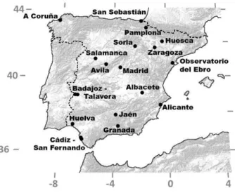
Meanwhile the digitalized time-series become available and, in order to initiate a methodological exploration, we have here selected two eighteen year data subsets of daily maximum temperatures for seventeen meteorological Spanish stations (Fig. 1). The first one covers the period 1904-1921 and the second one 1990-2007, both have missing values but that is a pre-condition which must be included in any exploration of historical data. The empirical distribution

Fig. 1. Distribution of the selected meteorological stations within Spain.

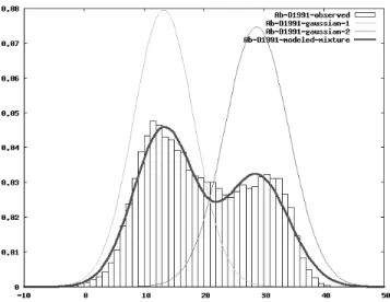
functions (EDF) for many stations are clearly multimodal (Fig. 2). Also, nearly all stations show important changes in the shape of the distribution when compared to the two periods of time. As a first approximation to the study of the complex physical processes which may be responsible for such complex structures and changes, we have simplified the problem, by considering that the EDFs could be explained by the mixing of two normal distributions. The resulting parameters of these distributions, for each station and epoch, have been the inputs for the rest of the present analysis.

III. PROCESSINGMETHODOLOGY

A. Dissection of Mixtures of Probability Distributions

As seen in Section-II (Fig. 2), the empirical distribution functions (EDF) of Tmax data for many stations exhibits

a strong multimodal character. This behavior suggests that the underlying distribution is actually the mixture of several individual distributions.

Letf (x, P) be a probability density function for a random variable _{x, which depends on a set of parameters P. The} mixture f can be expressed as a convex combination of M

Fig. 2. Empirical Distribution Functions (EDF) of Tmax values for the Ab-1991D station (located in Albacete, Fig. 1). Note the strong bimodal character of the EDF.

individual distributionsfi(x, Pi): f (x, P) = M −1 X i=1 [αifi(x, Pi)] + 1 − M −1 X i=1 αi ! fM(x, PM) (1) where P = M [ i=1

Pi andαi ∈ [0, 1], i = 1, 2, . . . , M are the

mixing coefficients satisfying PM

i=1αi = 1. In a simple

model in which the individual DFs are normal distributions withPi = {µi, σi}, fi(x, µi, σi) = 1 (√2π)σi e−12(x−µiσi ) 2 (2) where µi and σi and the respective means and standard

deviations of the constituting distributions. In an attempt at understanding the nature of the Tmax EDFs, a model given

by Eqs. 1-2 with M = 2 was fitted to the data coming from each meteorological station using the Levenberg-Marquardt algorithm [2].

B. Clustering

Hierarchical clustering is a well known family of methods for unsupervised classification [3]. It was used for exploring the structure of the data resulting from the dissection of the EDFs into their Gaussian components, as determined by their means, standards deviations and mixing proportion. Ward’s classical method [4], [3] was used with Euclidean distance. Other clustering techniques were applied as well, but their results were consistent with those obtained with Ward’s method and are not shown.

C. Dimensionality reduction via nonlinear transformations and visualization

One of the steps in the construction of a virtual reality (VR) space for data representation is the transformation of the original set of objects under study O, often defining a heterogeneous high dimensional space, into another space of small dimension ˆO, (typically {2, 3}) with an intuitive metric (e.g. Euclidean). The operation usually involves a non-linear transformation (_{ϕ : O → ˆO); implying some information} loss. There are basically three kinds of spaces sought [5]: i)

spaces preserving the structure of the objects as determined by the original set of attributes or other property, ii) spaces preserving the distribution of an existing class or partition defined over the set of objects and iii) hybrid spaces.

In this study, unsupervised spaces are constructed because data structure is one of the most important elements to con-sider when the location and adjacency relationships between the objects in the new space should give an indication of the

similarity relationships[3], [6] between the objects, as given by the set of original attributes [7]. ϕ can be constructed to maximize some metric/non-metric structure preservation criteria as in multidimensional scaling [8], [6], or to minimize some error measure of information loss [9]. If δij is a

dissimilarity measure between any two objects i, j ∈ O , and ζ_ˆiˆj is another dissimilarity measure defined on objects ˆi, ˆj ∈ ˆO (ˆi = ϕ(i), ˆj = ϕ(j), a frequently used error measure associated to the mapping ϕ is:

Se= 1 P i<jδij P i<j(δij− ζˆiˆj)2 δij (3) When seeking simultaneously for a reduced set of features and a suitable space for visualization, a target 3-D space is the natural choice. In generalϕ is a nonlinear function and in order to compare results from transformations obtained with different algorithms, a canonical representation is preferred. It can be obtained by performing a principal component transformation P after ϕ, so that the overall transformation is given by the composition

ˆ

ϕ = (ϕ ◦ P) (4)

refered to as the canonical mapping.

1) Classical Optimization: The Fletcher-Reeves method is a well known technique used in deterministic optimization [2]. It assumes that the function f is roughly approximated as a quadratic form in the neighborhood of aN dimensional point P. f (~x) ≈ c − ~b · ~x + 12~x · A · ~x, where c ≡ f(P),

b ≡ −∇f|P and[A]ij ≡ ∂

2

f ∂xi∂xj|P

The matrix A whose components are the second partial derivatives of the function is called the Hessian matrix of the function at P. Starting with an arbitrary initial vector~g0

and letting ~h0= ~g0, the conjugate gradient method constructs

two sequences of vectors from the recurrence ~gi+1 = ~gi−

λiA· ~hi, ~hi+1 = ~gi+1− γiA· ~hi, where i = 0, 1, 2, . . .

The vectors satisfy the orthogonality and conjugacy con-ditions~gi· ~gj= 0, ~hi· A · ~hj = 0, ~gi· ~hj= 0, j < i

andλi,γi are given byλi=~_h~g_i·A·~i·~gj_hi, γi=~gi+1_~gi·~_·~g_gi+1_i .

It can be proven [2] that if ~hi is the direction from point

Pi to the minimum of f located at Pi+1, then ~gi+1 =

−∇f(Pi+1), therefore, not requiring the Hessian matrix.

2) Genetic Programming: Genetic programming (GP) techniques aim at evolving computer programs. They are an extension of the Genetic Algorithm introduced in [10] and further elaborated in [11], [12] and [13]. The algorithm starts with a set of randomly created computer programs. This initial population goes through a domain-independent

breeding process over a series of generations. Programs representing functions are of particular interest and can be modeled as y = F (x1, · · · , xn), where (x1, · · · , xn) is

the set of independent or predictor variables, and y the dependent or predicted variable. The function F is built by assembling functional subtrees using a set of predefined primitive functions (the Function Set). In general the model describing the program is given by y = F (~x), where y ∈ and~x ∈ n_.

3) Genetic Programming with Vector Functions: Most implementations of genetic programming for modeling fall within this paradigm but for problems like the ones addressed in this paper vector functions are required. A GP based approach for finding vector functions was presented in [14]. In these cases the model associated to the evolved programs is ~y = F (~x), which allows for the simultaneous estimation of several dependent variables ~y from a set of indepen-dent variables ~x. These are not multi-objective problems, but problems where the fitness function depends on vector variables. The mapping between vectors of two spaces of different dimension (n and m) is one of that kind. In this case a transformation like ψ : n _→ m _{mapping vectors}

~x ∈ n _{to vectors ~y ∈} m _{would allow a reformulation of}

Eq. 3 as: Se= 1 P i<jδij P i<j(δij− d(ψ(~xi), ψ(~xj))2 δij , (5)

In problems of this type, the evolution process works with populations of forests such that the evaluation of the fitness function depends on the set of trees within a forest [14]. Any classical GP can be extended for working with vector functions. In this paper, the vectorial GP with both supervised and unsupervised learning capabilities from [14] was used. This development extends the ECJ System (Evolutionary Computation in Java) [15] and also the Gene Expression Programming technique (GEP) [16], [17].

Two different uses were made of vector-GP: i) Unsuper-vised for obtaining the structure preserving mappings from Eq. 3 (reformulated as Eq. 5) and ii) supervised for producing an explicit approximation of the implicit mapping solution obtained with the Fletcher-Reeves classical optimization method (Section. III-C.1).

IV. EXPERIMENTALSETTINGS

The genetic programming experiments with the ECJ-GEP system for the solution of Eq. 5 (unsupervised problem), were performed using population sizes of {500, 1000} indi-viduals and the number of generations in {50000, 100000}. For each parameter set, 100 random initial population tri-als were made for a total of 400 runs. The remaining algorithm parameters were fixed at the following suggested values [17]: genes/chromosome = 5, gene headsize = 5, elitism = 3 individuals, constants = allowed (in [−1, 1]), probabilities: inversion = 0.1, mutation = 0.044, istranspo-sition = 0.1, ristransposition-prob = 0.1, onepointrecomb-prob = 0.3, twopointrecomb-prob = 0.3, generecomb-prob

=0.1, genetransposition-prob = 0.1, rnc-mutation= 0.01, dc-mutation-prob =0.044, dc-inversion= 0.1, dc-istransposition = 0.1. In particular, the Function Set was very simple, com-posed only of some arithmetic functions complemented by the power and log (base 10) functions: {+, −, ∗, /, ∧, log}.

As a complementary experiment, vector-GP was used to approximate the solution of Eq. 4 (for a 3D space) obtained with the Fletcher-Reeves algorithm (a supervised regression problem, as the target vector elements are given). The population sizes were {100, 300, 500}, the number of generations{10000, 30000, 50000} and the function set was {+, −, ∗, ∧} (simpler). The remaining parameters were the same as those for the unsupervised vector-GP experiment, for a total of900 runs.

The error measure was the mean squared error given by M SE = 1 n n X i=1 (~yi− ψ(~xi))2 (6)

where ~yi is the 3D space vector obtained with the

Fletcher-Reeves algorithm,ψ(~xi) is the one obtained with vector-GP

for the i-th original vector ~xi and n is the total number of

vectors (one/EDF).

V. MAINRESULTS

A. EDF dissection

The model given by Eq. 1 with M = 2 was fitted to the EDFs of the 34 stations (17 for the period 1904-1921 and 17 for 1990-2007) and the parameters of the constituent theoretical distributions with the corresponding mixing rate are shown in Table. I. The first 17 rows (first half of the table) corresponds to 1904-1921, the second half to 1990-2007. Station codes as recognized by AEMET (the Spanish meteorological agency). Codes ending with ’D1991’ correspond to series digitalized in 1991 [18]. They have been partially incorporated into the AEMET dataset.

The result corresponding to station Ab-D1991 (Fig. 2) is shown in Fig. 3.

B. Clustering

The dendrograms of the cluster analysis (Ward linkage, Euclidean distance) of the five variables in Table. I for the two blocks of data are presented in Fig. 4. They have been cut off at a five group level and these classes assigned to the corresponding stations; the geographical distribution is presented in Fig.5.

The general arrangement seems to respond to the influ-ence of Atlantic and Mediterranean waters. The continental climate of Central Spain (class 1-1 in both periods of time) appears grouped with Mediterranean-like conditions (classes 1-). San Sebastian (Ss-D1991), in the humid Northeast, belongs to class 1-3 in the 1904-1921 period; interestingly, a very narrow fringe of Mediterranean vegetation runs along the eastern half of the Bay of Biscay coast. Apparently, the North-Northwest wave regime isolates the waters, which become increasingly warmer along the summer.

Fig. 3. Dissection of the EDF corresponding to station Ab-D1991 according to the gaussian mixture model given by Eq. 1 with M = 2. The solid line is the theoretical mixture model. The constituent gaussian density functions are shown with thin lines. The mixture rate is 0.5625 (see Table. I).

The association of Huelva (Hv-4605), in the Southwest, with Mediterranean-like conditions (class 1-3) in the same 1904-1921 period, it is unclear but, as the station is located some fifteen kilometers from the coast, perhaps it may be easily influenced by the inland Mediterranean conditions. Both stations, however, have become associated with Atlantic conditions (classes 2-1 and 2-2) in 1990-2007.

Cadiz-San Fernando, in the Southwest, appears in 1904-1921 grouped with A Coru˜na, a typical Atlantic station. However, in 1990-2007 they become differentiated even if they still belong to the same ”Atlantic” climatic regime. Apparently, warmer Mediterranean waters, crossing through the Gibraltar Strait, are spreading along the border of the Atlantic coast towards the north [19], modifying the Atlantic climates. Such changes do agree with the observed recent increase in the Western Mediterranean coastal waters tem-perature and the increased temtem-peratures in most of Spanish stations. However, the warming trend is neither uniform nor general, and San Sebastian maximum temperatures have clearly decreased from one period to the other, a pattern also followed by four other stations (Huelva, Jaen, Soria and Huesca): a complex picture which needs further analysis.

Removing the Mixing Rate from the data in Table. I produces important changes in the associations in the South-western stations (Fig. 6). It means that the proportion at which each of the two underlying Gaussian distributions mix is an important factor related to the structural climate change.

C. Dimensionality reduction and unsupervised nonlinear mapping with classical optimization

A dimensionality reduction of the 5-dimensional data matrix of Table. I targeting a 3D space was computed. The transformation sought was the canonical composition of Eq. 4 and it was computed by solving Eq. 3 with the Fletcher-Reeves algorithm followed by a principal components of the resulting 3D matrix. The implicit mapping obtained from the

Station mixingRate mean1 stdv1 mean2 stdv2 Ab-D1991 0.563 12.86 4.82 28.29 5.89 Ac-D1991 0.538 18.03 3.41 27.02 3.32 Av-2444B 0.595 9.17 4.80 23.67 5.80 Ba-D1991 0.367 15.23 3.33 27.93 7.96 Co-D1991 0.226 12.97 1.77 17.72 3.78 Gr-5515A 0.628 14.90 5.00 29.73 4.48 Hc-D1991 0.550 13.20 4.87 27.56 5.33 Hv-4605 0.440 17.81 2.87 27.37 5.03 Ja-D1991 0.676 16.26 5.73 31.70 3.91 Mad-Ret1 0.515 11.57 4.25 26.20 5.95 Obsebre1 0.724 17.67 5.30 28.61 2.54 Pm-9262A 0.177 9.87 2.63 18.19 8.51 Sa-D1991 0.501 11.21 4.42 25.54 6.39 Sf-D1991 0.345 15.82 2.11 23.41 5.21 So-D1991 0.543 9.25 4.74 23.68 5.96 Ss-D1991 0.620 14.17 4.13 21.80 2.88 Zz-9443D 0.496 13.49 4.44 26.73 6.02 Ab-8178D 0.623 15.40 5.65 31.00 4.81 Ac-8025 0.532 19.00 3.43 28.38 3.21 Av-2444 0.661 11.96 5.64 26.65 4.68 Ba-4452 0.430 16.47 3.65 29.68 6.70 Ca-5973 0.255 17.01 1.80 22.88 4.53 Co-1387 0.448 14.38 2.21 20.61 2.91 Gr-5514 0.604 16.35 5.16 31.38 4.83 Hc-9898 0.531 13.05 5.11 27.41 5.88 Hv-4605E 0.283 17.65 2.47 26.36 6.20 Ja-5270B 0.543 14.87 4.43 29.08 5.87 Mad-Ret2 0.505 12.71 4.50 27.42 6.31 Obsebre2 0.704 19.62 5.90 31.23 3.21 Pm-9262 0.241 10.58 3.38 20.25 8.19 Sa-2867 0.564 12.61 4.85 26.95 5.63 So-2030 0.408 9.76 4.30 22.76 7.46 Ss-1024E 0.355 11.30 3.17 19.24 4.13 Zz-9443U 0.541 14.77 4.98 27.87 5.44 TABLE I

EDFDISTRIBUTIONS DISSECTION RESULTS(MEANS,STANDARD DEVIATIONS AND MIXING RATE OF THE THEORETICAL DISTRIBUTIONS

EXTRACTED FROM THE MIXTURE ACCORDING TOEQ. 1). LOCATION CODES: AB: ALBACETE, AC: ALICANTE, AV: AVILA, BA: BADAJOZ, CO:

A CORUNA˜ , GR: GRANADA, HC: HUESCA, HV: HUELVA, JA: JAEN, MAD: MADRID, OBSEBRE: OBSERVATORIO DELEBRO, PM: PAMPLONA,

SA: SALAMANCA, SF: SANFERNANDO, SO: SORIA, SS: SAN SEBASTIAN, ZZ: ZARAGOZA, CA: CADIZ.

solution of Eq. 4 with the Fletcher-Reeves algorithm had a low error value (0.000058), indicating that the new three nonlinear variables retained almost all of the information contained in the five original variables of Table I. Accord-ingly, the 3D representation (impossible to reproduce on hard media) provides a reasonably accurate picture of the structure of the original 5-dimensional data.

A snapshot of the VR space is shown in Fig. 9 (middle). Spheres represent the 1904-1921 stations, whereas the cones represent those from 1990-2007. In this representation two objects (stations) are near if their underlying theoretical Gaussian components have the same properties and if they have been mixed in a similar proportion. In addition, a segment connecting two objects from different time epochs (a sphere and a cone), indicates that they correspond to the same geographical location in Fig. 1, therefore, providing a visual indication of the direction of the time evolution

Fig. 4. Dendrograms for the cluster analysis the EDF dissection data from Table. I using all variables (mean and standard deviations from the dissected distributions and the mixing proportion) Top: 1904-1921 stations. Bottom: 1990-2007 stations.

for each particular location. Wrapper surfaces (in grey) group the 1904-1921 stations (spheres) and the those from 1990-2007 (cones) respectively. Their shift provides a visual representation of the overall spatial and temporal changes in the climate structure experienced in Spain, whereas the individual segments, an indication of the variations at the local scale (the stations’ locations). Clearly, most stations have followed a similar climatic evolution.

A cluster analysis similar to the one performed in the original 5-dimensional space (Ward linkage, Euclidean dis-tance) for each of the two time periods was performed, but this time in the the new nonlinear 3D space gives the dendrograms shown in Fig. 7. The geographical distribution of three classes identified in the dendrograms is shown in Fig. 8. In this case the geographical distributions are simpler and somewhat different from the ones obtained from the clustering of the original five dimensional space, probably a consequence of the space optimization to 3D dimensions. The main difference resides in Central Spain, which in 1904-1921 appears grouped with the cluster branch of Atlantic conditions, whereas in 1990-2007 it is clearly grouped with those having Mediterranean climatic conditions.

Fig. 5. Geographical distribution of classes from the dendrograms of Fig. 4 (black dots indicate the stations of Fig. 1). Class boundaries should be taken only as geographical suggestions. Top: 1904-1921 stations. Bottom: 1990-2007 stations.

D. Dimensionality reduction and unsupervised nonlinear mapping with vector-GP

In order to obtain an explicit representation for Eq. 4 as well as a numeric approximation of the unsupervised, im-plicit canonical mapping obtained with the Fletcher-Reeves algorithm, a solution was computed using the vector-GP approach described in III-C.3. The analytic expressions for the three components of ϕ are given in Eq. 8. Since they represent a solution of Eq. 4, the x, y, z components are ordered in a monotonically decreasing order w.r.t. the vari-ance in the nonlinear 3D space. The best error obtained during the evolutionary experiment was 0.000180 which although larger that the one obtained with the deterministic algorithm, is also very small, indicating a small information loss. The comparison between the 3D spaces obtained with deterministic-implicit mapping and with evolutionary-vector-GP shows non substantial differences (Fig. 9 Middle and Top). Accordingly the explicit solution leads to the same interpretation in terms of the visual representation of the structural time/spatial climate changes at both the regional

Fig. 6. Dendrograms for the cluster analysis of parameters from the EDF dissection for 1904-1921 and 1990-2007 periods, after removal of the Mixing Ratio variable.

and local scale.

ϕx = (((k1∗ µ2+ (log(σ2− k2)/(µ2− µ1))) + log(σ1)) +(k3/(2 ∗ σ1+ µ1+ σ2))) + (k4) ∗ µ2 ϕy = (((k5(log(α)∗k6)+ (k7+ (σ1/(σ1+ µ2)))) + (((k8∗ σ1)(µ2+α))(k9/µ1))) + (k10∗ σ1)/(µ2+ σ1)) +(k11∗ µ1) (7) ϕz = (((log((((k12∗ µ1)/σ1) + (σ1/α))) + (k13∗ σ2)) +(µ2+ (k14− σ1))log(α)) + (k15∗ ((k16/µ1) +σ2))) + k17∗ ((2 ∗ σ1) − (α + µ2))

whereµ1, µ2, σ1andσ2are the mean and standard

devia-tions of the underlying Gaussian distribudevia-tions andα is their mixing rate. There are also several constants:k1= 0.93856,

k2 = 0.92480, k3 = −0.98231, k4 = −0.50368, k5 =

0.02746, k6 = 0.06568, k7 = −0.80294, k8 = 0.08235,

k9 = 0.18920 , k10 = 0.96280, k11 = −0.46218),k12 =

0.28532, k13= 0.40376, k14= −0.12117, k15= −0.83887,

k16= 0.67856, k17= 0.00533.

These equations, although nonlinear, are not excessively complex. The extent to which their algebraic components actually reflect the physics behind the role of the involved variables is an element of great importance. It deserves further investigation.

Fig. 7. Dendrograms for the cluster analysis of the canonical nonlinear transformation of Eq. 4 of the EDF dissection data from Table. I. Top: 1904-1921 stations. Bottom: 1990-2007 stations.

E. Supervised explicit approximation of the implicit unsu-pervised mapping

A complementary experiment was set forth in order to approximate the implicit mapping ϕ produced by theˆ Fletcher-Reeves algorithm used in V-C with a vector-GP explicit mapping (III-C.3). In this supervised problem the resulting nonlinear 3D variables obtained by the Fletcher-Reeves algorithm are learnt with a vector-GP algorithm. The best result has M SE = 0.03536 (Eq. 6 and 3D space of Fig. 9(Bottom)). Note that there is a reasonable good agreement with the target (Fig. 9(Middle)).

ˆ ψx = ((µ2+ k1) ∗ k2)k3+ (σ1k4− (α + k5) − µ1∗ k6) + (k7+ (µ1− σ1) ∗ (α ∗ k8)) + (α − k9) + (µ1+ (k10− α) − k11µ1) ˆ ψy = k12− α ∗ σ2+ (µ1∗ ασ1)k13 + (k(α2∗σ1) 14 − (σ2+ k15)) (8) + (α ∗ k16)σ k17 2 ∗(k18∗σ1)_{+ σ}(k19−k20µ1) 2 ˆ ψz = k21+ (k22+ kα23) + σα (α+1) 1 + k24∗ (σ2∗ σ1+ µ2) + (k24− σ1)

where ψx, ψy, ψz are the approximations ofψ in Eq. 5. The

constants are k1 = 0.80828, k2 = 0.13957, k3 = 1.49598,

k4 = −0.31596, k5 = 0.997555, k6 = 0.99756, k7 =

Fig. 8. Geographical distribution of classes from the dendrograms of Fig. 7 (black dots indicate the stations of Fig. 1). Class boundaries should be taken only as geographical suggestions.

−0.65466, k8 = 0.35535, k9 = 4.32273, k10 = −0.98216, k11 = 0.97894, k12 = 0.74292, k13 = 0.63840, k14 = 0.74757, k15 = −0.77001, k16 = 0.74188, k17= 0.74188, k18 = −0.34977, k19 = 0.99628, k20 = 0.68938. k21 = −0.18373, k22= −0.74782, k23= 0.20437, k24= 0.08398, k24= −0.48972. VI. ACKNOWLEDGEMENTS

The authors thank AEMT (the Spanish Meteorological Agency) and the Ebro Observatory for their help and data.

VII. CONCLUSIONS

Many different processes are intervening in the complex climatic machinery, each one with a different strength, delay. etc. The preliminary results presented here seem to indicate that a combination of statistical procedures with classical optimization and computational intelligence methods like vector genetic programming, provide another perspective to the analysis of daily temperature data. They can be complemented with other procedures like, for example, those presented in [1]. The selection of two data blocks at the

Fig. 9. Canonical 3D spaces obtained by solving Eq. 4 with different algorithms for the original 5D data from Table. I. Stations from the 1904-1921 period are represented with spheres and those from 1990-2007 with vertical cones. The grey wrappers contain the stations from each of the two time periods. The stations belonging to the same geographic location are joined with line segments. Top space: unsupervised vector-GP solution. Middle space: unsupervised solution obtained with the Fletcher-Reeves algorithm. Bottom space: solution obtained by vector-GP supervised by the Fletcher-Reeves’ solution. Note the correspondence between all of the point configurations (distance properties are invariant under coordinate rotations).

beginning and the end of the XX century (of eighteen years each), is a crude, tentative approach, while more compre-hensive and complete datasets of daily temperatures become available. However, the results indicate that there are indeed differences in the climate mechanisms as revealed by the different behavior of the constituent Gaussian distributions of the empirical EDFs. This points towards deeper, more subtle effects than a mere variation in mean temperatures as an indicator of climate change. It is also interesting to note that reasonable accurate visual representation of these complex processes and their changes can be obtained using computational intelligence techniques. They helped in the analysis of spatial and temporal climate changes and suggest possible directions for further investigation.

More elaborated experiments should cover a

continu-ous, sliding time window, which could reveal the possible influence of different physical processes within the data, for instance, the atmospheric circulation system, sea-water temperature variations, anthropic influences, and external forcing. The identification of periods of relatively homoge-neous behavior could be analyzed with local models, looking for possible links with known processes. Further analysis is required in order to more objectively discriminate between anthropic and natural factors in Climatic Change.

The analysis of temperature EDFs based on daily values, their dissection into suitable individual Gaussian components and their investigation with statistical, nonlinear and compu-tational intelligence techniques has a general character and could be applied to other regions.

REFERENCES

[1] J. Vald´es, A. Pou, and R. Orchard, “Characterization of climatic variations in spain at the regional scale: A computational intelligence approach,” in IEEE World Congress on Computational Intelligence

WCCI 2008. 2008 IEEE International Joint Conference on Neural Networks, IEEE. Hong Kong: IEEE, June 1-6 2008.

[2] W. Pres, B. Flannery, S. Teukolsky, and W. Vetterling, Numeric Recipes

in C. Cambridge University Press, 1992.

[3] J. L. Chandon and S. Pinson, Analyse typologique. Th´eorie et

appli-cations. Masson, Paris, 1981.

[4] J. Ward, “Hierarchical grouping to optimize an objective function.” J.

Amm. Stat. Assoc, vol. 58, 1963.

[5] J. Vald´es and A. Barton, “Virtual reality spaces for visual data mining with multiobjective evolutionary optimization: Implicit and explicit function representations mixing unsupervised and supervised properties,” in 2006 IEEE Congress of Evolutionary Computation

(CEC 2006), IEEE. Vancouver, Canada: IEEE, July 16-21 2006. [6] I. Borg and J. Lingoes, Multidimensional similarity structure analysis.

Springer-Verlag, 1987.

[7] J. J. Vald´es, “Virtual reality representation of information systems and decision rules:,” in Lecture Notes in Artificial Intelligence, ser. LNAI, vol. 2639. Springer-Verlag, 2003, pp. 615–618.

[8] J. Kruskal, “Multidimensional scaling by optimizing goodness of fit to a nonmetric hypothesis,” Psichometrika, vol. 29, pp. 1–27, 1964. [9] J. W. Sammon, “A non-linear mapping for data structure analysis,”

IEEE Trans. Computers, vol. C18, pp. 401–408, 1969.

[10] J. Koza, “Hierarchical genetic algorithms operating on populations of computer programs.” in Proceedings of the 11th International Joint

Conference on Artificial Intelligence. San Mateo, CA, 1989. [11] ——, Genetic programming: On the programming of computers by

means of natural selection., MIT Press, 1992.

[12] ——, Genetic programming ii: Automatic discovery of reusable

pro-grams., MIT Press, 1994.

[13] J. Koza, D. Andre, and M. Keane, Genetic programming ii: Automatic

discovery of reusable programs., Morgan Kaufmann, 1999. [14] J. J. Vald´es, R. Orchard, and A. Barton, “Exploring medical data using

visual spaces with genetic programming and implicit functional map-pings,” in Proc. Genetic and Evolutionary Computation Conference

Gecco 2007, 2007.

[15] S. Luke, L. Panait, G. Balan, S. Paus, Z. Skolicki, E. Popovici, J. Harrison, J. Bassett, R. Hubley, , and A. Chircop, ECJ, A

Java-based Evolution Computing Research System, Evolutionary Computation Laboratory, George Mason University., March 2007. [Online]. Available: http://www.cs.gmu.edu/∼eclab/projects/ecj/

[16] C. Ferreira, “Gene expression programming: A new adaptive algorithm for problem solving,” Journal of Complex Systems, vol. 13, 2001. [17] ——, Gene Expression Programming: Mathematical Modeling by an

Artificial Intelligence, Springer Verlag, 2006.

[18] J. J. O˜n_{ate and A. Pou, “Temperature variations in spain since 1901.} a preliminary analysis.” International Journal of Climatology, vol. 16, 1996.

[19] A. L. C. Gonzalez-Pola and M. Vargas-Ya˜n_{ez, “Intense warming and} salinity modification of intermediate water masses in the southeastern corner of the bay of biscay for the period 1992-2003.” J. Geophys.