Non-linear dynamics and contacts of an unbalanced flexible rotor supported on ball bearings
Texte intégral
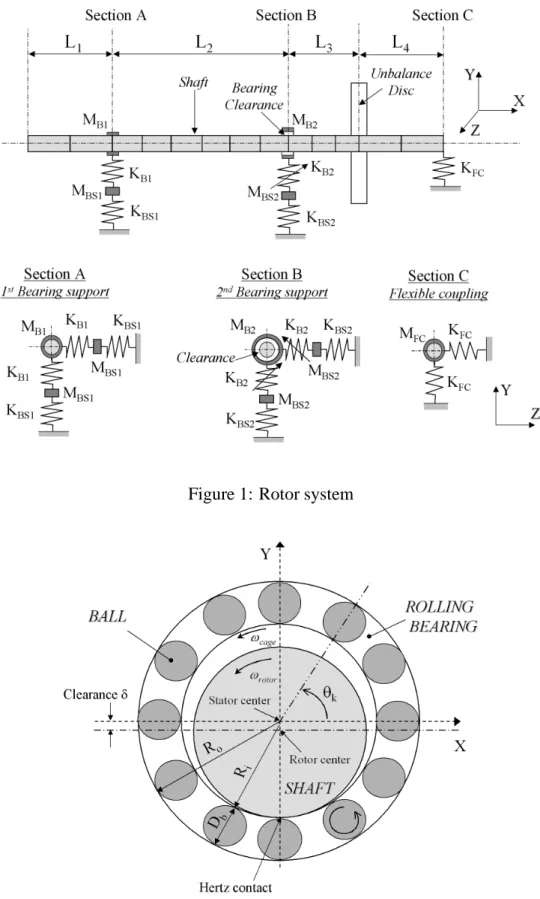
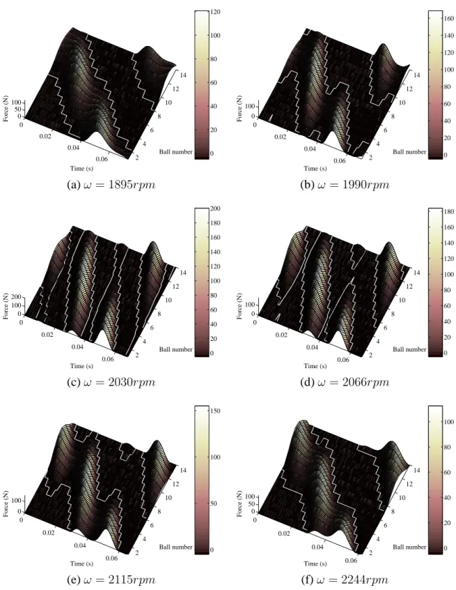
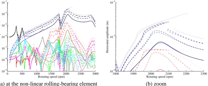
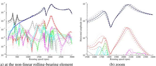
Figure


Documents relatifs
Given the displacement field constructed above for sandwich and laminated beams, a corresponding finite ele- ment is developed in order to analyze the behaviour of lam- inated
In a previous work, the geometric degree of nonconservativity of such systems, defined as the minimal number of kinematic constraints necessary to convert the initial system into
Though numerous studies have dealt with the α− methods, there is still a paucity of publi- cations devoted to the clarification of specific issues in the non-linear regime, such
In addition to the investigation of the influences of the bearing temperature on the dynamics of the flexible rotor at the first critical speeds, a brief investigation into the
So the second part of the paper presents the methodology of the Polynomial Chaos Expansion (PCE) with the Harmonic Balance Method in order to estimate evolu- tions of the n ×
In this paper, sufficient conditions for the robust stabilization of linear and non-linear fractional- order systems with non-linear uncertainty parameters with fractional
In summary, it is fair to say that the factors leading to the right hemispheric specialization for faces in the human adult brain remain largely unclear at present, and cannot be
The real modes CMS procedure, in combination with a shooting/continuation scheme, was used to study the unbalance response and stability of a 24 DOF rotor supported on journal
