Creation of nonlinear density gradients for use in internal wave research

Creation of Nonlinear Density Gradients for Use in Internal Wave Research

By

Victoria Sian Harris

SUBMITTED TO THE DEPARTMENT OF MECHANICAL ENGINEERING IN PARTIAL FULFILLMENT OF THE REQUIREMENTS FOR THE DEGREE OF

BACHELOR OF SCIENCE AT THE

MASSACHUSETTS INSTITUTE OF TECHNOLOGY

JUNE 2007

CVictoria Harris. All rights reserved.

The author hereby grants to MIT permission to reproduce and to distribute publicly paper and electronic copies of this thesis document in whole or in part

in any medium now known or hereafter created.

Signature of Author:

1~

I

JUN 2 1

2007

Lhi

ARIES

Atlantic . Professor of Mechanical Engineering

Thesis Supervisor

N~) _{John H. Lienhard V}

Professor of Mechanical Engineering Chairman, Undergraduate Thesis Committee

-S1CIE

--Creation of Nonlinear Density Gradients for Use in Internal Wave Research

Victoria Sian Harris

Submitted to the Department of Mechanical Engineering

on May 11, 2007 in partial fulfillment of the

requirements for the Degree of Bachelor of Science in

Mechanical Engineering

ABSTRACT

A method was developed to create a nonlinear density gradient in a tank of water. Such gradients are useful for studying internal waves, an ocean phenomenon that plays an important role in climate and ocean circulation.

The method was developed by expanding on the two-tank system currently used to create linear density gradients. A mathematical model of the two-tank system was used and a Matlab script was written to solve the model for the required flow rates in the system given a desired density gradient.

The method was tested by creating three different density gradients: a linear gradient, a hyperbolic gradient, and a two-layer gradient. It was discovered that for a two-layer gradient the flow rates for each layer must be calculated independently of each other, because of problems integrating over a density gradient with a non-continuous slope. It was also discovered that the

system failed at very low flow rates; insufficient mixing in the two-tank system led to gradients weaker than expected. Overall, the measured gradients matched up well with the expected gradients, and it was concluded that the system can successfully produce nonlinear density gradients.

Thesis Supervisor: Thomas Peacock

1.

Introduction

This project's goal is to develop a method of producing a nonlinear density gradient in a tank of salt water, to aid research on internal ocean waves.

The deep ocean does not have uniform density. Instead, it has a smooth density stratification; as you go deeper, the ocean gets denser. When the ocean moves across ridges on the ocean floor, the motion creates waves which propagate up the density stratification. These waves are known as "internal waves."

Until recently, these waves were thought to contribute little to the mixing of the ocean.1 It was thought that the dissipation of energy required to produce the mixing of temperatures in the ocean was associated with turbulence in shallow seas. However, satellite radar altimetry has produced ocean tide maps that tell a different story: the maps imply that while most of the energy is indeed lost in shallow waters, a significant portion is lost over rough topography on the deep ocean floor. It is now thought that these internal waves are more important than wind-generated waves. They play an important role in ocean circulation and climate, and could also hold information about the history of the Earth and the Moon. However, not much is known about the behavior of internal waves.

Internal waves are currently being investigated using tanks in laboratory settings. As of yet, there has not been an easy way to create a nonlinear density gradient to use in these experiments; most have been conducted with a linear gradient, or with linear gradients stacked on top of each other. In this project the two-tank technique used to create a linear density gradient has been expanded using Matlab code and a computer-controlled pump; the result is a method that produces a nonlinear density gradient.

2. Theory

The objective of this project is to produce a nonlinear density gradient in a tank using the two-tank mixing system and computer-controlled pumps. To achieve this, the system must first be modeled using a set of differential equations, following the outline described by D. F. Hill.2 The equations are solved using a Matlab script, which outputs a series of pumping rates. These pumping rates are then sent to the appropriate pump using a LabView program.

Garrett, Chris. "Internal Tides and Ocean Mixing." Science. Vol. 301: 26 September, 2003. Pg 1858.

2 _{Hill, DF. "General Density Gradients in General Domains: The "Two-Tank" Method Revisited." Experiments in}

2.1

The "Two-Tank" Method

Gradient Tank

Salt Tank Mixing Tank

Salt water is pumped Water with gradually into mixing tank increasing density is

pumped into gradient tank Denser layers continually form at bottom of tank, filling tank with water that gets denser as depth increases

Figure 1: The two-tank mixing method

Density gradients for internal wave research are created using the "two-tank" method, as shown in Figure 1. In this method, two tanks are filled with water. One is filled with salt water (the "salt" tank), and one with freshwater (the "mixing" tank), and the two tanks are connected to each other via a pump. A third, empty tank (the "gradient" tank) is connected to the freshwater tank via a second pump. Water from the mixing tank is pumped into the bottom of the empty gradient tank to create a fresh water layer. At the same time, salt water is being pumped from the salt tank to the mixing tank and mixed in with the fresh water in the mixing tank, increasing the overall density of the mixing tank water. Some of this slightly denser water is then pumped into the bottom of the gradient tank, creating a slightly denser layer of water under the freshwater layer already in the gradient tank. This process is continual, with the water in the mixing tank gradually getting denser and adding denser layers to the bottom of the gradient forming in the gradient tank.

This system provides a simple way to create a linear density gradient. If the flow rate from the salt-water tank into the mixing tank is set to exactly half the flow rate from the mixing tank into the gradient tank, the density of the water in the mixing tank with increase linearly in time, which will in turn make a linear density gradient in the gradient tank. If one desires a nonlinear gradient, the two-tank system can still be used, but the system must be described using a system of differential equations and solved numerically, as described in the next section.

Dense (salty) water

Water begins as fresh water, and gets denser as salty

water is mixed in Denser

-0

01

I

Salt Tank Mixing Tank

Flow rate =

Qi

-A___ Flow rate = Q2rr___i

Pump A Pump B Gradient Tank Concentration = C3(z) Volume = V3 Area = A

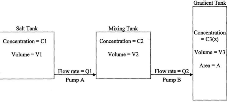
Figure 2: Pumping system block diagram

The pumping system can be modeled by writing equations that relate the various flow rates, salt concentrations, and tank volumes, as shown in Figure 2, to each other. The equations are as follows:

d

d

dt

where the change over time in the amount of salt in the mixing bucket (C2V2) is equal to the amount of salt flowing into the bucket from the saltwater bucket (C1Q1) minus the amount of salt leaving the bucket (C2Q2);

dV2 = Q (t) - Q2 (t) , (2)

dt

where the volume in the mixing bucket changes with the difference between the flow rates of Pump A and Pump B;

A dh = 2 (t) (3)

dt

where A is the cross-sectional area of the gradient tank, h(t) is the height of the water at a given time, and the change in volume of water in the gradient tank is equal to the flow rate into the tank; and

d h(t)

A -

JC

dt ₀

where the change in the amount of salt in the gradient tank is equal to the amount of salt flowing in from the mixing tank.

We assume that Q2(t) is constant and known, that Ci is known, and that the desired gradient C3(z) is known. The initial values of V2 and C2 are also known. The height of the water in the tank can be solved for directly using equation (3):

2.2

Modeling

the Pumping System

Concentration = C1

Volume = Vi

Concentration = C2

h(t) = z = 2 t (5)

A

Equation 5 can be used to convert the density as a function of height, C3(z), into a density function dependent on time. This time-dependent density function describes the density in the mixing tank, C2(t).

Now there are three unknown variables (the volume in the mixing tank V2, the concentration in the mixing tank C2, and the flow rate into the mixing tank Q1), and three equations: (1), (2), and (4). We can use Matlab to solve these equations for our desired variable,

Q1.

2.3 Solving

the

system of equations

The Matlab code used to solve the system of differential equations outlined above can be found with comments in Appendix 1. The script is named "densityD.m." To use the script, the user first sets the level of detail of the gradient (that is, how many individual steps make up the gradient.) Next, the user inputs the desired height of the gradient, and the script breaks this height into a vector with the desired number of steps. The known variables are then set: the constant flow rate from the mixing tank to the gradient tank, Q2, the cross-sectional area of the gradient tank, A, the density of the water in the salt tank, C1, the initial volume in the mixing tank, V2i, and the initial density of the water in the mixing tank, C2i. The desired density gradient, C3(Z), is also set. This vector is interpolated to have the same number of steps as the height vector.

Equation 5 is used to create a time vector with the same number of units as the height vector. The two vectors are equivalent: in one unit of time, a single unit of height will be filled in the tank. This means that the density of the water in the gradient tank as a function of height, C3(z), is equal to the density of the water in the mixing tank as a function of time, C2(t).

Next, equations 1 and 2 are combined to obtain the following equation:

dV

dV

(Q

V

dt C2 -C 1 dt

and that equation is solved for V2 using an ODE solver (and the Matlab function "volume2.m.") From this result, the time derivative of V2 is found. Equation 2 can be then be used to find Q1,

the desired result.

3. Experimental Procedure

3.1

Apparatus

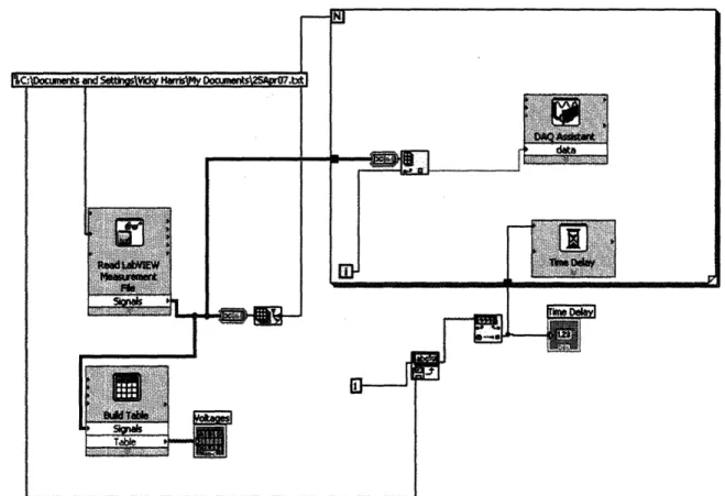
The method for creating a nonlinear density gradient involves a two-tank system with two pumps and a gradient tank. The filling tanks used in this project were square buckets with a maximum capacity of 130 liters. The pumps connecting the salt tank to the mixing tank and the mixing tank to the gradient tank were peristaltic pumps each consisting of a Masterflex 77420-00 Pump Drive with a 77600-62 High Performance Pump Head. The pump that needed a time-varying flow rate was controlled using a LabView VI. The block diagram for the VI, named "PumpControl.vi," is shown in Figure 3:

Figure 3: Block diagram of LabView VI for sending voltage signals to peristaltic pump

The VI reads a file containing the length of the time step and a series of voltages. It strips off the information about the time step and uses the value of the time step to time a "for" loop. The series of voltages is fed, one voltage value at a time via the "for" loop, to an NI-DAQ device that then sends the correct voltage to the peristaltic pump.

The pumps were connected to the buckets via lengths of polyurethane tubing with an inner diameter of 5/8 inches. The gradient tank itself was a rectangular tank measuring 1.3 meters by 0.2 meters, with a height of 0.66 meters.

To measure the density gradient inside the tank, a conductivity and temperature probe was used: a Precision Measurement Engineering Model 125 Microscale Conductivity and Temperature Instrument. The probe was lowered into the tank using a traverse setup that comprised of a Parker ER Series Rodless Actuator and Lin Engineering Step Motor, controlled

by the computer via a Parker E Series E-AC Drive.

Calibration of the probe involved measuring the temperature and density of a series of water samples. The measurements were taken using an Anton Paar 38 Density Meter and an Omega HH42 digital thermometer. The water samples' temperatures were regulated using a pair NESLAB RTE-140 Refrigerated Bath/Circulators.

3.2

Method

3.2.1 Calibrating the Pumps

The two pumps are switched on and left to run to warm up. After an hour of warming up, the two pumps are calibrated. Pump B is calibrated by programming the pump to deliver a

specific volume, and then measuring that volume. If the delivered volume is significantly different from the requested volume, the pump is recalibrated.

Pump A is connected to the computer and its flow rates are calibrated to corresponding voltages. Using a LabView VI, a voltage is sent to the pump for a specific period of time and the resulting pumped volume is measured. The calibration equation is calculated from this data. The calibration equations used in this project were second degree polynomials, and it was assumed that the flow rate was zero when the voltage was set to zero; this was used as set point. An example of a calibration equation follows:

Voltage = -. 0127Q,2 +1.7191Q, (7)

The calibration equation must be updated before calculating the voltage profile.

3.2.2 Calculating the Voltage Profile

The desired density gradient is created as a Matlab vector and run through the "densityD" script, which solves the system of differential equations relating to the two-tank system and calculates the flow rate from the salt tank to the mixing tank as a function of time. The script then uses the calibration formula from Pump A (such as Equation 7) to calculate a series of voltages to be sent to the pump.

3.2.3 Filling the Tank

Figure 4: Experimental setup (aerial view).

The setup of the filling system is shown in Figure 4. The gradient tank is cleaned and dried. Each bucket of the two-tank system is filled to the appropriate volume using tap water. The salt-water bucket is brought to the correct density by adding salt. The tubing is connected to the appropriate outlets. The pumps are then started, Pump B at a predetermined constant rate and Pump A using a LabView VI that sends the voltages calculated by the Matlab code to the pump. Once the LabView VI has finished running, Pump A shuts off automatically and Pump B is switched off manually.

3.2.4 Measuring the Gradient

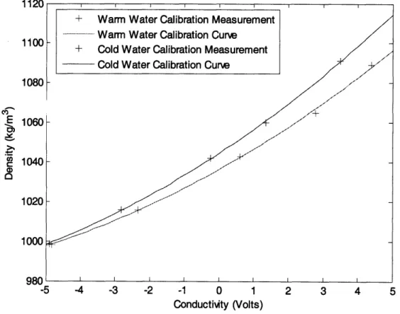
The probe is first calibrated. The calibration is performed using two sets of jars filled with water. The two sets are at temperatures a few degrees above and below room temperature. Each set of jars includes densities ranging from that of fresh water to that of the density in the salt tank. The calibration is performed by measuring the density and temperature of each jar, then using the probe to take each jar's temperature and conductivity. A Matlab script ("profile.m") uses this data to create calibration curves. An example of the calibration curves created is shown in Figure 5:

1120 1 1 1 1

+ Warm Water Calibration Measurement

... W arm W ater Calibration Curve

11000 + Cold Water Calibration Measurement

1080 Cold Water Calibration Curve

1080 -E 1060 '/X E 1040 980 t--_-5 -4 -3 -2 -1 0 1 2 3 4 5 Conductivity (Volts)

Figure 5: Calibration measurements and curves for conductivity/temperature probe.

Following the calibration, the probe is mounted to the traverse above the tank. The probe is lowered to the surface of the water, and then switched on and slowly lowered to the bottom of the tank while data is taken by a LabView VI. The probe is raised to the surface of the water. The probe is then lowered again and a second set of data is taken. The probe is then raised again and switched off. The data is added to the "profile.m" Matlab script, which produces the density gradient of the water in the tank.

4. Results and Discussion

The method described above was tested by attempting to create three different gradients. A linear gradient was attempted, to show that the new method is at least as good as the old method. A hyperbolic gradient was attempted, to investigate the method's ability to generate a nonlinear gradient with continuous slope. Finally, a gradient with two different linear layers was attempted to investigate the method's ability to create a gradient with non-continuous slope.

4.1

Linear Gradient

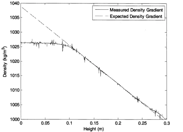
A linear gradient was attempted with the slope of the gradient, dp/dz, equal to 133.33 kg/m4. A flow rate of 1.5 liters per minute into the gradient tank was used as an input variable, and the density of the water in the saltwater tank was adjusted so that the flow rate into the mixing tank remained about constant at about half the flow rate into the gradient tank. This gradient therefore acted as something of a control. The results are shown in Figure 6:

1040 1035 1030 1025 1020 1015 1010 1005 i nnn 0 0.05 0.1 0.15 0.2 0.25 Height (m) 0.3

Figure 6: Expected linear density gradient compared to measured density gradient as a function

of height in the gradient tank.

Figure 6 shows that between the heights of about 0.1 meters and 0.25 meters, the measured gradient matches the predicted gradient very well. A trend line fitted to the data in this range gives the slope of the density gradient to be dp/dz = 134.0 kg/m4, meaning that the error between the slope of the expected gradient and the slope of the measured gradient is 0.5%.

The discrepancy between the two gradients above 0.25 meters can be attributed to the probe used. It is not known why the probe exhibits unusual behavior in this region. It may be because the probe is dry when it first enters the water or has a residue of salt water on it, essentially necessitating a "warm-up" period for the probe. The effect will be seen on subsequent gradient plots. The noise (sharp peaks and valleys) in the experimental result is also due to the probe used, and will also be seen on all the following gradient plots. No method has been developed yet to counteract this noise, but the gradient itself is unaffected.

The bottom 0.1 meters of the experimental gradient show a constant density instead of a linear gradient. This is most likely due to a pump malfunction; Pump A probably became disconnected from the computer and lost the voltage signals, effectively shutting off the pump.

This would cause the density in the mixing tank to stay constant, resulting in constant density instead of a gradient.

4.2 Hyperbolic gradient

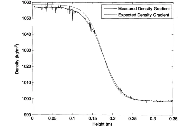
A density gradient with the shape of a hyperbolic tangent was attempted with the following equation for density:

p(z) = -30 tanh(25(z - 0.175)) + 1030

(8)

where z is the depth in the tank in meters and p(z) cubed. The results are shown in Figure 7:

1060 1050 1040 1030 1020 1010 1000 •9Q 0v

is the density at depth z in kilograms per meter

0.05 0.1 0.15 0.2 0.25 0.3

Height (m)

0.35

Figure 7: Comparison

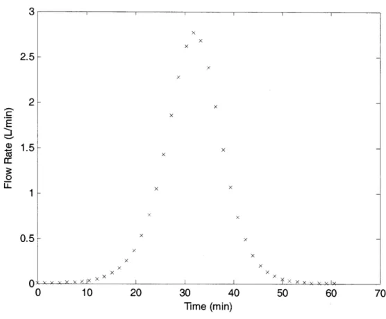
function of height in the tank. of expected hyperbolic density gradient to measured density gradient as a Again, the expected density gradient matches the measured density gradient quite well. The match is especially good in the region from 0.15 meters to 0.35 meters. The linear section between 0.15 meters and 0.2 meters matches well, as does the constant density region from 0.25 meters to 0.35 meters. The curve between 0.2 meters and 0.25 meters is slightly different than expected, but not significantly so. Over the bottom 0.15 meters of the tank, the measured gradient is slightly less dense than expected. This could be due to a variety of factors. As shown in Figure 8, the flow rate into the mixing tank during the last 0.1 meters (approximately the last fifteen minutes of filling) was quite low:

2.5 2 E S1.5 rr 0 1 0.5 (V 0 10 20 30 40 50 60 70 Time (min)

Figure 8: Flow rate into the mixing tank as a function of time for generating the hyperbolic

density gradient.

Because the amount of high density water flowing into the mixing bucket was so low, the mixing pump may not have been strong enough to ensure a uniform density in the mixing bucket. Thus, the water actually being pumped into the gradient tank may not have been as strong as it should have been. The measured density gradient does reach constant density at about the same height as the expected density.

The discrepancy between the gradients may also have been due to one of the pumps varying from its calibration. There were frequent calibration problems with the pumps during early testing. This explanation is unlikely, given that the pumps were given an hour to warm up. Even with the discrepancy in the lower level of the stratification, the measured profile was quite similar to the expected gradient.

4.3 Two-Layer Density Gradient

A two-layer density gradient was attempted. The upper layer of the density gradient was 0.25 meters thick and expected to have a density gradient with dp/dz = 75 kg/m4. The lower layer was 0.1 meters thick and expected to have a density gradient of dp/dz = 500 kg/ m4_{. These}

gradients and the measured gradient are shown in Figure 9:

x x x x x x x x x X -x x x x x / lXX x I Ix x X x X I I I · _

1050 1040 E Y- 1030 u) 1020 1010 4 AlAA 0 0.05 0.1 0.15 0.2 0.25 0.3 0.35 Height (m)

Figure 9: Comparison of the expected linear density gradients to measured linear density gradients as a function of height in the tank.

Figure 9 shows a strong match between the expected upper and lower density gradients and the gradient produced in the tank. In the middle ranges of each density gradient, the matches are strong. The upper gradient has a best-fit slope of dp/dz = 68.8 kg/m4, an error of 8.3%, and

the lower gradient has a best fit slope of dp/dz = 492 kg/ m4, an error of 1.6%. There is a transition phase between the two layers a few centimeters thick; instead of the desired sharp interface the two layers blend together, due to mixing between the layers as they formed. When such a gradient is being used for an internal wave experiment, this transition layer could potentially be siphoned off.

The linear portions of each layer match the expected gradient very well, almost as closely as the match shown in Figure 6, when only one linear density gradient was produced. This is significant because the linear gradient in Section 4.1 was produced by adjusting the density in the saltwater tank so that the flow rate into the mixing tank would be about half that of the flow rate into the gradient tank, mimicking the original two-bucket system. In this case, however, two different gradients were being produced with only one initial density possible in the saltwater tank. The flow rates into the mixing tank were therefore not constant, as shown in Figure 10:

--. - Measured Density Gradient

-- - Expected Lower Density Gradient

5 4 E 3 LL 2 1 n 0 20 40 60 80 100 120 Time (min)

Figure 10: Flow rate into the mixing tank as a function of time for generating the two-layer linear density gradient.

This gradient proved that despite having a rapidly changing flow rate into the mixing tank, it is still possible to produce the same effect as when a constant flow rate is used.

The voltage file used to run the pump and generate the two-layer density gradient was created somewhat differently from previous attempts. The Matlab script does not handle discontinuities in the slope of the density gradient very well. When the desired multi-layer density gradient is inputted all at once, some strange effects are created at the transition points. Figure 11 shows the flow rates outputted by Matlab for the two-layer gradient discussed above, when the two-layer gradient is inputted as one vector:

x x x x x x x xx_xx x IXxxx xX X rr

x x x x x x x x x x x _X x X* ×i X 0 20 40 60 80 100 120 Time (min)

Figure 11: Flow rate into the mixing tank as a function of time for two-layer linear density

gradient (when density gradient is inputted as single vector).

The overall shape of the flow rate in Figure 11 is similar to that of the flow rate in Figure 10 (a low, slowly decreasing flow rate that transitions to a higher, rapidly increasing flow rate), but the transition from one to the other is much messier in Figure 11. There is a transition period of more than six minutes between the two layers. This would have led to an even larger, messier transition layer between the two linear density gradients.

To prevent this problem and produce the cleaner flow rate depicted in Figure 10, the Matlab script was run on each layer separately. The initial conditions were set and the gradient for the upper layer was inputted. The resulting voltages were saved, and then the final conditions from the first layer (specifically, the volume and density in the mixing tank at the end of the creation of the first layer) were inputted as the initial conditions for the second layer. A second series of voltages were generated. The two voltage files were then combined into one, which was used to control the pump.

A difficulty of this method is that if the two layers are of different thicknesses, the Matlab script will produce voltage files with different time steps. This can be resolved by adjusting the 'Refine' value of the ODE solver; the ratios of the Refine values should be as follows:

Thickness of Layer 1 _{'Refine' of Layer 2} Thickness of Layer 2 'Refine' of Layer 1 This gives each layer the same time step.

2.5 2 E u. 0.5 0 ~p#R"~ I

4.4 Problems with Gradients

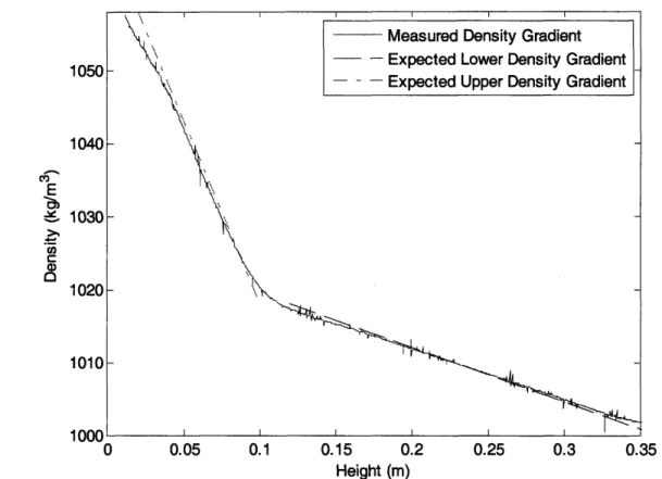
An issue arose when a two-layer stratification was attempted with one very weak layer. In the attempted stratification, the stronger layer had dp/dz = 146.7 kg/m4_{, and the weaker had}

dp/dz = 9.18 kg/m4_{. The very weak layer necessitated a very weak flow rate into the mixing}

tank, even when the flow rate out of the mixing tank was increased. The flow rates are shown in Figure 12: u.o 0.7 0.6 0.5 0.4 0.3 0.2 0.1 n 20 40 60 80 100 Time (min) 120

Figure 12: Flow rate as a function of time for two-layer stratification with one very weak layer.

The weaker layer involves flow rates as low as 0.05 liters per minute. This was too low of a flow rate for the two tank system. The volume pumped was such that the mixing rate in the mixing tank was insufficient, and the water pumped into the gradient tank was at essentially a constant density, as shown in Figure 13:

~n

1016 1014 1012 -- 1010 E 1008 O 1006 1004 1002 • 0nn0 0.05 0.1 0.15 0.2 0.25 0.3 0.35 Height (m)

Figure 13: Comparison of measured density gradient to expected density gradients for a

two-layer density gradient with weak upper two-layer.

The lower layer of the gradient was successful, but the upper layer completely failed. For future gradients, it is important to ensure that the minimum flow rate is high enough (the successful two-layer gradient had a minimum flow rate of 0.125 liters per minute), and that the mixing in the mixing tank is efficient enough.

Other potential problems in the mixing process are easily avoided. After inputting the density gradient into the Matlab code, the outputted flow rate must be checked to be sure that all flow rate values are positive. Similarly, it must be ensured that the volume in the mixing and saltwater tanks will not go too low.

5. Conclusion

The purpose of this project was to develop a method to produce a nonlinear density gradient in a tank of water. The method was created by building on the current two-tank system, using differential equations to describe the flow rates and densities in each part of the system. A Matlab script was written to convert a desired density gradient into a series of flow rates passed to the pumps.

The method was tested by attempting three different gradients - the traditional linear density gradient, a gradient in the shape of a hyperbolic tangent, and a two-layer density gradient. The linear gradient was completely successful. The hyperbolic gradient exhibited small discrepancies from the expected gradient, but overall was successful. The two-layer gradient was very accurate in the linear sections, although the boundary between the two layers was not very sharp. Overall, the method appears successful.

-- Measured Density Gradient _-- - Expected Lower Density Gradient

-- - - Expected Upper Density Gradient

--\

I-l

The method developed in this project could potentially be developed further. The method could be generalized to tanks that do not have a constant cross-sectional area. This could be useful in internal wave research because the topographies used to perturb the density gradient are often quite large; a method that allowed for non-constant cross-sectional area could correct for the effects of that. A more helpful generalization would be adjusting the code to allow for a non-constant flow rate out of the mixing tank. If both pumps had the potential for non-non-constant flow rates, a wider variety of nonlinear gradients could be created, possibly with greater accuracy. The method developed in this project can produce a variety of nonlinear density gradients, and will expand the range of internal wave experiments and allow for a greater understanding of ocean activity.

6. Appendices

6.1

Matlab code

6.1.1 DensityD

%clear all variables before starting clear all

% set the number of levels (both discrete time instants and thus discrete height levels) ns=2000;

% Create a z vector that goes from the top to the base of the tank in ns steps. Coordinate system is set so that z=0 is the top of the tank and depths below the surface are negative z values zbase=-0.3;

dz=zbase/(ns-1);

z = 0:dz:zbase;

% Assign values to the "given" variables global Cl

global Q2

Q2=0.0015/60.0; %Flow rate into the main tank in mA3/s

A = 1.3*0.2; %Area of the tank in mA2

Cl = 1090; %Concentration in the first tank in kg/mA3

V2i = 0.07; % Initial volume in tank 2 in mA3

C2i=1000; % Initial concentration in tank 2 in kg/m^3

ZC3z=input('Enter concentration gradient in main tank'); %asks user for density gradient vector dzi=zbase/(length(C3z)-1); %creates step size based on size of density vector

zi=0:dzi:zbase; %creates depth vector with same number of steps as user-inputted density vector

C3z=interpl(zi,C3z,z); %interpolates user-given density vector into vector that's the same size as the depth and time vectors created at the beginning of the program

% Create a time vector that corresponds to the density profile global C2

global ts

ts=-z*A/Q2; %timing; this makes time steps equivalent to height steps (in one unit of time, one unit of height will be filled)

dt-ts(2)-ts(l); %time interval

C2=C3z; %because time and height steps are equivalent, density in tank 2 changes with time at the same rate that density in tank 3 changes with depth

%Get the time derivative of C2; the first and last values are set equal to those they are adjacent to global C2dot; C2dot = zeros(l,ns); for p=2:l:ns-1 C2dot(p)=(C2(p+1 )-C2(p-1))/2/dt; end C2dot(l)=C2dot(2); C2dot(ns)=C2dot(ns- 1);

%The ODE solver is called; given time range is the time vector, given initial condition is the initial volume in Tank 2.

options = odeset('RelTol', e-4,'AbsTol',le-4, 'Refine',4); %Refine sets the number of divisions in the time vector outputted by the ODE

[T,V2]=ode45(@volume2,[O tmax],V2i,options);

%take the derivative of V2; set initial and final values equal to their adjacent values dT=T(2)-T(1);

V2dot = zeros(1 ,length(V2)); for p=2:1:length(V2)-1 V2dot(p)=(V2(p+l )-V2(p- 1))/2/dT; end V2dot(1)=V2dot(2); V21ength=length(V2); V2dot(V21ength)=V2dot(V21ength-1); %Solve for Q1 Q1 = V2dot+Q2;

%Convert Q1 from cubic meters per second to liters per minute

Q1=Q1 * 1000*60;

figure

plot(T,Q 1 ,'x'); figure

plot(z,C3z);

%Use calibration equation determined from pump to convert flow rate to voltage

%Sub in the voltage calibration equation you find for yourself; the below equation is only an example

voltage=zeros(V21ength, 1); voltage=-.06*Q1.^2+1.7169*Q1; voltage=voltage';

%save a vector whose first value is the time interval and whose remaining values are the voltage vector, for use in LabView

outputfile(1)=dT;

for i=2:length(outputfile) outputfile(i)= voltage(i-1); end;

6.1.2 volume2

%The ODE function is declared function dy = volume2(t,y)

%The global variables are declared global Cl

global C2 global C2dot global Q2 global ts

%The function is initialized dy=zeros(1,1);

%The differential equation: