Supplement of The Cryosphere, 14, 2005–2027, 2020 https://doi.org/10.5194/tc-14-2005-2020-supplement © Author(s) 2020. This work is distributed under the Creative Commons Attribution 4.0 License.
Supplement of
Glacier runoff variations since 1955 in the Maipo River basin, in the
semiarid Andes of central Chile
Álvaro Ayala et al.
Correspondence to:Álvaro Ayala (alvaro.ayala@ceaza.cl)
2
Section S1: Geodetic mass balances
This section presents a summary of the methods included in the study by Farías-Barahona et al. (2020):
Farías-Barahona, D., Ayala, Á., Bravo, C., Vivero, S., Seehaus, T., Vijay, S., Schaefer, M., Buglio, F., Casassa, G. and Braun, 20
M. H.: 60 years of glacier elevation and mass changes in the Maipo River Basin, central Andes of Chile, Remote Sens., In review, 2020.
Derivation of the 1955 DEM
A Digital Elevation Model (DEM) of the Chilean Central Andes was derived from a topographic map at a 1:50,000 scale. The map was based upon aerial photographs taken in 1955 (Hycon flights), as part of an agreement between Chile and the Inter-25
American Geodetic Survey of the United States. The cartography was produced by the Chilean Military Geographic Institute (IGM) using analogue photogrammetric techniques, which requires an operator that stereoscopically reconstructs the imaging geometry using mechanical or optical devices (Mikhail et al., 2001). The vertical reference used mean sea level corresponding to precise trigonometric levelling with theodolites from tide gauge benchmarks located on the Chilean coast. The maps were georeferenced to the PSAD56 datum, UTM projection zone 19S.
30
The generation of Digital Elevation Models (DEMs) for 1955 consists of the following steps (Farías-Barahona et al., 2019): The 1955 topographic maps containing 50-m contour lines were scanned by the IGM at 1200 DPI.
The scanned maps were georeferenced to a common base using standard Geographic Information System (GIS) procedures. The original PSAD 56 datum was converted to the WGS84 datum.
The 50-m contour lines were digitized. 35
The contour lines were interpolated using the kriging method (e.g. Mölg et al., 2017; Farías-Barahona et al., 2019). A DEM with a final resolution of 30 m was then generated from the contours (Farías-Barahona et al., 2019). Derivation of the 2013 DEM
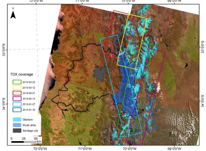
A DEM of the study area for year 2013 was derived from TanDEM-X as follows: A set of TanDEM-X scenes from March 2013 was selected (see Figure S1). 40
The TanDEM-X scenes were processed based on differential SAR interferometry.
The interferograms were filtered and a phase unwrapping procedure was performed using the minimum cost flow algorithm. The data were then converted to differential heights.
3 45
Figure S1. TanDEM-X (TDX) coverage for the Maipo River Basin in 2013. Background image from USGS Landsat 8 satellite data from February 26, 2014.
DEM differencing and uncertainties
The geodetic mass balances for the periods 1955-2000 and 2000-2013 were derived using DEM differencing with the SRTM DEM. This product was obtained by bi-static radar interferometry that were acquired simultaneously in the C-band and X-50
band frequencies between the 11th and 22nd of February 2000 (Farr et al., 2007). This date corresponds to the ablation period in the Southern Hemisphere. Using optical satellite imagery, it was checked that melt-favourable conditions dominated over the Central Andes at the time of the SRTM campaign. The DEMs were co-registered (Nuth and Kääb, 2011) using a mask of stable areas with the Shuttle Radar Topography Mission (SRTM-C) as reference.
The uncertainty in the geodetic mass balances was explicitly quantified based on standard error propagation methods (Braun 55
et al., 2019). Four sources of uncertainty were recognized: i) volume-to-mass conversion, ii) glacier outlines, iii) radar signal penetration of SRTM, and iv) errors in the DEM differencing.
4
Section S2 Additional tables
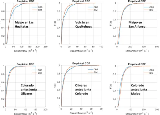
Table S1: Parameters in TOPKAPI-ETH’s sub-surface flux module for the 1955-2016 time period
Parameter
Calibrated value
Units Areas of the Maipo River Basin (*)
Vegetated areas
Non-vegetated areas
Depth 6.5 2.1 °C
Depth (lower layer) 27.6 12.2 m
Vertical hydraulic conductivity at saturation 0.074 0.045 m s-1 Vertical hydraulic conductivity at saturation (lower layer) 0.026 0.056 m s-1 Horizontal hydraulic conductivity at saturation 0.003 0.015 m s-1 Horizontal hydraulic conductivity at saturation (lower layer) 0.438 0.605 m s-1
Water content ratio at saturation 0.65 0.66 -
Water content ratio at saturation (lower layer) 0.66 0.31 -
Residual water content ratio 0.1 0.1 -
Residual water content ratio (lower layer) 0.1 0.1 -
Brooks-Corey exponent for the permeability-saturation curve (horizontal) 3.5 3.5 - Brooks-Corey exponent for the permeability-saturation curve (horizontal)
(lower layer) 3.5 3.5 -
Clapp-Hornberger exponent for the percolation equation (vertical) 13.0 13.0 - Clapp-Hornberger exponent for the percolation equation (vertical) (lower
layer) 13.0 13.0 -
Soil drainage coefficient. Used for upper and lower soil layers 1 1 - Minimum values of soil moisture to have ETA greater zero (ratio
of maximum soil moisture between 0-1) 0.1 0.1 -
Minimum values of soil moisture for ETA to be equal to ETP
(ratio of maximum soil moisture between 0-1) 0.35 0.35 -
(*): The classification was made based on the land use maps developed by the National Forest Corporation (CONAF) 60
5 Table S2: Summary of the performed simulations
Name of simulation Method Domain (*) Period Scenario (**) Comments SIM-1A TOPKAPI-ETH Maipo River Basin 1955-2016 Observed climate
The subperiod 2003-2013 is used for model calibration. The subperiod 1984-2002 is used for model validation. Snow parameters are chosen based on standard values in the literature. Soil parameters are automatically calibrated.
SIM-1B TOPKAPI-ETH Selected glacier x 1955-2000 Observed climate
Parameters SRF and TF are used to fit the geodetic mass balance of each glacier. The rest of the parameters are chosen based on standard values in the literature.
TOPKAPI-ETH Selected glacier x 2000-2016 Observed climate
Parameters SRF and TF are used to fit the geodetic mass balance of each glacier. The rest of the parameters are chosen based on standard values in the literature.
SIM-1C Extrapolation All glaciers
1955-2016
Observed climate
Extrapolation calculated from SIM-1B
SIM-2A TOPKAPI-ETH Maipo River Basin 2000-2099 Synthetic scenario y As in SIM-1A SIM-2B TOPKAPI-ETH Selected glacier x 2000-2099 Synthetic scenario y As in SIM-1B SIM-2C Extrapolation All
glaciers
2000-2099
Synthetic scenario y
Extrapolation calculated from SIM-2B (*): Selected glaciers x go from 1 to 26, (**): Future scenarios y go from 1 to 10.
6
Section S3 Additional model validation
65
We present additional model validation using two datasets: i) six streamflow gauges at intermediate locations of the main catchment, and ii) SWE direct measurements at the Laguna Negra monitoring site of the DGA. The SWE measurements consist of 50 data points measured in the period 1969-2007. While Figure S2 shows the location of the gauges and Laguna Negra in the Maipo River Basin, figures S3 to S7 and Table S3 show results of the validation.
70
While our simulations of SWE at Laguna Negra compare well to the observations (Fig. S6-S7), this is not always the case for the streamflow values. This is partly because there are many water diversions that subtract water from the Maipo River and its tributaries, and some of the available streamflow records at intermediate gauges have not been corrected for these water extractions. However, considering that no specific calibration of the sub-surface parameters for the intermediate river sections was performed, results of the model validation are in general
75
satisfactory at both monthly (Tab. S3 and Fig. S3-S4) and daily (Fig. S5) time scales.
Table S3: Results of the model validation at streamflow gauges at the monthly scale
Gauge Time period Average streamflow (m3 s-1) Nash-Sutcliffe (NS)
Root Mean Square Error (RMSE)
(m3 s-1)
Mean Bias (BIAS)
(%)
Río Maipo en Las Hualtatas 1979-2013 32.3 0.63 15.6 –11.2 Río Volcán en Queltehues 1955-2015 8.1 0.61 6.1 –22.0
Río Maipo en San Alfonso
1955-2015
73.0 0.60 35.8 –12.2
Río Colorado antes junta río Olivares (*)
1978-2016
11.3 0.49 9.9 –23.9
Río Olivares antes junta río Colorado (*)
1978-2016
6.0 0.26 7.0 –4.8
Río Colorado antes junta río Maipo (*)
1955-2015
30.3 0.26 17.4 +19.6
7
Figure S2: Location of intermediate streamflow gauges and the Laguna Negra snow monitoring site. Note that
80
8
Figure S3: Validation of model results at six intermediate streamflow gauges. Monthly time series.
Maipo en Las Hualtatas
Volcán en Queltehues
Maipo en San Alfonso
Colorado antes junta Olivares
Olivares antes junta Colorado
9
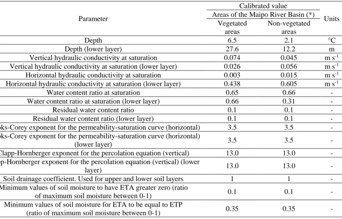
Figure S4: Validation of model results at six intermediate streamflow gauges. Flow-duration curves of monthly
85
time series.
Figure S5: Validation of model results at six intermediate streamflow gauges. Flow-duration curves of daily time series. Maipo en Las Hualtatas Volcán en Queltehues Maipo en San Alfonso Colorado antes junta Olivares Olivares antes junta Colorado Colorado antes junta Maipo Maipo en Las Hualtatas Volcán en Queltehues Maipo en San Alfonso Colorado antes junta Olivares Olivares antes junta Colorado Colorado antes junta Maipo
10 90
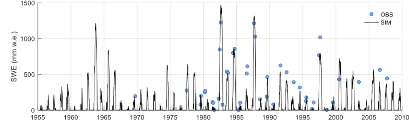
Figure S6: Validation of model results using SWE manual measurements at Laguna Negra (33.67°S, 70.11°W). The SWE measurements consist of 50 data points measured in the period 1969-2007. Daily time series of
simulated values against observations.
Figure S7: Validation of model results using SWE manual measurements at Laguna Negra (33.67°S, 70.11°W).
95
The SWE measurements consist of 50 data points measured in the period 1969-2007. Scatter plot of observations and simulated values at the time of the measurements.
11 References
100
Braun, M. H., Malz, P., Sommer, C., Farías-Barahona, D., Sauter, T., Casassa, G., Soruco, A., Skvarca, P. and Seehaus, T. C.: Constraining glacier elevation and mass changes in South America, Nat. Clim. Chang., 9(2), 130–136, doi:10.1038/s41558-018-0375-7, 2019.
Farías-Barahona, D., Vivero, S., Casassa, G., Schaefer, M., Burger, F., Seehaus, T., Iribarren-Anacona, P., Escobar, F. and Braun, M. H.: Geodetic mass balances and area changes of Echaurren Norte Glacier (Central Andes, Chile) between 1955 and 105
2015, Remote Sens., 11(3), 260, doi:10.3390/rs11030260, 2019.
Farías-Barahona, D., Ayala, Á., Bravo, C., Vivero, S., Seehaus, T., Vijay, S., Schaefer, M., Buglio, F., Casassa, G. and Braun, M. H.: 60 years of glacier elevation and mass changes in the Maipo River Basin, central Andes of Chile, Remote Sens., In review, 2020.
Farr, T., Rosen, P., Caro, E., Crippen, R., Duren, R., Hensley, S., Kobrick, M., Paller, M., Rodriguez, E., Roth, L., Seal, D., 110
Shaffer, S., Shimada, J., Umland, J., Werner, M., Oskin, M., Burbank, D. and Alsdorf, D.: The shuttle radar topography mission, Rev. Geophys., 45(2005), 1–33, doi:10.1029/2005RG000183.1.INTRODUCTION, 2007.
Mikhail, E. M., J.S., B. and McGlone, J. C.: Introduction to modern photogrammetry, John Wiley and Sons Inc., New York., 2001.
Mölg, N., Ceballos, J. L., Huggel, C., Micheletti, N., Rabatel, A. and Zemp, M.: Ten years of monthly mass balance of 115
conejeras glacier, Colombia, and their evaluation using different interpolation methods, Geogr. Ann. Ser. A Phys. Geogr., 99(2), 155–176, doi:10.1080/04353676.2017.1297678, 2017.
Nuth, C. and Kääb: Co-registration and bias corrections of satellite elevation data sets for quantifying glacier thickness change, Cryosph., 5(1), 271–290, doi:10.5194/tc-5-271-2011, 2011.