HAL Id: hal-01418875
https://hal.archives-ouvertes.fr/hal-01418875
Submitted on 17 Dec 2016HAL is a multi-disciplinary open access archive for the deposit and dissemination of sci-entific research documents, whether they are pub-lished or not. The documents may come from teaching and research institutions in France or
L’archive ouverte pluridisciplinaire HAL, est destinée au dépôt et à la diffusion de documents scientifiques de niveau recherche, publiés ou non, émanant des établissements d’enseignement et de recherche français ou étrangers, des laboratoires
Automata-based Verification of Programs with Tree
Updates
Peter Habermehl, Radu Iosif, Tomas Vojnar
To cite this version:
Peter Habermehl, Radu Iosif, Tomas Vojnar. Automata-based Verification of Programs with Tree Updates. Acta Informatica, Springer Verlag, 2010. �hal-01418875�
Noname manuscript No. (will be inserted by the editor)
Peter Habermehl · Radu Iosif · Tom´aˇs Vojnar
Automata-based Verification of Programs
with Tree Updates
the date of receipt and acceptance should be inserted later
Abstract This paper describes a verification framework for Hoare-style pre- and post-conditions of programs manipulating balanced tree-like data structures. Since the considered verification problem is undecidable, we appeal to the standard semi-algorithmic approach in which the user has to provide loop invariants, which are then automatically checked, together with the program pre- and post-conditions. We specify sets of program states, representing tree-like memory configurations, using Tree Automata with Size Constraints (TASC). The main advantage of this new class of tree automata is that they recognise tree languages based on arith-metic reasoning about the lengths (depths) of various (possibly all) paths in trees, like, e.g., in AVL trees or red-black trees. TASCs are closed under union, intersec-tion, and complement, and their emptiness problem is decidable. Thus we obtain a class of automata which are an interesting theoretical contribution by itself. Fur-ther, we show that, under few restrictions, one can automatically compute the ef-fect of tree-updating program statements on the set of configurations represented by a TASC, which makes TASC a practical verification tool. We tried out our ap-proach on the insertion procedure for red-black trees, for which we verified that the output on an arbitrary balanced red-black tree is also a balanced red-black tree.
A short version of this paper appeared in the Proceedings of TACAS 2006. The work was sup-ported by the French Ministry of Research (RNTL project AVERILES), the Czech Science Foundation within the project 102/07/0322, the Czech-French Barrande project MEB 020840, and the Czech Ministry of Education by the project MSM 0021630528.
P. Habermehl
LIAFA, Universit´e Paris Diderot—Paris 7/CNRS, Case 7014, F-75205 Paris 13, France, E-mail: [email protected]
R. Iosif
VERIMAG, Universit´e Joseph Fourier/CNRS/INPG, 2 av. de Vignate, F-38610 Gi`eres, France, E-mail: [email protected]
T. Vojnar
FIT, Brno University of Technology, Boˇzetˇechova 2, CZ-61266, Brno, Czech Republic, E-mail: [email protected]
1 Introduction
Verification of programs using dynamic memory primitives, such as allocation, deallocation, and pointer manipulations, is crucial for a feasible method of soft-ware verification. In this paper, we address the problem of proving correctness of programs that manipulate balanced tree-like data structures. Such structures are very often applied to implement in an efficient way lookup tables, associa-tive arrays, sets, or similar higher-level structures, especially when they are used in critical applications like real-time systems, kernels of operating systems, etc. Therefore, a number of such search tree structures like the AVL trees, red-black trees, splay trees, and so on [11] have been introduced.
Tree automata [9] are a powerful formalism for specifying and reasoning about infinite sets of trees. However, there are two major obstacles against the broad use of tree automata in program verification:
– Imperative programs perform destructive updates of selector fields, changing a tree-shaped data structure by temporarily introducing sharing of branches and/or loops. For instance, this is the case of tree rotations [23] which are implemented as a finite sequence of selector updates introducing a loop in the tree in order to re-establish the tree-like shape later on.
– Tree automata represent regular sets of trees, which is not sufficient when one needs to reason in terms of balanced trees as in the case of AVL and red-black tree algorithms.
In order to overcome the first problem, we observe that most algorithms work-ing on balanced trees [11] use tree rotations and addition/removal of leaf nodes to/from a tree as the only operations that change the structure of the input tree. In our framework, we consider these updates as single (atomic) steps in the program. The correctness of their implementation, using lower-level pointer operations, can, however, be checked separately in a different formalism such as, for example, 3-valued predicate logic with transitive closure [24], or tree automata extended with additional “routing” expressions on the tree backbone as in [17] or in [5], where the so-called abstract regular tree model checking is used.
The second inconvenience is solved in the present paper by introducing a novel class of tree automata, called Tree Automata with Size Constraints (TASC). TASC are tree automata whose actions are triggered by arithmetic constraints involving the sizes of the subtrees at the current node. The size of a tree is a numerical func-tion defined inductively on the tree structure such as, for instance, the height, the maximum number of black nodes on all paths, etc. The main advantage of using TASC in program verification is that they recognise non-regular sets of tree lan-guages, such as the AVL trees, the red-black trees, and, in general, sets of trees involving arithmetic reasoning about the lengths (depths) of various (possibly all) paths in the trees. We show that the class of TASC is closed under the operations of union, intersection, and complement. Also, the emptiness problem is decidable. We thus obtain a class of automata which are a significant theoretical contribution by itself. Moreover, the semantics of the programs performing tree updates (node recolouring, rotations, leaf nodes appending/removal) can be effectively repre-sented as changes on the structure of the automata.
In our verification approach based on TASC, the user has to provide the pre-condition and postpre-condition of the (sequential) imperative program being verified
as well as loop invariants for all loops present in the program. The verification problem then consists in checking validity of Hoare triples of the form {P}C{Q}, where P and Q are TASC-encoded sets of configurations corresponding to the precondition or postcondition of the program or to some loop invariant, and C is a loop-free fragment of the program to be verified. Next, we reduce this ver-ification problem to the TASC language emptiness problem. Note that while the pre- and postconditions and loop invariants are to be specified by the user, check-ing the validity of the verification conditions is fully automated and exact in our framework.
We tested our approach on an example of the insertion algorithm for the red-black trees, for which we verify that for a balanced red-red-black tree input, the output of the insertion algorithm is also a balanced red-black tree, i.e., the number of black nodes is the same on each path.
Related Work. Sound verification of complex properties of programs handling re-cursive tree-shaped (and other kinds of) data structures—such as verifying that programs implementing advanced search data structures like AVL-trees or red-black trees indeed assure their defining properties, including balancedness—is currently beyond the capabalities of the common program verifiers associated with specification languages like JML [6] or Spec# [3]. These systems can ver-ify in a semi-automatic way (as the user has to provide loop invariants) simpler properties like absence of null-pointer exceptions only. There are approaches, such as [15] or [13], considering verification of even the complex properties of the advanced data structures via testing or model checking, but these approaches are unsound as they work with bounded sets of instances of the data structures only.
Research on possibilities of sound verification of programs that handle com-plex tree-like structures has attracted researchers with various backgrounds, such as static analysis [19,23], proof theory [7], and formal language theory [17,5]. The approach that is the closest to ours is probably the one of PALE (Pointer Asser-tion Logic Engine) [17], which consists in translating the verificaAsser-tion problem into the logic SkS [22] and using tree automata (although the classical ones only) to solve it. Our approach resembles PALE also in that we expect the user to provide the pre-, post-conditions, and the loop invariants, and that we reduce the validity problem for Hoare triples to the language emptiness problem. However, the use of the novel class of tree automata with arithmetic guards allows us to encode quantitative properties such as tree balancing that are not tackled in PALE.
In [23], a specialised framework of quantitative shape analysis based on ab-stract interpretation is introduced in order to verify manipulation of AVL trees. In [2], verification of some properties of inserting into red-black trees (including balancedness) is also reported. The work uses graph rewriting systems for describ-ing the insertion procedure—the model is manually constructed. Then, an overap-proximation using Petri graphs (Petri Nets with additional hypergraph structure) is used for verifying the fact that two red nodes never appear in succession. Further, graph type systems are used to check the balancedness. Not all desirable safety properties are covered this way, and both of the steps require a significant user involvement.
Recently, [16] has proposed an approach for verifying algorithms on balanced trees (and, in particular, on red-black trees) based on decidable theories of term algebras with Presburger arithmetic. These theories allow one to define functions from terms to integers, e.g., the maximal number of black nodes in paths from the root to a leave in a tree. The framework of [16], however, does not allow one to express local updates at an arbitrary control location, which consequently leads to a necessity of using an informal induction when proving program verification conditions. In other recent work [18], a different formal model – in particular, an extension of Separation Logic [?] with user-definable recursive shape predicates – is used to reason about safety of pointer-manipulating programs including inser-tion for red-black trees. This approach also targets the verificainser-tion of Hoare triples in presence of user-specified program invariants. However, checking the verifica-tion condiverifica-tions in this setting is done via sound, but incomplete proof rules, since the decidability status of the underlying logic is unknown.
The definition of TASC is a result of searching for a class of counter tree automata that combines interesting closure properties (union, intersection, com-plementation) with decidability of the emptiness problem. Existing works on ex-tending tree automata with counters (e.g., [12,25]) have mostly concentrated on in-breadth counting of nodes with applications on verifying consistency of XML documents. Our work gives the possibility of in-depth counting in order to express balancing of recursive tree structures. It is worth noticing that similar computation models, such as alternating multi-tape and counter automata, have undecidable emptiness problems in the presence of two or more 1-letter input tapes, or, equiva-lently, non-increasing counters [20]1. However, restricting the number of counters
is problematic for obtaining the closure of automata under intersection. The solu-tion we adopt here is to let the acsolu-tions of the counters depend exclusively on the input tree alphabet, in other words, to encode them directly in the input as size functions. This solution can be seen as a generalisation of the visibly pushdown languages [1] to trees, for singleton stack alphabets. A similar approach has been recently taken in [10], where visibly tree automata with memory (VTAM) have been introduced. VTAM define a subclass of tree automata with one memory [8] enjoying boolean closure properties. Red-black trees and other balanced tree sets can be recognised using this formalism. However, the work in [10] does not di-rectly address the verification of tree-manipulating programs, as it does not give a method to represent the effect of program statements on a set of trees represented as a tree automaton.
Roadmap. In Section 2, we summarise our verification methodology and describe our case study of insertion into red-black trees, which we will use in the paper. In Section 3, we introduce the notion of tree automata with size constraints. Section 4 provides results on determinisation of TASC, discusses their closure properties, and shows that their emptiness is decidable. In Section 5, it is shown how the semantics of tree manipulating programs can be encoded using TASC. Section 6 describes the use of TASC within the chosen case study. Finally, Section 7 contains some concluding remarks, including the future work.
1 This result improves on the early work on alternating multi-tape automata recognising
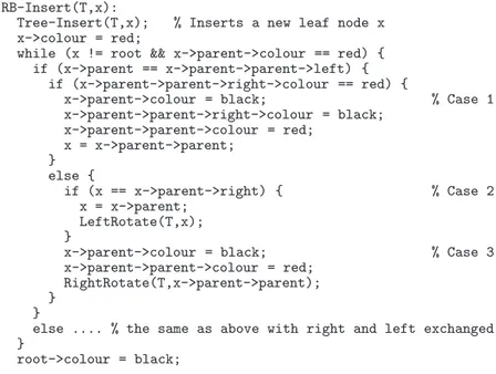
nil nil nil nil nil nil nil nil 8 10 18 15 19 27 5 y x x y ! " # ! " # RightRotate(T,y) LeftRotate(T’,x) (a) (b) T: T’:
Fig. 1 (a) A red-black tree—nodes 10, 15, 19 are red, (b) the left and right tree rotation
2 A TASC-based Verification Methodology and a Running Example
In this section, we introduce our verification methodology for programs using balanced trees. In practice, several data structures based on balanced trees are commonly used, e.g., AVL trees. Here, we will use red-black trees as our running example. Red-black trees are binary search trees whose nodes are coloured by red or black. They are approximately balanced by constraining the way nodes can be coloured. The constraints insure that no maximal path can be more than twice longer than any other path.
More precisely, red-black trees are binary search trees whose nodes contain an element of an ordered data domain, a colour, a left and right pointer, and a pointer to its parent, and that satisfy the following properties:
1. Every node is either red or black. 2. The root is black.
3. Every leaf is black.
4. If a node is red, both its children are black.
5. Each path from the root to a leaf contains the same number of black nodes. An example of a red-black tree is given in Figure 1 (a). The main operations on balanced trees (and hence also red-black trees) are searching, insertion, and deletion. When implementing the last two operations, one has to make sure that the trees remain balanced. This is usually done using tree rotations—cf. Figure 1 (b), which, in the case of red-black trees, can change the number of black nodes on a given path.
Because of the last condition on red-black trees mentioned above (i.e., having the same number of black nodes in each path), it is obvious that the set of red-black trees is not regular, i.e., not recognisable by standard tree automata [9]. Therefore, we have to introduce a tree automata model able to describe sets of (heap) configurations containing balanced trees. This model has to be powerful enough to describe these trees while still having properties allowing for automatic verification (i.e., decidability of inclusion, closure under some operations, etc.).
Here, we define such a class of extended tree automata—namely, tree automata with size constraints (TASC). We suppose the data content of the nodes to be ab-stracted away—we do not verify sortedness. Basic program blocks (i.e., individual program statements or groups of statements that we view as atomic like, e.g., ro-tations) define effective transformations on TASC.
We assume the user to specify the precondition and postcondition of the pro-gram to be verified. Further, we suppose the user to supply an invariant for each loop. The preconditions and postconditions as well as loop invariants are speci-fied by TASC. Then, the verification is performed by automatically checking the validity of each triple {P} C {Q}, where:
– P is the program precondition or a loop invariant, – Q is the program postcondition or a loop invariant, and – C is a loop-free fragment of the code between P and Q.
This is done by computing the image of the precondition after an application of the code of the program block and by checking that the image implies the post-condition. This check is done using language inclusion for TASC.
In Figure 2, we give the pseudo-code of the inserting operation for red-black trees [11]. For this program, we want to show that after an insertion of a node, a red-black tree remains a red-black tree. In our work, we restrict ourselves to calculating the effects of program blocks which preserve the tree structure of the heap. This is not the case in general since pointer operations can temporarily break the tree structure, e.g., in the code for performing a rotation. The operations that we handle are the following:
1. tests on the tree structure (likex->parent == x->parent->parent->left), 2. changing data of a node (as, e.g., recolouring of a nodex->colour = red), 3. left and right rotations (Figure 1 (b)),
4. moving a pointer up or down a tree structure (likex = x->parent->parent), 5. low-level insertion/deletion, i.e., the physical addition/removal of a terminal
node, that is then followed by re-balancing operations. 3 Tree Automata with Size Constraints
In what follows, we work with the set D of all boolean combinations of formulae of the form x −y"c or x"c, for some c ∈ Z and " ∈ {≤,≥}. We introduce equality as x − y = c : x − y ≤ c ∧ x − y ≥ c. Notice that negation can be eliminated from any formula of D since x − y '≤ c ⇐⇒ x − y ≥ c + 1. Also, any constraint of the form x − y ≥ c can be equivalently written as y − x ≤ −c. For a closed formula ϕ, we write |= ϕ to denote that ϕ is valid, i.e., equivalent to true.
A ranked alphabetΣ is a set of symbols together with a function # : Σ → N. For f ∈ Σ, the value #( f ) is said to be the arity of f . Symbols of zero arity are referred to as constants. We denote byΣnthe set of all symbols of arity n fromΣ.
Letλ denote the empty sequence. A tree t over an alphabet Σ is a partial mapping t : N∗→ Σ that satisfies the following conditions:
– dom(t) is a finite prefix-closed subset of N∗, and
– for each p ∈ dom(t), if #(t(p)) = n > 0, then {i | pi ∈ dom(t)} = {1,...,n}. A special case of a ranked alphabet is the binary alphabet in which all symbols have arities either zero or two. Trees over binary alphabets are referred to as binary trees.
A subtree of t starting at a position p ∈ dom(t) is a tree t|pdefined as t|p(q) =
RB-Insert(T,x):
Tree-Insert(T,x); % Inserts a new leaf node x
x->colour = red;
while (x != root && x->parent->colour == red) { if (x->parent == x->parent->parent->left) {
if (x->parent->parent->right->colour == red) {
x->parent->colour = black; % Case 1
x->parent->parent->right->colour = black; x->parent->parent->colour = red; x = x->parent->parent; } else { if (x == x->parent->right) { % Case 2 x = x->parent; LeftRotate(T,x); }
x->parent->colour = black; % Case 3
x->parent->parent->colour = red; RightRotate(T,x->parent->parent); }
}
else .... % the same as above with right and left exchanged }
root->colour = black;
Fig. 2 A procedure for inserting into red-black trees
we define the frontier of P as the set f r(P) = {p ∈ P | ∀i ∈ N pi '∈ P} i.e., the set of tree positions from P whose direct successors are not in P any longer. For a tree t, we use f r(t) as a shortcut for f r(dom(t)). If t is a tree andp = .p1, . . .,pn/
is a sequence of positions pi∈ dom(t), we denote by t •p.t1, . . . ,tn/ the result of
replacing each subtree t|piby tifor all 1 ≤ i ≤ n. We denote by T(Σ) the set of all
trees over the alphabetΣ.
Intuitivelly, a tree mapping is a generalisation of a homomorphism that maps each position from the domain of the source tree into a subtree of the destination tree:
Definition 1 Given two trees t : N∗→ Σ and t0: N∗→ Σ0, a function h : dom(t) →
dom(t0) is said to be a tree mapping between t and t0if the following holds:
– h(λ) = λ, and
– for any p ∈ dom(t), if #(t(p)) = n > 0, then there exists a prefix-closed set Q ⊆ N∗such that pQ ⊆ dom(t0) and h(pi) ∈ f r(pQ) for all 1 ≤ i ≤ n.
A size function (or measure) associates to every tree t ∈ T(Σ) an integer |t| ∈ Z. Size functions are defined inductively on the structure of the tree. For each f ∈ Σ, if #( f ) = 0, then | f | is a constant cf, otherwise, for #( f ) = n, we have:
| f (t1, . . . ,tn)| = b1|t1| + c1if |= δ1(|t1|,...,|tn|) . . . bn|tn| + cnif |= δn(|t1|,...,|tn|)
where b1, . . . ,bn∈ {0,1}, c1, . . . ,cn∈ Z, and δ1, . . . ,δn∈ D, all depending on f .
In order to have a consistent definition, it is required thatδ1, . . . ,δndefine a
parti-tion of Nn, i.e., |= ∀x
δj(x1, . . . ,xn)).2A sized alphabet (Σ,|.|) is a ranked alphabet with an associated
size function.
Example. The height of a binary tree is an example of a tree measure, defined as |c| = 1, if #(c) = 0, and | f (t1,t2)| = & |t1| + 1 if |t1| ≥ |t2| |t2| + 1 if |t2| < |t1| if #( f ) = 2.
A tree automaton with size constraints (TASC) over a sized alphabet (Σ,|.|) is a 3-tuple A = (Q,∆,F) where Q is a finite set of states, F ⊆ Q is a designated set of final states, and∆ is a set of transition rules of the form f (q1, . . . ,qn)−−−−−−−−−−→ϕ(|1|,...,|n|)
q, where f ∈ Σ, #( f ) = n, and ϕ ∈ D is a formula with n free variables. For con-stant symbols a ∈ Σ, #(a) = 0, the automaton has unconstrained rules of the form a −→ q.
A run of A over a tree t : N∗→ Σ is a mapping π : dom(t) → Q such that, for
each position p ∈ dom(t), where q = π(p), we have:
– if #(t(p)) = n > 0 and qi=π(pi), 1 ≤ i ≤ n, then ∆ has a rule
t(p)(q1, . . . ,qn)−−−−−−−−−−→ q and |= ϕ(|tϕ(|1|,...,|n|) |p1|,...,|t|pn|),
– otherwise, if #(t(p)) = 0, then ∆ has a rule t(p) −→ q.
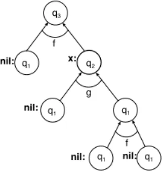
A runπ is said to be accepting if and only if π(λ) ∈ F. As usual, the language of A, denoted as L (A) is the set of all trees over which A has an accepting run. Example. The following TASC recognises the set of all balanced red-black trees. LetΣ = {red,black,null} with #(red) = #(black) = 2 and #(null) = 0. First, we define the size function to be the maximal number of black nodes from the root to a leaf: |null| = 1, |red(t1,t2)| = max(|t1|,|t2|), and |black(t1,t2)| = max(|t1|,|t2|)+1.
The TASC recognising the set of all balanced red-black trees may now be defined as Arb= ({qb,qr},∆ ,{qb}) with the set of transition rules:
∆ = {null −→ qb,black(qb/r,qb/r) |−−−−−−→ q1| = |2| b,red(qb,qb) |−−−−−−→ q1| = |2| r}
By using qx/y within the left-hand side of a transition rule, we mean the set of
rules in which either qxor qytake the place of qx/y. 12
Finally, for binary trees only, we define the notion of balance. For a given binary tree t and a position p ∈ dom(t), we define the balance of t at p as the difference |t|p0| − |t|p1| between the sizes of the left and right subtrees of p.
2 For technical reasons related to the decidability of the emptiness problem for TASC, we do
4 Closure Properties and Decidability of TASC
This section is devoted to the closure of the class of TASC under the operations of union, intersection, and complement. The decidability of the emptiness problem is also proved.
4.1 Determinisation
A TASC is said to be deterministic if, for every input tree, the automaton has at most one run. For every TASC A, we can effectively construct a deterministic TASC Ad such that L (A) = L (Ad). We adapt the classical subset construction
for determinising bottom-up tree automata. We have to take into account the fact that in a deterministic TASC, two rules which have the same left-hand side should not be applicable simultaneously. This problem is solved below by constructing guards of transition rules of the deterministic TASC as conjunctions of the original transition guards, which could otherwise be in a conflict, and their negations in all possible combinations. This way, we ensure that all transitions with the same left-hand side have guards that can never be satisfied simultaneously.
Concretely, let A = (Q,∆,F). We define Ad= (Qd,∆d,Fd) where Qd= P(Q),
Fd= {s ∈ Qd| s ∩ F '= /0}, and f (s1, . . . ,sn)−→ s ∈ ∆ϕ dif and only if:
s ⊆ {q| f (q1, . . . ,qn)−→ q ∈ ∆ ,qψ i∈ si}, and s '= /0
ϕ =%{ψ| f (q1, . . . ,qn)−→ q ∈ ∆ ,qψ i∈ si, q ∈ s} ∧ %
{¬ψ| f (q1, . . . ,qn)−→ q ∈ ∆ ,qψ i∈ si, q '∈ s}
In the case of transition rules involving constant symbols, we have a −→ s ∈ ∆dif
and only if s = {q |a −→ q ∈ ∆ }. The following theorem proves that non-deterministic and deterministic TASC recognise exactly the same languages.
Theorem 1 Adis deterministic and L (Ad) = L (A).
Proof (1) To prove that Adis deterministic, suppose t ∗−−→
Ad
s and t ∗−−→ Ad
s0, for some
t ∈ T(Σ) and two states s,s0∈ Qd. We prove s = s0by induction on the structure
of t. If t = a ∈ Σ0, we have s = s0= {q ∈ Q | a −→
A q} by definition of Ad. Other-wise, let t = f (t1, . . . ,tn) for some f ∈ Σnand t1, . . . ,tn∈ T (Σ), and, by induction
hypothesis, there exist unique states si∈ Qd such that ti−−→∗
Ad
si, 1 ≤ i ≤ n.
Sup-pose that s '= s0, that is, there exists a state q ∈ Q which either belongs to s and
does not belong to s0 or vice-versa. Let us consider the first case, the other one
f (s1, . . .,sn) ϕ 0
−→ s0, and A has a rule f (q1, . . . ,qn)−→ q, for some qψ i∈ si, 1 ≤ i ≤ n,
such thatϕ ⇒ ψ and ϕ0⇒ ¬ψ. But since s and s0are reachable from t in Ad, it
must be the case that |= ϕ(|t1|,...,|tn|) and |= ϕ0(|t1|,...,|tn|), which leads to a
contradiction. Hence s = s0.
(2) “L (Ad) ⊆ L (A)”. We prove inductively that, for all t ∈ T(Σ) and s ∈ Qdsuch
that t ∗−−→
Ad s, for all q ∈ s, we have t ∗−→A q. If t = a ∈ Σ0
, by definition of Ad, we have
s = {q | a −→
A q}. Otherwise, t = f (t1, . . . ,tn) for some f ∈ Σnand t1, . . . ,tn∈ T (Σ), and ti−−→∗
Ad
si, 1 ≤ i ≤ n. By induction hypothesis, for all qi∈ si, we have ti−→∗
A qi. By definition of Ad, there exists a rule r : f (s1, . . . ,sn)−→ s such that, for eachϕ
rule f (q1, . . . ,qn)−→ q with qψ i∈ siand q ∈ s, we have ϕ ⇒ ψ. Moreover, the rule
r is applicable for the subtrees t1, . . . ,tn, i.e., |= ϕ(|t1|,...,|tn|). Hence, each rule
f (q1, . . . ,qn)−→ q is applicable. Therefore, for all q ∈ s, we have t ∗ψ −→
A q. If s ∈ Fd, then, by the definition of Ad, there exists q ∈ s ∩ F. Thus t is accepted by A if it is
accepted by Ad.
“L (Ad) ⊇ L (A)”. We prove inductively that, for all t ∈ T(Σ) and q ∈ Q, if
t ∗−→
A q, then there exists s ∈ Qd such that t ∗−−→Ad s and q ∈ s. If t = a ∈ Σ0
, we have s = {q | a −→ q} and ϕ = 5. Otherwise, t = f (t1, . . . ,tn) for some f ∈ Σn
and t1, . . .,tn∈ T(Σ), and ti−→∗
A qi, for some qi∈ Q, 1 ≤ i ≤ n. By the induction hypothesis, there exist some si∈ Qd such that ti−−→∗
Ad
si and qi∈ si. Also, if t ∗−→
A f (q1, . . . ,qn)−→ψ
A q, then |= ψ(|t1|,...,|tn|). Consider now the set of guards G = {ψ0| ∃q1∈ s1, . . . ,∃qn∈ sn∃q0∈ Q. f (q1, . . . ,qn) ψ
0
−−→
A q0}, and Γψbe the set of all subsets of G that contain ψ. For any set of guards I , we denote byΨI the formula %
ϕ∈Iϕ ∧%ϕ∈G \I¬ϕ. Obviously, ψ =$I∈ΓψΨI. Since |= ψ(|t1|,...,|tn|), there
exists some I ∈ Γψ such that |= ΨI(|t1|,...,|tn|). Now, let s = {q0|∃q1∈ s1, . . . ,
∃qn∈ sn. f (q1, . . . ,qn) ψ 0
−−→
A q0, ψ0∈ I }, and ϕ = ΨI. Notice that q ∈ s. By the definition of Ad, there exists a rule f (s1, . . . ,sn)−→ s in ∆ϕ d, and, moreover, it is
applicable, hence t ∗−−→ Ad
s. By the definition of Ad, if q ∈ F, then s ∈ Fd, hence t is
4.2 Union, Intersection, and Complementation
Let us have two arbitrary TASCs A1= (Q1,∆1,F1) and A2= (Q2,∆2,F2). We can
assume w.l.o.g. that Q1and Q2are disjoint. Let A1∪ A2= (Q1∪ Q2,∆1∪ ∆2,F1∪
F2).
Lemma 1 Given a sized alphabet Σ and two TASCs Ai= (Qi,∆i,Fi), i = 1,2, over
Σ, we have L (A1∪ A2) = L (A1) ∪L (A2).
Proof As in the standard case of tree automata, if t ∈ L (A1∪ A2), then A1∪ A2
has an accepting runπ : dom(t) → Q1∪ Q2 over t. Since Q1∩ Q2= /0, we can
prove by induction on the structure of t that either (1) π(dom(t)) ⊆ Q1 or (2)
π(dom(t)) ⊆ Q2. In the first case, we have t ∈ L (A1), whereas in the second, we
have t ∈ L (A2), therefore L (A1∪ A2) ⊆ L (A1) ∪L (A2). The other direction is
trivial. 12
A TASC A = (Q,∆,F) is said to be complete if, for any tree t ∈ T(Σ), there exists a state q ∈ Q such that t ∗−→
A q. An arbitrary TASC can be completed by
adding a sink stateσ '∈ Q and the following rules, for all f ∈ Σ, q1, . . .,qn∈ Q,
where n = #( f ):
f (q1, . . . ,qn)−→ σ ∈ ∆ϕ c iff ϕ =%{¬ψ | f (q1, . . . ,qn)−→ q ∈ ∆ }ψ
f (q1, . . . ,σ,...qn) 5−→ σ ∈ ∆c
Above,∆cdenotes the set∆ to which the new transition rules have been added.
The complete TASC is Ac= (Q ∪ {σ},∆c,F). Notice that if there are no rules
f (q1, . . . ,qn)−→ψ
A q, then there is a rule f (q1, . . . ,qn) 5−−→Ac
q. Note that if A is deter-ministic, so is Ac.
Lemma 2 Given a sized alphabet Σ and a TASC A = (Q,∆,F) over Σ, we have L (Ac) = L (A).
Proof Since the set of transition rules of Acis a superset of∆, we have L (Ac) ⊇
L (A). By contradiction, suppose that there exists a tree t∈ L (Ac) \L (A). Then
Achas an accepting runπcon t, which uses at least one of the newly added rules.
But, since all the rules of Acwhich are not in∆ lead to σ, and all rules where σ
oc-curs on the left-hand side must have it on the right-hand side also, thenπc(λ) = σ.
However,σ is not an accepting state of Ac, which contradicts the assumption that
πcis an accepting run of Ac. 12
The complement of a deterministic complete TASC A = (Q,∆,F) is defined as A = (Q,∆,Q \F).
Lemma 3 Given a sized alphabet Σ and a complete deterministic TASC A = (Q,∆,F) over Σ, we have t ∈ L (A) if and only if t '∈ L (A) for any t ∈ T(Σ).
Proof If A is complete and deterministic, then for each t ∈ T(Σ), A has exactly one runπ : dom(t) → Q. If t ∈ L (A), then π is accepting, and π(λ) ∈ F. In this case,π is not accepting for A, hence t '∈ L (A). The other direction is symmetric. 1
2
Since we can construct automata for union and complement of TASC, it is possible to define intersection as A1∩ A2= A1∪ A2.
4.3 Deciding Emptiness
This section is dedicated to the decidability proof for TASC. We show that all runs of a TASC are in direct correspondence to the accepting runs of an effec-tivelly constructed Alternating Pushdown System (APDS). The existence of ac-cepting runs for APDS is a well-known decidable problem, which occurs as a consequence of the results in [4]. Namely, it is shown that, given a regular set C of configurations (pairs of the form .q,w/, where q is a control state, and w is the contents of the stack), the set pre∗(C) of all predecessor configurations
is also regular and can be effectivelly computed from C. In particular, the set pre∗
q(C) = {w | .q,w/ ∈ pre∗(C)} is also regular, and effectively computable from
C. In other words, if the APDS has a run leading from a control state q0 into a
state in C if and only if the set pre∗
q0 is not empty. Since the latter is a regular set (recognized by an alternating automaton) its emptiness is decidable. This entails the decidability of the emptiness problem for APDS.
Given an arbitrary TASC, we translate it into an APDS whose stack encodes the value of one integer counter, denoted by y from now on. An APDS is a 4-tuple S = (Q,Γ ,δ,F) where:
– Q is a finite set of control locations, – Γ is a finite stack alphabet,
– F ⊆ Q is a set of final control locations,
– δ is a mapping from Q ×Γ into P(P(Q ×Γ∗)).
Notice that an APDS does not have an input alphabet since we are interested in the behaviours it generates, rather than in the accepted language. A run of an APDS is a tree t : N∗→ (Q × Γ∗) satisfying the following property: for any p ∈ dom(t), if
t(p) = .q,γw/, then {t(pi) | 1 ≤ i ≤ #(t(p))} = {.q1,w1w/,...,.qn,wnw/}, where
{.q1,w1/,...,.qn,wn/} ∈ δ (q,γ). The run is accepting if all control locations
oc-curring on its frontier are final.
For a TASC A = (Q,∆,F) over a sized alphabet (Σ,|.|), let SA= (QA,Γ ,δA,FA)
be the APDS where QA= Q×Σ ∪Π, Γ = {−,0,1}, and FA= {qf} ⊂ Π. Here, Π
is an additional set of states that are needed in the construction of SAfrom A and
that are not of the form .q, f /. We use 0 as the beginning of the stack marker, − on top of the stack denotes a negative value, and 1 is used for the unary encoding of the absolute value of the counter. We represent an integer value n ∈ Z using the unary encoding:
(n)1=
&
1n0, if n ≥ 0
The primitive operations on the counter y, i.e., increment, decrement, and zero test, are encoded by the moves given in Figure 3. For example, if the value of y in a con-trol state q is −2, a transition that increments y and moves into q0is simulated by
the following sequence of moves: .q,−110/!.q−,110/!.q0−,10/!.q0,−10/.
Note that (−2)1= −110 and (−1)1= −10.
q−−−−−−−→ qy0= y + 1 0 q−−−−−−−→ qy0= y −1 0 q−−−−→ qy = 0 0 .q,1/ !→ .q0,11/ .q,0/ !→ .q0,10/ .q,−/ !→ .q−,ε/ .q−,1/ !→ .q0−,ε/ .q0−,1/ !→ .q0,−1/ .q0−,0/ !→ .q0,0/ .q,1/ !→ .q0,ε/ .q,0/ !→ .q0,−10/ .q,−/ !→ .q0,−1/ .q,0/ !→ .q 0,0/
Fig. 3 Encoding a counter by a stack
Let Perm(N) denote the set of all permutations I : {1,...,N} →{ 1,...,N}. For technical reasons, the following lemma is needed in the rest of the section. Lemma 4 Every formula ϕ(x1, . . . ,xN) of D can be effectively written as a
dis-junction of formulae of the following form, for a suitable permutation I ∈ Perm(N) of its free variables :
N−1' k=1 xI(k)− xI(k+1)"kck ∧ ' m∈M⊆{1,...,N} xm≤ dm ∧ ' p∈P⊆{1,...,N} xp≥ ep where "k∈ {≤,=} and ck,dm,ep∈ Z.
Proof First, we eliminate all occurences of negation and ≥. Second, we replace any conjunction of the form c1≤ x − y ≤ c2for c1<c2(for c1>c2, the
conjunc-tion is not satisfiable and the original formula can be simplified accordingly), by the disjunction$c∈{c1,c1+1,...,c2}x = y + c. Third, we put the resulting formula in DNF and process each disjunct as follows.
For each permutation I ∈ Perm(N) of the free variables in ϕ, we define the in-duced orderingθI : xI(1)≤ xI(2)≤ ... ≤ xI(N). LetΘ =$I∈Perm(N)θIbe the
(log-ically valid) disjunction of all possible orderings of the free variables x1, . . .,xN.
In the following, we work with the DNF form ofϕ ∧Θ, in which each disjunct is necessarily associated with some ordering. We transform each clause (disjunct) θI∧ψ of the DNF form of ϕ ∧Θ by applying one of the four cases below for each
constraint xi− xj" c, " ∈ {≤,=}, occurring in ψ:
1. IfθI⇒ xi≤ xjand c ≤ 0, then there exist xi= xI(k)≤ xI(k+1)≤ ... ≤ xI(l)= xj
inθI. Let C = {.ck, . . . ,cl−1/ | ci≥ 0,k ≤ i < l, ∑l−1i=kci= c}. Since C is finite,
we can replace xi−xj"c by the equivalent formula$c∈C%k≤i<lxI(i)−xI(i+1)"
ci.
2. The case ofθI⇒ xi≥ xjand c ≥ 0 is treated in a symmetric way with the first
3. IfθI⇒ xi≤ xjand c > 0, the constraint is trivially valid and can be eliminated
from the clause. In the case where xi−xj"c is the only constraint in the clause,
the original formulaϕ is valid.
4. IfθI⇒ xi≥ xjand c < 0, we discard the entire clauseθI∧ψ as unsatisfiable. In
the case where this was the only clause, the original formulaϕ is unsatisfiable. In the resulting formula, we replace:
– any conjunction of constraints of the form x − y ≤ c0∧ x − y ≤ c00 by x − y ≤
min(c0,c00),
– any conjunction of constraints of the form x − y = c0∧ x − y = c0by simply
x − y = c0,
– any conjunction of constraints of the form x−y ≤ c0∧x − y = c00by x −y = c00
if c00≤ c0, and
– any conjunction containing a subformula of the form x − y " c0∧ x − y = c00by
⊥ if c0<c00.
1 2 We shall encode a move of A as a series of moves of SA. As A moves bottom-up
on the tree, SAwill perform a series of alternating top-down transitions, simulating
the move of A in reverse. The stack (counter) of SAis intended to encode the value
of the size function |.| at the current tree node.
Suppose that A has a transition rule f (q1, . . . ,qn)−→ q and that the currentϕ
node is of the form f (t1, . . . ,tn) with | f (t1, . . . ,tn)| = br|tr| + cr, andδris the
dis-junctive condition such that |= δr(|t1|,...,|tn|), according to the definition of the
size function (see Section 3). W.l.o.g., we consider from now on thatϕ and δr
have the same set of free variables, denoted x1, . . . ,xn. In what follows, we
con-sider the case br= 1, i.e., | f (t1, . . . ,tn)| = |tr| + cr. The case br= 0 can be treated
in a similar way, by guessing the value |tr|. The position r is said to be the
refer-ence position of the subtree f (t1, . . . ,tn). The value |tr| is said to be the reference
value of f (t1, . . . ,tn).
Without losing generality, we consider that the difference constraint formula ϕ ∧δr∈ D has already been converted into the normal form of Lemma 4, that is,
a disjunction of formulae of the form:
n−1' k=1 xI(k)− xI(k+1)"kdk ∧ ' m∈M⊆{1,...,n} xm≤ em ∧ ' p∈P⊆{1,...,n} xp≥ lp
where "k∈ {≤,=}, dk,em,lp∈ Z, and I ∈ Perm(n). For the rest of this section, let
us fix one such disjunct.
After each sequence of universal moves, SA creates n copies of its counter y,
let us name them y1, . . . ,yn. The counter yiis intended to hold the value |tI(i)| for
1 ≤ i ≤ n, and the counter y holds the value | f (t1, . . . ,tn)|. Let ir= I−1(r) be the
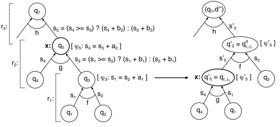
index of the counter yir that holds the reference value of the given transition, i.e., y = yir+ cr. With this notation, Figure 4 (a) shows the alternating moves of SA that simulate the A-transition considered, for one disjunct ofϕ ∧ δr. Figure 4 (b)
(c) y = 0 . . . yir y0= y − 1 . . . . . .
.qI(ir+1),fI(ir+1), (yir+1)1/
ν1 (a) . . . . . . ν2 ν3 y0= y − 1 y0= y + 1 . . . y0= y − sgn(|a|) (b) .q, a, (y)1/ .q, f , (ym)1/ y0= y + 1
.qI(ir−1),fI(ir−1), (yir−1)1/ y0= y − sgn(cr) yir+1 .q, f , (y)1/ y0= y − sgn(em) . . . . . . y = 0 y0= y + 1 y0= y + sgn(d ir−1) y0= y − sgn(dir+1) .qr,fr, (yir)1/ yir−1
Fig. 4 Simulation of a TASC by an APDS
Filled circles in Figure 4 represent states from Q × Σ, and empty circles are additional states fromΠ. The only accepting state of SA, named qf, is marked by
a double circle. The notation sgn(...) denotes the sign function, i.e., sgn(n) = 1 if n > 0, sgn(0) = 0, and sgn(n) = −1 if n < 0. Next, ν1,ν2, . . .are symbolic names
for the universal moves performed by SA. Further, in what follows, we will denote
a configuration ..q, f /,u/ of SA by writing .q, f ,u/. In particular, in Figure 4,
configurations from Q × Σ × Γ∗ are labeled by triples of the form .q, f ,(y)1/.
Here, (y)1denotes the unary encoding of the value of the y counter. Moreover, for
simplicity, configurations fromΠ ×Γ∗are labeled only with (y)1in Figure 4.
When simulating the A-transition f (q1, . . . ,qn)−→ q, Sϕ Astarts with the
config-uration .q, f ,(y)1/ (cf. Figure 4 (a)). In order to derive the reference value yirfrom y, SAperforms |cr| decrement or increment actions, depending on whether the sign
of cris positive or negative. Then SAperforms the universal moveν1making three
copies of itself (unless ir= 1 when the upper branch is omitted and/or ir= n when
the lower branch is omitted). The middle branch simply moves to the appropriate control state .qr,fr/ with stack (yir)1. The upper and lower branches are used to produce the values yir−1and yir+1if needed.
The upper branch of the universal moveν1 depicted in Figure 4 depends on
"r ∈ {≤,=}. If "r is =, then SA performs a sequence of increment/decrement
operations of length dir−1in order to obtain the value yir−1from yir(since yir−1=
yir+ dir−1). If "r is ≤, then there is an additional existential (non-deterministic)
transition—depicted using a dotted arrow in Figure 4 (a)—which decrements the counter an arbitrary number of times in order to obtain a smaller value (since yir−1≤ yir+ dir−1).
A similar sequence of transitions is performed by the lower branch ofν1. Note
that the symbols fI(ir−1),fr,fI(ir+1) are chosen arbitrarily, that is, for each triple (g1,g2,g3) ∈ Σn3, SAperforms three universal moves that are identical toν1,ν2,ν3,
with g1, g2, and g3substituted for fI(ir−1),fr, and fI(ir+1), respectively.
Next, if ir− 1 > 1, the simulation continues with the binary universal move
ν2. The lower branch of ν2 changes the control into .qI(ir−1),fI(ir−1)/ without
changing the stack. The upper branch ofν2leads to a control state fromΠ, from
which the remaining values yir−2, . . . ,y1are produced. Symmetrically, the
univer-sal moveν3leads to configurations producing the values yir+1, . . . ,yn.
Clearly, the values of the counters y1,y2, . . . ,ynthat are obtained in the way
described above will satisfy the constraintϕ ∧ δr when used as the sizes of the
subtrees tI(1),tI(2), ...,tr, ...,tI(n). Moreover, at the same time, any assignment
sat-isfying this formula can be obtained in some run of SA by iterating the
incre-ment/decrement self-loops a sufficient number of times.3
In order to simulate moves of the form a −→ q (Figure 4 (b)), SAsimply
decre-ments/increments the counter, depending on the sign of |a|, a number of times equal to the absolute value of |a|. The condition y = 0 ensures that SAaccepts only
with the empty stack. The universal dotted branch in Figure 4 (c) is used to test that ym≤ emfor some 1 ≤ m ≤ n. A similar test for yp≥ lpcan be issued by replacing
y0= y + 1 with y0= y − 1 on the loop. The following lemma is a concretisation of
the above considerations:
Lemma 5 Let A = (Q,∆,F) be a TASC over a sized alphabet (Σ,|.|) and let SA
be its corresponding APDS.
1. For any tree t ∈ T(Σ) and any run π : dom(t) → Q of A on t, there exists an accepting runρ : N∗→ (Q× Σ ∪Π) ×Γ∗of SAand an injective tree mapping
h : dom(t) → dom(ρ) between π and ρ such that:
∀p ∈ dom(t) . ρ(h(p)) = .π(p),t(p),(|t|p|)1/ (1)
2. For any accepting runρ : N∗→ (Q × Σ ∪ Π) × Γ∗of SA, there exists a tree
t ∈ T(Σ), a run π : dom(t) → Q of A on t, and an injective tree mapping h : dom(t) → dom(ρ) between π and ρ satisfying (1).
Proof (Part 1.) Let t ∈ T(Σ) be a tree and π : dom(t) → Q be a run of A on t. We prove the existence ofρ and h by induction on the structure of t.
If t = a, the only runs of A on t are generated by applying rules of the form a −→ q. In this case, for any a −→ q, ρ is the accepting run of SAstarting in .q,a,(|a|)1/
and ending with the empty stack as shown in Figure 4 (b). The tree mapping h is such that h(λ) = λ and h is undefined everywhere else. Clearly, h is an injective tree mapping (cf. Definition 1), and property (1) is satisfied.
If t = f (t1, . . . ,tn), a run of A over t has the form t ∗−→ f (q1, . . . ,qn)−→ q,ϕ
for some runs ti−→ q∗ i, 1 ≤ i ≤ n, and a transition rule f (q1, . . . ,qn)−→ q ∈ ∆ . Letϕ
1 ≤ r ≤ n be the unique integer such that |t| = |tr|+cr, and |= (ϕ ∧δr)(|t1|,...,|tn|).
3 Notice that since APDS do not have input, the universal branches are not synchronised,
By Lemma 4, there exists a permutation I ∈ Perm(n), and integers dk,em,lp∈ Z such that : n−1' k=1 |tI(k)| − |tI(k+1)| "kdk ∧ ' m∈M⊆{1,...,n} xm≤ em ∧ ' p∈P⊆{1,...,n} xp≥ lp
By the induction hypothesis, for each 1 ≤ i ≤ n, SAhas an accepting runρi
starting in a configuration .qi,ti(λ),(|ti|)1/, and there exist injective tree mappings
hi: dom(ti) → dom(ρi) satisfying property (1).
According to the construction in Figure 4 (a), SA has a run θ starting in
.q, f ,(|t|)1/ whose frontier forms a sequence p = .p1, . . . ,pn/ such that θ(pk) =
.qI(k),tI(k)(λ),(|tI(k)|)1/ for all 1 ≤ k ≤ n.
Note that for each subterm ti of the term t = f (t1, . . . ,tn), 1 ≤ i ≤ n, we can
match the control state .qi,ti(λ)/, from which the run ρiaccepting ti starts, with
the control state .qI(k),tI(k)(λ)/ at the position k = I−1(i) of the frontier ofθ. This
is due to the construction in Figure 4 (a), which produces, for each transition rule f (q1, . . . ,qn) −→ q of A, a set of runs of SA ending in control states of the form
.qi,g/ for all g ∈ Σ. It is sufficient to choose from this set the run(s) for which
gi= ti(λ) for all 1 ≤ i ≤ n.
Also, the construction in Figure 4 (a), when started with the value of the counter y being |t|, produces the values |ti| in the counters yI−1(i), 1 ≤ i ≤ n, such that |t| = |tr|+ crand |= (ϕ ∧δr)(|t1|,...,|tn|). With the above considerations, this
ensures thatθ(pk) =ρI(k)(λ) for all 1 ≤ k ≤ n.
With these definitions, the accepting runρ of SAcan be constructed asρ = θ •p
.ρI(1)(λ),...,ρI(n)(λ)/. One can see that ρ is accepting since each ρiis accepting
for all 1 ≤ i ≤ n.
The mapping h is defined such that h(λ) = λ, and for each 1 ≤ i ≤ n, for all p ∈ dom(ti), h(ip) = pI−1(i)· hi(p). The proof that h is an injective tree mapping
(cf. Definition 1) satisfying property (1) is straightforward.
(Part 2.) Letρ : N∗→ (Q × Σ ∪ Π) × Γ∗be an accepting run of SA. For an
arbitrary position p ∈ dom(ρ), let us denote by ρ↓pthe restriction ofρ to the set
{u ∈ N∗| ∀w . p ≺ w ≺ p · u ⇒ ρ(w) ∈ Π × Γ∗}. Let P = {p ∈ dom(ρ) | ρ(p) ∈
Q×Σ ×Γ∗}, and notice that ρ can be written as a composition of elementary runs
ρ↓pfor p ∈ P. We prove the existence of t, π, and h by induction on the number
N of elementary runs inρ.
For the base case N = 1, since ρ is accepting, the only possibility is that ρ is the result of simulating an existing rule a −→ q ∈ ∆ according to Figure 4 (b). Then,ρ(λ) = .q,a,γ/, and by the construction of SA, we have thatγ = (|a|)1. We
then define dom(t) = dom(π) = {λ}, t(λ) = a, and π(λ) = q. Also, let h(λ) = λ, and h be undefined everywhere else. The proof that t,π, and h satisfy property (1) is straightforward.
For the induction step N > 1, letρ↓λ be the top-most elementary run ofρ.
Letρ(λ) = .q, f,u/ be the starting configuration of ρ, and p = .p1, . . . ,pn/ be the
sequence of positions on f r(ρ↓λ), i.e.,ρ = (ρ↓λ) •p.ρ|p1, . . . ,ρ|pn/. Let ρ(pk) = .qk,fk,uk/ for all 1 ≤ k ≤ n.
By the induction hypothesis, for eachρ|pk, 1 ≤ k ≤ n, there exist trees tk, runs
πk: dom(tk) → Q of the form tk−→ q∗ k, and injective tree mappings hk: dom(tk) →
dom(ρk) satisfying property (1). Consequently, fk= tk(λ) and uk= (|tk|)1for all
1 ≤ k ≤ n.
Henceforth, we consider that n > 1, the case n = 1 being left to the reader. By the construction in Figure 4 (a), there exist:
– a transition rule f (q1, . . . ,qn)−−−−−−−−−→ q ∈ ∆ ,ϕ(x1, . . . ,xn)
– a permutation I ∈ Perm(n) such that |= ϕ(|tI−1(1)|,...,|tI−1(n)|), – a reference position 1 ≤ r ≤ n such that u = (| f (tI−1(1), . . . ,tI−1(n))|)1,
| f (tI−1(1), . . . ,tI−1(n))| = |tI−1(r)| + cr, and |= δr(|tI−1(1)|,...,|tI−1(n)|).
With these definitions, let t = f (tI−1(1), . . . ,tI−1(n)), andπ be the tree defined as
π(λ) = q, and, for all 1 ≤ i ≤ n and all p ∈ dom(πI−1(i)),π(ip) = πI−1(i)(p). It is
easy to see thatπ is a run of A over t.
The mapping h is defined such that h(λ) = λ, and for each 1 ≤ i ≤ n, for all p ∈ dom(tI−1(i)), h(ip) = pI−1(i)· hI−1(i)(p). The proof that h is an injective tree
mapping satisfying property (1) is straightforward. 12
We can now formalise the main result of this subsection.
Theorem 2 Let A be a TASC. The problem whether L(A) = /0 is decidable. Proof Due to Lemma 5, we know that a tree with a root symbol f ∈ Σ is accepted at a state q of a TASC A = (Q,∆,F) over a sized alphabet Σ iff there is an accept-ing run from the control state .q, f / in the appropriate APDS SA= (QA,Γ ,δA,FA).
It is thus enough to use the result of [4] (mentioned at the begining of the section) to check whether for some .q, f / ∈ QAwhere q ∈ F, pre∗.q, f /({.qf in,ε/}) is
non-empty. Here, qf in is the unique final state of the APDS SAconstructed according
to Figure 4. 12
Remark. The decidability of the emptiness problem for TASC can also be proved via a reduction to the class of tree automata with one memory [8] by encoding the size of a tree as a unary term. The inequality constraints from the guards of the TASC can be simulated analogously by adding increment/decrement self loops to the tree automata with one memory.
5 Semantics of Tree Updates
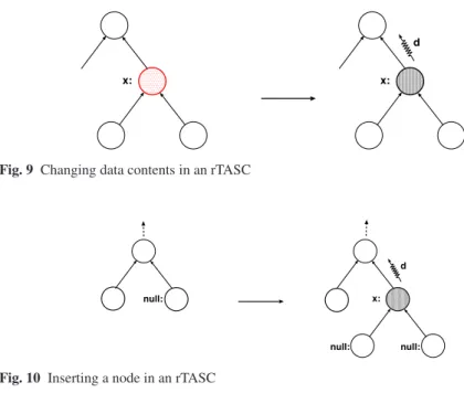
As explained in Section 2, there are three types of operations that commonly ap-pear in procedures used for balancing binary trees after an insertion or deletion: (1) navigation in a tree, i.e., testing or changing the position that a pointer vari-able is pointing to in the tree, (2) testing or changing certain data fields of the encountered tree nodes, such as the colour of a node in a red-black tree, and (3) tree rotations. In addition, one has to consider the physical insertion or deletion to/from a suitable position in the tree as an input for the re-balancing.
It turns out that the TASC defined in Section 3 are not closed with respect to the effect of some of the above operations, in particular the ones that change the balance of subtrees (the difference between the size of the left and right subtree at a given position in the tree). Therefore, we now introduce a subclass of TASC called restricted TASC (rTASC), which we show to be effectively closed with re-spect to all the needed operations on balanced trees. Moreover, rTASC are closed with respect to intersection and union, amenable to determinisation and minimisa-tion, though not closed with respect to complementation. The idea is to use rTASC to express loop invariants and pre- and post-conditions of programs as well as to perform the necessary reachability computations. TASC are then used in the asso-ciated language inclusion checks (where they arise via negation of rTASC). Remark. To simplify the presentation of the effect of program statements on a set of memory configurations given by an rTASC, we suppose in the following that the statements do not lead to a memory error (like a null pointer dereference or sim-ilar). However, it is easy to implement tests for these potential errors over sets of memory configurations described by rTASCs in the same way as regular program conditions (i.e., if statements) are implemented, which we explain in Section 5.4. 5.1 Restricted TASC
A restricted alphabet is a sized alphabet consisting only of nullary and binary symbols and a size function of the form | f (t1,t2)| = max(|t1|,|t2|) + a with a ∈ Z
for binary symbols. A restricted TASC is a TASC with a restricted alphabet and with binary rules of the form f (q1,q2) |−−−−−−−−−→ q with b ∈ Z only.1| − |2| = b
Notice that any conjunction of guards of an rTASC and their negations reduces either to false, or to only one formula of the same form, i.e., |1| −| 2| = b. Using this fact, one can show that the intersection of two rTASCs is again an rTASC, and that applying the determinisation of Section 4.1 to an rTASC yields another rTASC. Moreover, due to the fact that the guards of the transition rules of rTASCs contain at most two variables, it is not necessary to apply the potentially expensive step of converting them into the normal form described in Lemma 4, when decid-ing emptiness of rTASCs. Further, the intersection of an rTASC with a classical tree automaton is again an rTASC.4On the other hand, it is clear that rTASCs are
not closed under complementation as inequality guards are not allowed.
Minimisation of rTASC. The simple form of the guards allows us to have a prac-tical minimisation procedure based on the minimisation for classical bottom-up tree automata [9]. If (Σ,|.|) is a restricted alphabet, let Σδ be the infinite ranked
alphabet {. f ,d/ | f ∈ Σ,d ∈ Z} with #(. f ,d/) = #( f ). For any t ∈ T(Σ), let δ(t) ∈ T(Σδ) be the tree defined as follows:
– dom(t) = dom(δ(t)),
– for all p ∈ dom(t), if #(t(p)) = 0, we have δ(t)(p) = .t(p),|t(p)|/, and – for all p ∈ dom(t), if #(t(p)) = 2, we have δ(t)(p) = .t(p),|t|p1| − |t|p2|/.
In other words, we record the balance of each subtree in the symbol that labels the root of the subtree. For constant symbols, we simply put their measures as labels in the tree. Obviously,δ is a (bijective) function from T(Σ) to T(Σδ), which we
extend pointwise to sets of trees. If A is an rTASC over the restricted alphabet (Σ,|.|), let Aδbe the bottom-up tree automaton overΣδ defined by replacing each
transition rule of A of the form: – a −→ q by .a,|a|/ −→ q, and
– f (q1,q2) |−−−−−−−−−→ q by . f ,b/(q1| − |2| = b 1,q2) −→ q.
Note that we can always define Aδ over a finite subset ofΣδsince the number of
rules in A is finite. Moreover, the size of A (number of states) equals the size of Aδ. Last, the transformation of A into Aδ is always reversible.
Lemma 6 Given an rTASC A over a sized alphabet (Σ,|.|), for all trees t ∈ T(Σ), we have t ∈ L (A) if and only if δ(t) ∈ L (Aδ).
Proof We prove that t ∗−→
A q iffδ(t) ∗−−→Aδ q by induction on the structure of t. If t =
a ∈ Σ0, a −→
A q if and only ifδ(a) = .a,|a|/ −−→Aδ q. Otherwise, let t = f (t1,t2) ∗−→A f (q1,q2) |−−−−−−−−−→1| − |2| = b
A q with ti
∗ −→
A qi, 1 ≤ i ≤ 2. Then, |t1|−|t2| = b, hence δ (t) = . f ,b/(δ (t1),δ(t2)). By the induction hypothesis, we haveδ(ti) ∗−−→
Aδ qi, and, by the definition of Aδ, . f ,b/(q1,q2) −−→
Aδ q. The other direction is symmetrical. 12
Now, given an rTASC A, we compute Aδ, determinise and minimise it us-ing the classical construction from [9], obtainus-ing Aδmin. The minimal rTASC
Amin is subsequently obtained by performing a reverse of the conversion from
rTASC to tree automata on Aδmin, i.e., by moving back the integer constants
from the symbols to the guards. To convince ourselves that Aminis indeed
min-imal, suppose there exists a smaller rTASC A0recognising the same language, i.e.,
L (A) = L (Amin) = L (A0). Then,δ(L (A)) = δ(L (A0)) = L (A0δ) = L (Aδmin).
Since A0and A0
δ have the same number of states, we contradict the minimality of
Aδmin.
5.2 Representing Sets of Memory Configurations
To be able to describe how tree rotations (and the other considered operations) can be implemented over rTASC, we first have to explain how rTASC can be used for describing sets of memory configurations of programs manipulating balanced tree structures like red-black trees or AVL trees. Intuitively, we map memory config-urations (i.e., heap graphs) having the form of trees node-by-node onto the trees accepted by rTASC, with the nodes labelled by (1) the variables pointing to them and by (2) the data elements stored in them. We also use the label null to denote null successors of leaf nodes.
Formally, let us consider a finite set of pointer variables V = {x,y,...} and a finite set of data values D, e.g., D = {red,black}. In the following, we let Σ = P(V )× D ∪ {null}. The arity function is defined as follows: #( f ) = 2 for all f ∈ P(V ) × D, and #(null) = 0. For any non-null symbol f ∈ P(V ) × D, let v( f ) ⊆ V and d( f ) ∈ D denote the variables pointing to the tree node labelled with f and the data value of this node, respectivelly, i.e., f = (v( f ),d( f )). For a tree t ∈ T(Σ) and a variable x ∈ V , we say that a node p ∈ dom(t) is pointed to by x if and only if t(p) '= null and x ∈ v(t(p)). If there is no node pointed by a variable x ∈ V in a tree t ∈ T(Σ), i.e., ∀p ∈ dom(t). t(p) '= null ⇒ x '∈ v(t(p)), we assume x to be null.5
For the rest of the section, let A = (Q,∆,F) be an rTASC over Σ. We say that A represents a set of memory configurations if and only if for each t ∈ L(A) and each x ∈ V , there is at most one p ∈ dom(t) that is pointed to by x. This condition can be always enforced by intersecting any given rTASC by the rTASC A0= (Q0,∆0,Q0) where Q0= P(V ), and ∆0= {null −→ /0} ∪{ f (v1,v2)−→ v |5
v = v( f )∪v1∪v2∧ v( f )∩v1= v( f )∩v2= v1∩v2= /0}. Intuitively, A0remembers
in its control locations all so-far encountered variables and ensures that no variable is encountered twice.
An example of an rTASC representing within the described encoding the set of memory configurations correponding to the invariant in the red-black tree in-sertion procedure can be found at the beginning of Section 6.
5.3 Computing the Effect of Tree Rotations
Let x ∈ V be a fixed variable, and A = (Q,∆,F) be an rTASC. We now give a method for deriving an rTASC A0= (Q0,∆0,F0) describing the set of trees that
are the result of a left rotation applied to trees from L(A) at the node pointed to by x. The case of the right tree rotation is very similar and so we skip it here.6In the
description, we will be referring to Figure 5 illustrating the problem.
Let Rx(∆) = {(r1,r2) ∈ ∆ ×∆ | r1: f (q1,q2)−−→ qϕ3 3 ∧ r2: g(q4,q3)−−→ qϕ5 5∧
x ∈ v(g)} be the set of all the pairs of automata rules from ∆ that can yield a ro-tation, and be modified because of it. Other rules may then have to be modified to reflect:
– changes of some control states, for instance the change of q5to q03in rule r3
from Figure 5, or
– changes of balance resulting from the rotation, i.e., changes in the difference between the sizes of left and right subtrees, which get propagated from the rotated subtree upwards.
To define the resulting automaton, we use an auxiliary set D ⊆ Z which con-tains all the changes in balance that may occur in any tree from L(A), due to a rotation at x. The set D is the smallest set such that:
5 For simplicity, we do not explicitly distinguish null and undefined pointer values. Such a
distinction could, however, be easily introduced.
6 In fact, it can be implemented by temporarily swapping the child nodes in the involved rules,
q1 q2 q3 q4 q5 s1 s2 s3 = (s1 >= s2) ? (s1 + b1) : (s2 + b1) s4 f g [ $3: s1 = s2 + a1 ] [ $5: s4 = s3 + a2 ] s5 = (s4 >= s3) ? (s4 + b2) : (s3 + b2) q4 q1 s4 s1 g q2 s’5 f s2 s’3 [ $’3 ] [ $’5 ] r1: r2: h q7 h (q7,d’’) x: q’3 = q d r1,r2 q’5 = qr1,r2 x: r3:
Fig. 5 Left rotation on an rTASC
– iniD(r1,r2) ∈ D, for all (r1,r2) ∈ Rx, and
– le ftD(a,d) ∈ D, rightD(a,d) ∈ D, for all d ∈ D and f (q1,q2) |−−−−−−−−−→1| = |2| + a
q3∈ ∆ .
The function iniD computes the initial disbalance caused by the rotation, while le f tD and rightD propagate upward the disbalance that happened in the left or right subtree of some node, respectivelly. The definitions of these functions are the subject of Sections 5.3.1 and 5.3.2. Lemma 7 shows that the set D is finite, which guarantees that A0can be computed in a finite number of steps.
The set of states of A0is defined as Q0= Q ∪Qx∪ QD
x ∪ QD, where Qx,QDx and
QDare pairwise disjoint sets, all disjoint from Q, defined as:
– Qx= {qr1,r2| (r1,r2) ∈ Rx(∆)} contains a new state for each pair of transition
rules involved in the rotation, which accepts the former root of the rotated subtree that went down in the rotation.
– QD
x = {qdx | qx∈ Qx ∧ d ∈ D} is the set of states accepting the nodes that went
up in the rotation and became the new root of the rotated subtree.
– QD = {qd| q ∈ Q ∧ d ∈ D} is the set of states accepting all contexts of
subtrees changed by the rotation (i.e., the tree nodes that appear above the rotated subtree).
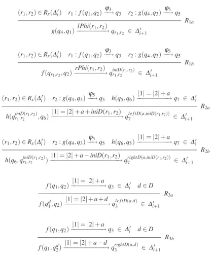
The set∆0 of transition rules of A0 is defined as the limit of the increasing
sequence of sets∆0
0⊆ ∆10 ⊆ ∆20, . . ., i.e.,∆0=(i≥0∆i0, where∆00=∆, and ∆i+10 is
obtained from∆0
i by applying one of the rules in Figure 6. Since, by Lemma 7,
the set D is finite, it is obvious that the limit is reached in a finite number of steps. The functions lPhi and rPhi that compute the guards of the newly added rules, are given in Section 5.3.1.
The set of final states of A0is defined as F0= {qd
| q ∈ F} ∪{ qdr1,r2| (r1,r2) ∈ Rx ∧ d = iniD(r1,r2) ∧ r1: f (q1,q2)−−→ qϕ3 3 ∧ r2: g(q4,q3)−−→ qϕ5 5 ∧ q5∈ F}.
Intuitivelly, the states from {qd | q ∈ F} ensure that we accept only the trees in
which a rotation actually occurred in some subtree. Additionaly, the states qd r1,r2∈
(r1,r2) ∈ Rx(∆i0) r1: f (q1,q2)−−→ qϕ3 3 r2: g(q4,q3)−−→ qϕ5 5 g(q4,q1)−−−−−−−−→ qlPhi(r1,r2) r1,r2 ∈ ∆i+10 R1a (r1,r2) ∈ Rx(∆i0) r1: f (q1,q2)−−→ qϕ3 3 r2: g(q4,q3)−−→ qϕ5 5 f (qr1,r2,q2) rPhi(r1,r2) −−−−−−−−→ qiniD(r1,r2) r1,r2 ∈ ∆i+10 R1b (r1,r2) ∈ Rx(∆i0) r2: g(q4,q3)−−→ qϕ5 5 h(q5,q6) |−−−−−−−−−→ q1| = |2| + a 7 ∈ ∆i0 h(qiniD(r1,r2) r1,r2 ,q6) | 1| = |2| + a + iniD(r1,r2) −−−−−−−−−−−−−−−−−−−→ qle ftD(a,iniD(r1,r2)) 7 ∈ ∆i+10 R2a (r1,r2) ∈ Rx(∆i0) r2: g(q4,q3)−−→ qϕ5 5 h(q6,q5) |−−−−−−−−−→ q1| = |2| + a 7 ∈ ∆i0 h(q6,qiniD(rr1,r2 1,r2)) | 1| = |2| + a − iniD(r1,r2) −−−−−−−−−−−−−−−−−−−→ qrightD(a,iniD(r1,r2)) 7 ∈ ∆i+10 R2b f (q1,q2) |−−−−−−−−−→ q1| = |2| + a 3 ∈ ∆i0 d ∈ D f (qd 1,q2) |−−−−−−−−−−−→ q1| = |2| + a + d le ftD(a,d)3 ∈ ∆i+10 R3a f (q1,q2) |−−−−−−−−−→ q1| = |2| + a 3 ∈ ∆i0 d ∈ D f (q1,qd2) |−−−−−−−−−−−→ q1| = |2| + a − d rightD(a,d)3 ∈ ∆i+10 R3b
Fig. 6 Rules for computing the effect of left rotations on rTASCs
F0, accepting the root of the rotated subtree, become final if the rotation occurs at
a state q5accepting the root node of the original tree (i.e., if q5∈ F).
5.3.1 The Root of the Rotated Subtree: Computing lPhi, rPhi, and iniD
Let us consider (r1,r2) ∈ Rx(∆) where r1: f (q1,q2)−→ qϕ3 3and r2: g(q4,q3)−→ϕ5
q5, as in Figure 5. Suppose thatϕ3: |1| = |2| + a1and let us denote the sizes of
the subtrees read at q1and q2before the rotation, by s1and s2, respectively. Let
the size function associated with f be | f (t1,t2)| = max(|t1|,|t2|) + b1, and let s3
denote the size of the subtree labelled by q3 before the rotation. Also, suppose
thatϕ5: |1| = |2| + a2and let us denote the size of the sub-tree read at q4before
the rotation as s4. Finally, let the size function associated with g be |g(t1,t2)| =
max(|t1|,|t2|) + b2, and let s5denote the size of the subtree labelled by q5before
the rotation. We denote s0
The key observation that allows us to compute the guardsϕ0
5: lPhi(r1,r2) and
ϕ0
3: rPhi(r1,r2) of the rules that accept the root of the rotated subtree, as well as
the change in balance d = iniD(r1,r2) caused by the rotation, is that due to the
chosen form of guards and sizes, we can always compute any two of the sizes s1,
s2, s4from the remaining one. Indeed,
– for a1≥ 0, we have s3= s1+ b1= s2+ a1+ b1= s4− a2, whereas
– for a1<0, we have s3= s2+ b1= s1− a1+ b1= s4− a2.
Computingϕ0
3,ϕ50, and d is then just a complex exercise in case splitting. Notice
that all the cases can be distinguished statically according to the mutual relations of the constants a1, b1, a2, and b2. In the case ofϕ50, we obtain the following:
1. For a1≥ 0, we have s4= s1+ b1+ a2, and soϕ50 : |1| = |2| + b1+ a2.
2. For a1<0, we have s4= s1− a1+b1+a2, and soϕ50: |1| = |2|−a1+b1+a2.
The guardϕ0
3is a bit more complex. We distinguish two cases:Φ4≥1: s4≥ s1
andΦ4<1: s4<s1. Now we rewrite the conditions s4≥ s1and s4<s1using the
relation between s4and s1described above for a1≥ 0 and a1<0:
1. Φ4≥1: s4≥ s1 ⇐⇒ (a1≥ 0 ∧ b1+ a2≥ 0) ∨ (a1<0 ∧−a1+ b1+ a2≥ 0). If
Φ4≥1holds, then s0
5= s4+ b2. Further, we distinguish between the following
cases:
(a) For a1≥ 0 ∧ b1+ a2≥ 0, we get s05= s1+ b1+ a2+ b2(as a1≥ 0), i.e.,
s1= s05− b1− a2− b2. Taking into account that s1= s2+ a1, we obtain
ϕ0
3: |1| = |2| + a1+ b1+ a2+ b2.
(b) For a1<0 ∧ −a1+ b1+ a2≥ 0, we have s50 = s1− a1+ b1+ a2+ b2(as
a1<0), i.e., s1= s05+a1− b1− a2− b2. Using that s1= s2+a1, we obtain
ϕ0
3: |1| = |2| + b1+ a2+ b2.
2. Φ4<1: s4<s1 ⇐⇒ (a1≥ 0 ∧ b1+ a2<0) ∨(a1<0 ∧−a1+ b1+ a2<0). If
Φ4<1holds, we have s05= s1+ b2, and soϕ30 : |1| = |2| + a1+ b2.
The computation of the change in the balance d is similar to the above. The first case to be considered isΦ4≥3: s4≥ s3 ⇐⇒ a2≥ 0. Here, s5= s4+b2. To compute
the change in the sizes reached at q5and q03, which is to be compensated in the
transitions to come after q0
3instead of q5, we need to compute s03as a function of
s4(then, in the difference, s4will be eliminated). We can write the following:
s0 3= if&Φ4≥1: if s4+ b2≥ s2: s4+ b2+ b1 if s4+ b2<s2: s2+ b1 if&Φ4<1: if s1+ b2≥ s2: s1+ b2+ b1 if s1+ b2<s2 : s2+ b1
Let us first consider the subcase whenΦ4≥1. It has two further subcases s4+
b2≥ s2and s4+b2<s2, which we can again rewrite by using the known relations
between s4and s2for a1≥ 0 (s2+a1+b1= s4−a2) and a1<0 (s2+b1= s4−a2).
We get:
1. s4+b2≥ s2⇐⇒ (a1≥ 0 ∧ a1+b1+a2+b2≥ 0) ∨ (a1<0 ∧ b1+a2+b2≥
0). In this case, we have s0
q1 q2 q3 s1 s2 s3 = (s1 >= s2) ? (s1 + b) : (s2 + b) f [ $: s1 = s2 + a ] d d’ q2 s’1 s2 s’3 = (s’1 >= s2) ? (s’1 + b) : (s2 + b) f [ $’: s’1 = s2 + a + d ] q1 q2 q3 s1 s2 s3 = (s1 >= s2) ? (s1 + b) : (s2 + b) f [ $: s1 = s2 + a ] d d’’ q1 s1 s’2 s’’3 = (s1 >= s’2) ? (s1 + b) : (s’2 + b) f [ $’’: s1 = s’2 + a - d ] qd 2 qd’’ 3 (a) (b) qd 1 qd’ 3
Fig. 7 Propagation of changes in balance in an rTASC
2. s4+b2<s2⇐⇒ (a1≥ 0 ∧ a1+b1+a2+b2<0) ∨ (a1<0 ∧ b1+a2+b2<
0). Here, s0
3= s2+ b1, and we distinguish the following subcases:
(a) for a1≥ 0 ∧ a1+b1+a2+b2<0, s03= s2+b1= s4− a1− b1− a2+b1=
s4− a1− a2, and so d = −a1− a2− b2.
(b) for a1<0 ∧ b1+ a2+ b2<0, s03= s2+ b1= s4− b1− a2+ b1= s4− a2,
and so d = −a2− b2.
The remaining cases of the computation of d are similar to the above.
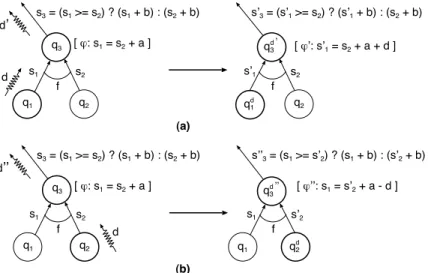
5.3.2 Propagating Changes in Balance through rTASC: Computing le f tD, rightD We now study the way how a change in balance caused by a rotation is propagated from the subtree where the rotation took place to the root of the entire tree in which the rotation happened. The propagation is a part of the rules (R2a)–(R3b) from Figure 6, and it is illustrated in Figure 7 on a rule f (q1,q2)−→ qϕ 3whose
left or right child size changes by a value d ∈ D. Consequently, rules of the form f (qd
1,q2) ϕ 0
−→ qd30 or f (q1,qd2) ϕ 00
−−→ qd300 are generated by the rules (R2a)–(R3b),
depending on whether the change in balance originates from the left or the right. Since we consider just one rotation in every tree (at a given node pointed to by the pointer variable x), the change can never come from both sides. The guards of the new rules, compensating the change in balance that happens between the child nodes, areϕ0: |1| = |2| + a + d or ϕ00: |1| = |2| + a − d, respectivelly. It remains
to analyse the changes in the balance that are propagated upwards after d comes from the bottom, i.e., the way the values d0= le f tD(a,d) or d00= rightD(a,d) are
computed.
Suppose the change in balance is coming from the left as in Figure 7 (a). We distinguish the cases of a ≥ 0 and a < 0. (1) For a ≥ 0, the original size at q3is