HAL Id: inria-00526993
https://hal.inria.fr/inria-00526993
Submitted on 17 Oct 2010
HAL is a multi-disciplinary open access
archive for the deposit and dissemination of
sci-entific research documents, whether they are
pub-lished or not. The documents may come from
teaching and research institutions in France or
abroad, or from public or private research centers.
L’archive ouverte pluridisciplinaire HAL, est
destinée au dépôt et à la diffusion de documents
scientifiques de niveau recherche, publiés ou non,
émanant des établissements d’enseignement et de
recherche français ou étrangers, des laboratoires
publics ou privés.
Salim Jouili, Salvatore Tabbone
To cite this version:
Salim Jouili, Salvatore Tabbone. Graph Embedding Using Constant Shift Embedding. D. Ünay,
Z. Cataltepe, and S. Aksoy. International Conference on Pattern Recognition - ICPR 2010, 6388,
Springer Berlin / Heidelberg, pp.83-92, 2010, Lecture Notes in Computer Science. �inria-00526993�
Embedding
⋆Salim Jouili and Salvatore Tabbone
LORIA - INRIA Nancy Grand Est UMR 7503 - University of Nancy 2 BP 239, 54506 Vandoeuvre-l`es-Nancy Cedex, France
{salim.jouili,tabbone}@loria.fr
Abstract. In the literature, although structural representations (e.g. graph) are more powerful than feature vectors in terms of represen-tational abilities, many robust and efficient methods for classification (unsupervised and supervised) have been developed for feature vector representations. In this paper, we propose a graph embedding technique based on the constant shift embedding which transforms a graph to a real vector. This technique gives the abilities to perform the graph clas-sification tasks by procedures based on feature vectors. Through a set of experiments we show that the proposed technique outperforms the clas-sification in the original graph domain and the other graph embedding techniques.
Key words: Structural pattern recognition, graph embedding, graph classification
1
Introduction
In pattern recognition, object representations can be broadly divided into sta-tistical and structural methods [1]. In the former, the object is represented by a feature vector, and in the latter, a data structure (e.g. graphs or trees) is used to describe the components and their relationships into the object. In the lit-erature, many robust and efficient methods for classification (unsupervised and supervised), retrieval and other related tasks are henceforth available [5]. Most of these approaches are often limited to work with a statistical representation. Indeed, the use of feature vectors has numerous helpful properties. That is, since recognition is to be carried out based on a number of measurements of the ob-jects, and each feature vector can be regarded as a point in an n-dimensional space, the measurement operations can be performed in simple way such that the Euclidean distance as the distance between objects. When a numerical feature vector is used to represent the object, all structural information is discarded. However a structural representation (e.g. graph) is more powerful than feature
⋆
This work is partially supported by the French National Research Agency project NAVIDOMASS referenced under ANR-06-MCDA-012 and Lorraine region. For more details and resources see http://navidomass.univ-lr.fr
vector in terms of representational abilities. The graph structure provides a flex-ible representation such that there is no fixed dimensionality for objects (unlike vectors), and provides an efficient representation such that an object is modeled by its components and the existing relations between them. In the last decades, many structural approaches have been proposed [3]. Nevertheless, dealing with graphs suffers, on the one hand from the high complexity of the graph match-ing problem which is a problem of computmatch-ing distances between graphs, and on the other hand from the robustness to structural noise which is a problem related to the capability to cope with structural variation. These drawbacks have brought about a lack of suitable methods for classification. However, unlike for structural-based representation, a lot of robust classification approaches have been developed for the feature vector representation such as neural network, sup-port vector machines, k-nearest neighbors, Gaussian mixture model, Gaussian, naive Bayes, decision tree and RBF classifiers [12]. In contrast, as remarked by Riesen et al. [2] the classification of graphs is limited to the use of the nearest-neighbor classifiers using one graph similarity measure. On that account, the community of pattern recognition speaks about a gap between structural and statistical approaches [1, 16].
Recently, a few works have been carried out concerning the bridging of this gap between structural and statistical approaches. Their aim is to delineate a mapping between graphs and real vectors, this task is called graph embedding. The embedding techniques were originally introduced for statistical approaches with the objective of constructing low dimensional feature-space embeddings of high-dimensional data sets [6, 9, 17, 22]. In the context of graph embedding, different procedures have been proposed in the literature. De Mauro et al. [4] propose a new method, based on recurrent neural network, to project graphs into vector space. Moreover, Hancock et al. [7, 27, 14, 21] use spectral theory to convert graphs into vectors by means of spectral decomposition into eigenvalues and eigenvectors of the adjacency (or Laplacian) matrix of a graph. Besides, a new category of graph embedding techniques was introduced by Bunke et al. [2, 20, 19], their method is based on the selection of some prototypes and the computation of the graph edit distance between the graph and the set of prototypes. This method was originally developed for the embedding of feature vectors in a dissimilarity space [16, 17]. This technique was also used to project string representations into vector spaces [25].
In this paper, we propose a new graph embedding technique by means of constant shift embedding. Originally, this idea was proposed in order to pairwise data into Euclidean vector spaces [22]. It was used to embed protein sequences into an n-dimensional feature vector space. In the current work, we generalize this method to the domain of graphs. Here, the key issue is to convert general dissimilarity data into metric data. The constant shift embedding increases all dissimilarities by an equal amount to produce a set of Euclidean distances. This set of distances can be realized as the pairwise distances among a set of points in an Euclidean space. In our method, we generalize this method by means of graph similarity measure [11, 10]. The experimental results have shown that the
pro-posed graph embedding technique improves the accuracy achieved in the graph domain by the nearest neighbor classifier. Furthermore, the results achieved by our method outperforms some alternative graph embedding techniques.
2
Graph similarity measure by means of node signatures
Before introducing the graph embedding approach, let us recall how the dissim-ilarity in the domain of graphs can be computed. Simdissim-ilarity or (dissimdissim-ilarity) between two graphs is almost always refered as a graph matching problem. Graph matching is the process of finding a correspondence between nodes and edges of two graphs that satisfies some constraints ensuring that similar substructures in one graph are mapped to similar substructures in the other. Many approaches have been proposed to solve the graph matching problem. In this paper we use a recent technique proposed by Jouili et al. in [10, 11]. This approach is based on node signatures notion. In order to construct a signature for a node in an attributed graph, all available information into the graph and related to this node is used. The collection of these informations should be refined into an ade-quate structure which can provides distances between different node signatures. In this perspective, the node signature is defined as a set composed by four sub-sets which represent the node attribute, the node degree and the attributes of its adjacent edges and the degrees of the nodes on which these edges are connected. Given a graph G=(V,E,α,β), the node signature of ni∈ V is defined as follows:
γ(ni) =
n
αi, θ(ni), {θ(nj)}∀ij∈E, {βij}∀ij∈E
o
where
– αi the attribute of the node ni.
– θ(ni) the degree of ni.
– {θ(nj)}∀ij∈Ethe degrees set of the nodes adjacent to ni.
– {βij}∀ij∈E the attributes set of the incident edges to ni.
Then, to compute a distance between node signatures, the Heterogeneous Euclidean Overlap Metric (HEOM) is used. The HEOM uses the overlap met-ric for symbolic attributes and the normalized Euclidean distance for numemet-ric attributes. Next the similarities between the graphs is computed: Firstly, a defi-nition of the distance between two sets of node signatures is given. Subsequently, a matching distance between two graphs is defined based on the node signatures sets. Let Sγ be a collection of local descriptions, the set of node signatures Sγ of
a graph g=(V,E,α,β) is defined as : Sγ( g ) =
n
γ(ni) | ∀ni∈ V
o
Let A=(Va,Ea) and B=(Vb,Eb) be two graphs. And assume that φ : Sγ(A) →
distance between Sγ(A) and Sγ(B)
d(A, B) = ϕ(Sγ(A), Sγ(B)) = min φ
X
γ(ni)∈Sγ(A)
dnd(γ(ni), φ(γ(ni)))
The calculation of the function ϕ(Sγ(A), Sγ(B)) is equivalent to solve an
as-signment problem, which is one of the fundamental combinatorial optimization problems. It consists of finding a maximum weight matching in a weighted bi-partite graph. This assignment problem can be solved by the Hungarian method. The permutation matrix P, obtained by applying the Hungarian method to the cost matrix, defines the optimum matching between two given graphs.
3
Graph embedding via constant shift embedding
Embedding graph corresponds to finding points in a vector space, such that their mutual distance is as close as possible to the initial dissimilarity matrix with respect to some cost function. Embedding yields points in a vector space, thus making the graph available to numerous machine learning techniques which require vectorial input.
Let G={g1, ..., gn} be a set of graph and d: G × G → R a graph distance
function between pairs of its elements and let D = Dij = d(gi, gj) ∈ Rn×n be
an n × n dissimilarity matrix. Here, the aim is to yield n vectors xi in a
p-dimensional vector space such that the distance between xi and xj is close to
the dissimilarity Dij which is the distance between gi and gj.
3.1 Dissimilarity Matrix: from Graph domain to Euclidean space via Constant shift embedding
Before stating the main method, the notion of centralized matrix is reminded [22]. Let P be an n × n matrix and let In be the n × n identity matrix and
en=(1,...,1)⊺. Let Qn =In
-1 nene
⊺
n. Qn is the projection matrix onto the
orthog-onal complement of en. The centralized matrix Pc is given by:
Pc= QnP Qn
Roth et al. [22] observed that the transition from the original matrix D (in our case: the graph domain) to a matrix ˜D which derives from a squared Euclidean distance, can be achieved by a off-diagonal shift operation without influencing the distribution of the initial data. Hence, ˜D is given by:
˜
D = D + d0(ene⊺n− In), or similarly ( ˜Dij= Dij+ d0,∀i 6= j)
Where d0 is constant. In addition, since D is a symmetric and zero-diagonal
matrix, it can be decomposed [13] by means of a matrix S: Dij = Sii+ Sjj− 2Sij
Obviously, S is not uniquely determined by D. All matrices S + αene⊺n yield
the same D, ∀α ∈ R. However, it is proven that the centralized version of S is uniquely defined by the given matrix D (Lemma 1 in [22]):
Sc = −1 2D
c, with Dc= Q nDQn
From the following important theorem [26], we remark the particularity of the interesting matrix Sc.
Theorem 1. D is squared Euclidean distance matrix if and only if Sc is
positive and semidefinite.
In other words, the pairwise similarities given by D can be embedded into an Euclidean vector space if and only if the associated matrix Scis positive and
semidefinite. As far as graph domain, Sc will be indefinite. We use the constant
shift embedding [22] to cope this problem. Indeed, by shifting the diagonal el-ements of Sc it can be transformed into a positive semidefinite matrix ˜S (see
Lemma 2. in [22]):
˜
S = Sc− λ n(Sc)In
where λn(Sc) is the minimal eigenvalue of the matrix Sc. The diagonal shift of
the matrix Sc transforms the dissimilarity matrix D in a matrix representing
squared Euclidean distances. The resulting embedding of D is defined by: ˜
Dij = ˜Sii + ˜Sjj - 2˜Sij⇐⇒ ˜D = D − 2λn(Sc)(ene⊺n− In)
Since every positive and semidefinite matrix can be thought as representing a dot product matrix, there exists a matrix X for which ˜Sc = XX⊺. The rows of
X are the resulting embedding vectors xi, so each graph gi has been embedded
in a Euclidean space and is represented by xi. Then, it can be concluded that
the matrix ˜D contains the squared Euclidean distances between these vectors xi. In the next section, we discuss the extension of this method to the graph
embedding.
3.2 From graphs to vectors
In this section, an algorithm for constructing embedded vectors is described. This algorithm is inspired from the Principal Component Analysis (PCA) [23]. A pseudo-code description of the algorithm is given in Algorithm 1. From a given dissimilarity matrix D of a set of graphs G={g1, ..., gn}, the algorithm returns
a set of embedded vectors X={x1,· · · , xn} such that xi embed the graph gi.
Firstly, the squared Euclidean distances matrix ˜D is computed by means of the constant shift embedding (line 1). Next, the matrix ˜Sc is computed, and as
stated above it can be calculated as ˜Sc= −1
2D˜
c (line 2). Since ˜Sc is positive and
semidefinite matrix, thus, ˜Sc=XX⊺. The rows of X are the resulting embedding
vectors xi and they will be recovered by means of an eigendecomposition (line
3). Let note that, due to the centralization, it exists at least one the eigenvalue λi=0, hence, p ≤ n − 1 (line 3-4). Finally by computing the n × p map matrix:
Xp=Vp(Λp)1/2, the embedded vectors are given by the rows of X = Xp, in
p-dimensional space.
However, in PCA it is known that small eigenvalues contain the noise. There-fore, the dimensionality p can reduced by choosing t ≤ p in line 4 of the algo-rithm. Consequently, a n× t map matrix Xt=Vt(Λt)1/2will be computed instead
of Xp, where Vtis the column-matrix of the selected eigenvectors (the first t
col-umn vectors of V) and Λtthe diagonal matrix of the corresponding eigenvectors
(the top t × t sub-matrix of Λ). One can ask how to find the optimal t that yields the better performance of a classifier in the vector space. Indeed, the dimension-ality t has a pronounced influence on the performance of the classifier. In this paper, the optimal t is chosen empirically. That means, the optimal t is the one which provides the better classification accuracy from 2 to p.
Algorithm 1Construction of the embedded vectors
Require: Dissimilarity matrix D of the a set of graphs G={g1, ..., gn}
Ensure: set of vectors X={x1,· · · , xn} where xiembed gi
1: Compute the squared Euclidean distances matrix ˜D
2: ⊲ ˜D = D − 2λn(Sc)(ene⊺n− In) 3: ⊲ Sc= −1 2D c, with Dc= Q nDQn 4: ⊲Qn=In-1 nene ⊺
n, with Inthe n × n identity matrix and en=(1,...,1)⊺.
5:
6: Compute ˜Sc= −1
2 D˜
c, where ˜Dc= Q ˜DQ.
7: Eigendecomposition of ˜Sc, ˜Sc= V ΛV⊺
– Λ=diag(λ1, ...λn) is the diagonal matrix of the eigenvalues
– V={υ1, ...υn} is the orthonormal matrix of corresponding eigenvectors υi.
⊲Note that, λ1≥ ... λp≥ λp+1= 0 = ... = λn
8: Compute the n × p map matrix: Xp=Vp(Λp)1/2, with Vp={υ1, ...υp} and Λp=
diag(λ1, ...λp)
9: Output: The rows of Xp contain the embedded vectors in p-dimensional space.
4
Experiments
4.1 Experimental setup
To perform the evaluation of the proposed algorithm, we used four data sets : – GREC: The GREC data set [18] consists of graphs representing symbols
from architectural and electronic drawings. Here, the ending points (i.e. cor-ners, intersections and circles) are represented by nodes which are connected by undirected edges and labeled as lines or arcs. The graph subset used in our experiments has 814 graphs, 24 classes and 37 graphs per class.
Algorithm 2Construction of the embedded vectors
Require: Dissimilarity matrix D of the a set of graphs G={g1, ..., gn}
Ensure: set of vectors X={x1,· · · , xn} where xiembed gi
1: Compute the squared Euclidean distances matrix ˜D 2: Compute ˜Sc= −1
2 D˜
c, where ˜Dc= Q ˜DQ.
3: Eigendecomposition of ˜Sc, ˜Sc= V ΛV⊺
– Λ=diag(λ1, ...λn) is the diagonal matrix of the eigenvalues
– V={υ1, ...υn} is the orthonormal matrix of corresponding eigenvectors υi.
⊲Note that, λ1≥ ... λp≥ λp+1= 0 = ... = λn
4: Compute the n × p map matrix: Xp=Vp(Λp)1/2, with Vp={υ1, ...υp} and Λp=
diag(λ1, ...λp)
5: Output: The rows of Xp contain the embedded vectors in p-dimensional space.
– Letter: The Letter data set [18] consists of graphs representing distorted Letter drawings. This data set contains 15 capital letters (A, E, F, H, I, K, L, M, N, T, V, W, X, Y, Z), arbitrarily strong distortions are applied to each letter to obtain large sample sets of graphs. Here, the ending points are represented by nodes which are connected by undirected edges. The graph subset used in our experiments has 1500 graphs, 15 classes and 100 graphs per class.
– COIL: The COIL data set [15] consists of graphs representing different views of 3D objects in which two consecutive images in the same class represent the same object rotated by 5o. The images are converted into graphs by
feature points extraction using the Harris interest points [8] and Delaunay triangulation. Each node is labeled with a two-dimensional attribute giv-ing its position, while edges are unlabeled. The graph subset used in our experiments has 2400 graphs, 100 classes and 24 graphs per class.
– Mutagenicity: The Mutagenicity data set [18] consists of graphs represent-ing molecular compounds, the nodes represent the atoms labeled with the corresponding chemical symbol and edges by valence of linkage. The graph subset used in our experiments has 1500 graphs, 2 classes and 750 graphs per class.
The experiments consist in applying our algorithm for each dataset. Our in-tention is to show that the proposed graph embedding technique is indeed able to yield embedded vectors that can improve classification results achieved with the original graph representation. We begin by computing the dissimilarities matrix of each data set by means of the graph matching introduced in [10, 11] and briefly reviewed in Section 2. Then, since the classification in the graph domain can be performed by only the k-NN classifiers, hence, it is used as reference system in the graph domain. Whereas in vector space the k-NN and the SVM1 classifiers
[24] are used to compare the embedding quality of the vectors resulting from our algorithm and the vectors resulting from the graph embedding approach
1
We used the C-SVM classifier with linear kernel function available in weka software http://www.cs.waikato.ac.nz/ml/weka/
recently proposed by Bunke et al. [2, 19, 20]. This method was originally devel-oped for the embedding of feature vectors in a dissimilarity space [16, 17] and is based on the selection of some prototypes and the computation of the graph edit distance between the graph and the set of prototypes. That is, let assume that G={g1, ..., gn} is a set of graphs and d: G × G → R is some graph
dis-similarity measure. Let P S={ps1, ..., psp} be a set of p ≤ n selected prototypes
from G (P S ⊆ G). Now each graph g ∈ G can be embedded into p-dimensional vector (d1, ..., dp), where d1 = d(g, ps1), ..., dp = d(g, psp). As remarked in [20],
the results of this method depends on the choice of p appropriate prototypes. In this paper, four different prototype selector are used, namely, the k-centers prototype selector (KCPS), the spanning prototype selector (SPS), the target-sphere prototype selector (TPS) and the random prototype selector (RandPS). We refer the reader to [20] for a definition of these selectors. A second key issue of this method is the number p of prototypes that must be selected to obtain the better classification performance. To overcome this problem, we define the optimal p by the same procedure that is applied to determine the optimal t of our algorithm (cf. section 3.2).
4.2 Results
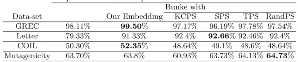
Graph domain Vector space
Bunke with
Data-set Our Embedding KCPS SPS TPS RandPS
GREC 98.11% 99.50% 97.17% 96.19% 97.78% 97.54%
Letter 79.33% 91.33% 92.4% 92.66% 92.46% 92.4%
COIL 50.30% 52.35% 48.64% 49.1% 48.6% 48.64%
Mutagenicity 63.70% 63.8% 60.93% 63.73% 64.13% 64.73%
Table 1.K-NN classifier results
The first experiment consists of applying the k-NN classifier in the graph domain and in the embedded vector space. In Table 1 the classification accuracy rates for k-NN classifier are given for all data sets. One can remark that the results achieved in the vector space improve the results achieved in the graph domain for all data sets. However, this improvement is not statistically significant since it do not exceed ˜2% for almost all data sets, except for the Letter data set. In the embedded vector space, the performances of our method and the Bunke’s methods are quite similar. This first experiment is essentially to show that the embedding techniques are accurate since using the same classifier we obtain rates better then the graph domain. However, in the vector space we are not limited to a simple nearest neighbor classifier. So, in Table 2 the classification accuracy rates for the k-NN classifier in the graph domain (in Table 1) and the SVM classifier in the embedded vector space are given for all data sets. We can remark that our embedding methods clearly improves the accuracy achieved in
the graph domain. Regarding the GREC data set, the best classification accuracy is achieved by our method and the Bunke’s method with the KCPS selector. The results improved the k-NN classifier in the graph domain by 1.76%. This improvement has no statistical signification. This is due to the fact that the classification in the graph domain of the GREC data set provides already a very good accuracy 98.11%. For the Letter data set, all the embedding methods clearly improve the accuracy achieved in the graph domain. Regarding the COIL data set, it can be remarked that the accuracy achieved in the graph domain is quite low (50.30%). This accuracy is highly improved by the SVM classifiers in the different vector spaces (by 25.43% using our embedding technique). Finally, the results concerning the Mutagenicity data set show that all the variants of the Bunke’s embedding fail to improve the accuracy achieved in the graph domain and provide the worst results. Whereas our graph embedding using constant shift embedding results improve the results of the k-NN classifier achieved in the original graph representation (by 7.5%). Therefore, our method provides more significant embedded vector for the graphs in the Mutagenicity data set.
Graph domain Vector space
Bunke with
Data-set Our Embedding KCPS SPS TPS RandPS
GREC - 99.87% 99.87% 99.50% 99.75% 99.75%
Letter - 94.87% 91.60% 91.40% 91.53% 91.53%
COIL - 75.73% 73.29% 73,10% 73.25% 73.23%
Mutagenicity - 71.20% 57.53% 57.31% 57.48% 57.45%
Table 2.SVM Classifier results
To summarize, with the graph embedding algorithm proposed in this paper and the SVM classifiers, the classification accuracy rates improve the results achieved in the original graph domain for all data sets used in the experiments. This agrees with our intention to improve classification results achieved in graph domain by means of graph embedding technique. Furthermore, the comparison with the four variants of the Bunke’s graph embedding has shown that the proposed technique outperforms these alternatives for almost the data sets.
5
Conclusions
In the context of graph-based representation for pattern recognition, there is a lack of suitable methods for classification. However almost the huge part of robust classification approaches has been developed for feature vector representations. Indeed, the classification of graphs is limited to the use of the nearest-neighbor classifiers using one graph similarity measure. In this paper, we proposed a new graph embedding technique based on the constant shift embedding which was originally developed for vector spaces. The constant shift embedding increases all dissimilarities by an equal amount to produce a set of Euclidean distances.
This set of distances can be realized as the pairwise distances among a set of points in an Euclidean space. Here, the main idea was to generalize this technique in the domain of graphs. In the experiments, the application of the SVM classifiers on the resulting embedded vectors has shown a significantly statistically improvement.
References
1. H. Bunke, S. G¨unter, and X. Jiang. Towards bridging the gap between statisti-cal and structural pattern recognition: Two new concepts in graph matching. In ICAPR, LNCS 2013, pages 1–11, 2001.
2. H. Bunke and K. Riesen. Graph classification based on dissimilarity space embed-ding. In IAPR International Workshop, SSPR & SPR 2008, LNCS 5342, pages 996–1007, 2008.
3. D. Conte, P. Foggia, C. Sansone, and M. Vento. Thirty years of graph matching in pattern recognition. IJPRAI, 18(3):265–298, 2004.
4. C. de Mauro, M. Diligenti, M. Gori, and M. Maggini. Similarity learning for graph-based image representations. PRL, 24(8):1115 – 1122, 2003.
5. J. Marques de sa. Pattern Recognition : Concepts, Methods and Applications. Springer-Verlag, 2001.
6. I. S. Dhillon, D. S. Modha, and W. S. Spangler. Class visualization of high-dimensional data with applications. Computational Statistics & Data Analysis, 41(1):59–90, 2002.
7. D. Emms, R. C. Wilson, and E. R. Hancock. Graph embedding using quantum commute times. In IAPR International Workshop GbRPR, LNCS 4538.
8. C. Harris and M. Stephens. A combined corner and edge detector. In Proceedings of the 4th Alvey Vision Conference, pages 147–151, 1988.
9. T. Iwata, K. Saito, N. Ueda, S. Stromsten, T. L. Griffiths, and J. B. Tenenbaum. Parametric embedding for class visualization. In NIPS, 2004.
10. S. Jouili, I. Mili, and S. Tabbone. Attributed graph matching using local descrip-tions. In J. Blanc-Talon, W. Philips, D. C. Popescu, and P. Scheunders, editors, ACIVS, volume 5807 of LNCS, pages 89–99. Springer, 2009.
11. S. Jouili and S. Tabbone. Graph matching based on node signatures. In A. Torsello, F. Escolano, and L. Brun, editors, GbRPR, volume 5534 of LNCS, pages 154–163. Springer, 2009.
12. S. B. Kotsiantis. Supervised machine learning: A review of classification techniques. Informatica, 31(3):249–268, 2007.
13. J. Laub and K. R. M¨uller. Feature discovery in non-metric pairwise data. Journal of Machine Learning Research, 5:801–818, 2004.
14. B. Luo, R. C. Wilson, and E. R. Hancock. Spectral embedding of graphs. Pattern Recognition, 36(10):2213–2230, 2003.
15. S.A. Nene, S.K. Nayar, and H. Murase. Columbia object image library (coil-100). Technical report, Department of Computer Science, Columbia University, 1996. 16. E. Pekalska and Robert P. W. Duin. The Dissimilarity Representation for Pattern
Recognition. Foundations and Applications. World Scientific Publishing, 2005. 17. E. Pekalska, Robert P. W. Duin, and Pavel Pacl´ık. Prototype selection for
dissimilarity-based classifiers. Pattern Recognition, 39(2):189–208, 2006.
18. K. Riesen and H. Bunke. Iam graph database repository for graph based pattern recognition and machine learning. In IAPR International Workshop, SSPR & SPR 2008, LNCS 5342, pages 287–297, 2008.
19. K. Riesen and H. Bunke. Graph classification based on vector space embedding. IJPRAI, 23(6):1053–1081, 2009.
20. K. Riesen, M. Neuhaus, and H. Bunke. Graph embedding in vector spaces by means of prototype selection. In IAPR International Workshop GbRPR, LNCS 4538.
21. A. Robles-Kelly and E. R. Hancock. A riemannian approach to graph embedding. Pattern Recognition, 40(3):1042–1056, 2007.
22. V. Roth, J. Laub, M. Kawanabe, and J.M. Buhmann. Optimal cluster preserving embedding of nonmetric proximity data. Pattern Analysis and Machine Intelli-gence, IEEE Transactions on, 25(12):1540–1551, Dec. 2003.
23. B. Sch¨olkopf, A. Smola, and K. R. M¨uller. Nonlinear component analysis as a kernel eigenvalue problem. Neural Computation, 10(5):1299–1319, 1998.
24. J. Shawe-Taylor and N. Cristianini. Support Vector Machines and other kernel-based learning methods. Cambridge University Press, 2000.
25. B. Spillmann, M. Neuhaus, H. Bunke, E. Pekalska, and R. P. W. Duin. Trans-forming strings to vector spaces using prototype selection. In IAPR International Workshop, SSPR & SPR 2006, LNCS 4109, pages 287–296, 2006.
26. W. S. Torgerson. Theory and Methods of Scaling. Johm Wiley and Sons, 1958. 27. A. Torsello and E. R. Hancock. Graph embedding using tree edit-union. Pattern