Current account deficits in rich countries

Digitized

by

the

Internet

Archive

in

2011

with

funding

from

Boston

Library

Consortium

Member

Libraries

HB31

.M415

\o.ol-Massachusetts

Institute

of

Technology

Department

of

Economics

Working

Paper

Series

CURRENT

ACCOUNT

DEFICITS

IN

RICH

COUNTRIES

Olivier

Blanchard

Working

Paper

07-06

Feb

1

0,

2007

Room

E52-251

50

Memorial

Drive

Cambridge,

MA

02142

This

paper can be

downloaded

without

charge

from

the

Social

Science Research

Network Paper

Collection

at

MASS.' ~: ~"' ITE

OF TECH

FEE

2 2

2007

LIBRARIES

Current

Account

Deficits in

Rich

Countries

Olivier

Blanchard

*

February

10,

20007

(first draft:

October

30,

2006).

*

_MIT

_and

_NBER.

_{Mundell-Fleminglecture given, at the}

_IMF

_{inNovember2006.}

Ithank

Ricardo Caballero, Francesco Giavazzi, Guido Lorenzoni, AndreiShleifer, Roberto Rigobon,

andJoseTessadaforcommentsanddiscussions.Ithank TatianaDidierforexcellentresearch

Abstract

Current account imbalances havesteadily increased in richcountries over the

last 20 years. While the U.S. current account deficit dominates the numbers

andthenews, othercountries, especiallywithintheEuroarea, are alsorunning

largedeficits.

Thesedeficitsaredifferent from the LatinAmericandeficitsofthe early 1980s, or the Mexican deficit ofthe early 1990s.

They

involve rich countries; they

reflectmostly private savingand investment decisions, andfiscal deficitsoften

playa marginalrole; and thedeficitsare financed mostlythrough equity, FDI,

andown-currency bondsratherthan throughbank lending.

Yet, thereappears a widely shared worry that thesedeficits aretoo large, and governmentinterventionisrequired.

My

purpose,in this lecture,is toexamine

the logic ofthis argument. I ask the following question:

Assume

that deficits

reflect private saving and investment decisions.

Assume

also that people and

firms have rationalexpectations. Should thegovernment intervene, and, ifso,

how?

To

answer thequestion,Iconstructasimplebenchmark.Inthebenchmark, the

outcomeisfirstbest andthereisnoneed norjustification forgovernment

inter-vention. Ithen introduce simple distortionsin eithergoods, labor, or financial

markets, andcharacterizetheequilibriumin each case. Ideriveoptimalpolicy

andthe implications for the current account. I show that optimal policy

may

or

may

not lead tosmaller current account deficits.

Iseethemodel andthe extensionsvery

much

asafirstpass.Sharper conclusions

requireabetterunderstandingoftheexactnatureandthe extent of distortions,

and

we

donot have it. Such understanding is needed howeverto improvethe

Introduction

The

last

twenty

years have

been

characterized

by

steadily larger current ac-count imbalancesinrich countries. This is

shown

inFigure 1,

which shows

the

evolution ofthe cross-country standard deviation ofratios of current account

balances to

GDP,

since 1988,for three sets of countries.

The

firstlinegives the

evolution ofthe standarddeviation forthe countries

which

are

members

ofthe

OECD

today; this

however

is

an

unbalanced panel,

and

new members

such as

Mexico

orCentral

European

countries are quitedifferent

from

earlier

members.

For this reason, the second line gives the evolution of the standard deviation

for the countries that

were

already

members

ofthe

OECD

in 1988.

The

line is

very similar to the first:

The

increase is not driven

by

the addition ofthe

new

members.

The

third line gives the evolution of the standard deviation for the

setofcountries

which

are

today

in the

Euro

area.

The

evolutionis again quite

similar.

Figure 1.

Standard

deviation of

CA

deficits/GDP

1990 1995 2000 2005

All

OECD

Euroarea

Balanced

OECD

Source:

OECD

database.

Behind

these trends are

two

major

stories.

The

first is

an

increase in deficits within the

Euro

area. Countries suchasPortugal

and

Spainarerunningdeficits closeto

10%

oftheir

GDP.

The

otheris the increaseinU.S. deficits,

which

now

From

the Latin

American

deficits ofthe early 1980s to the

Mexican

deficit of

the

mid

1990s, currentaccount deficitshave regularly

made

the news.1

Today's

current account deficits are

however

quite different

from

their predecessors.

The

countries in deficit arerich countries.

The

deficitsare notprimarily driven

by

fiscal deficits, but rather

by

private saving

and

investment decisions.

The

deficitsare typicallyfinancedthroughequityflows,

FDI

flows,

and

own-currency

government

bonds, rather than

through

bank

lending.

Thus,

many

oftheconcernsassociated with, say, the Latin

American

deficitsof

the 1980s,

seem

much

less relevant here. Yet, policy

makers

and

many

econo-mists

worry

thatthedeficits are toolarge.

To

caricature, there areroughly

two

views:

The

first is

known

as the

"Lawson

doctrine",

named

after Nigel

Lawson,

the

Chancellor ofthe

Exchequer

who

articulated it inthe 1980s. This "doctrine" is

basically a restatement ofthe first welfare theorem:

To

the extent that current

account deficits reflect private saving

and

investment decisions, that there are

no

distortions,

and

thatexpectations arerational, thenthere areno reasons for

the

government

to intervene.

The

second

—

and

more

prevalentview

—

could be calledthe "prudential" or the

"IMF"

view. It is that, even ifdeficits reflected private saving

and

investment

decisions, distortions are present

and

lead to deficitsthat aretoo large.

Govern-ment

intervention toreduce these deficitsis desirable. This

view

is reflected in

the frequent use ofsuch terms as "global imbalances"

and

"fragility" to

char-acterize current evolutions.

What

exact distortions,

and whether

theseindeed

justifypolicies

aimed

at reducingdeficits, has not

however

been

worked

out.

The

purpose

of

my

lectureistoexplorethis issue.

Moving away

from

particulars,

I take

up

a

narrow

question, namely:

Assume

that a current account deficit reflects private saving

and

investment decisions.

Assume

rational expectations.

Is there

any

reason for the

government

to intervene,

and

what

is the optimal

form

ofthatintervention?

It isclearthattheanswer

depends

on

the existence

and

thespecific

form

of

dis-tortions presentin the economy. Thus, Istart

from

a

benchmark

in

which

such

distortions are absent, the equilibrium is the first-best outcome,

and

there is

no

role for

government

intervention. I then introduce variousdistortions,

which

are often thought to be important in this context. In each case, I characterize

the effect ofthe distortion

on

the equilibrium,

and

discuss the role of policy.

Clearly theroleof policyis to increase welfare, not reducethedeficit perse.

As

we

shall see, optimal policy

may

or

may

not

imply

a reductionin the deficit.

Isee the

model and

itsextensionsvery

much

asafirstpass. Sharperconclusions

requireabetterunderstandingoftheexact nature

and

theextentofdistortions,

and

we

do

not have it.

Such

understanding is

needed however

to

improve

the

quality ofthe current debate.

The

lecture is organized as follows.

Section 1 looks at current account deficits within the

Euro

area, with a

par-ticular focus

on

Portugal,

which

is, in

many

ways, a poster child for the issues

raised in thislecture. Section 2 brieflyreviews the evidence

on

the U.S. current

account deficit,

and on

"global imbalances".

Section 3develops the

benchmark.

My

focusbeing

on

distortions, Idevelop the

simplest

benchmark

needed

for the purposes,

namely

a two-period

economy,

withtradables,non-tradables

and

leisure, log-logpreferences

and Cobb-Douglas

production. I focus

on

the effects ofa shift in preferences,

namely

a decrease in the discount factor.

As

is well understood,

two

mechanisms

are at work: intertemporal reallocation of

consumption

(and leisure) across periods,

and

in-tratemporal reallocation of production

between

tradables

and

non-tradables.

Distortions

may

affect either or

both

mechanisms,

and by

implication, affect

current account deficits. Sections 4 to 6 look at the implications of different

distortions.

The

first-best equilibrium is associated with increases in the relative price of

non-tradables

and

in the

wage

in the first period,

and

corresponding decreases

inthesecond period. Section 4looks at the implications of price or

wage

rigidi-ties,

and

characterizes optimal policy.

The

optimal policy is to eliminate the

boom/slump

innon-tradables generated

by

priceor

wage

rigidities; this

may

or

may

not imply a decrease in the current account deficit.

The

first-best equilibrium is also associated with a decrease in the production

oftradables in the first period,

and

an increase in the production oftradables

inthe second period.

One

may

thinkof distortions

which

may

make

it difficult

to recover

and

expand

production in the second period. Financial constraints

the funds

needed

for production in the second period. Section 5 looks at the

implications ofsuch adistortion,

and

characterizesoptimalpolicy.

The

purpose

ofoptimal policy in this case is clearly to limit the decrease in tradables

pro-duction in the first period. This

may

or

may

not

imply

a decrease the current

account deficit.

One

ofthe current worries of policy makers, even in the

United

States, is the

possibility of a

"sudden

stop", a sharp increase in the rate ofreturn required

by

foreign investors.

By

itself

and

absentdomesticdistortions, thepossibilityof

a

sudden

stop does not changethe first-best nature ofthe equilibrium: Private

agents will take this possibilityinto account

when

making

plans.

The

question

is

whether sudden

stops can interact with distortions in a

way

that justifies

government

intervention.

Many

potential

mechanisms

have

been

identified, but

most seem

largely irrelevant in rich countries. Section 6 discusses these issues

by

extending the

benchmark

to athree-period model. This allows us tolook at the effects of a positive probability of a

sudden

stop in the second period

on

the equilibrium,

and

the potential role ofpolicyin that context.

There

is a long leap

from

these simple exercises to actual deficits. Section 7

nevertheless takes the leap,

and draws

tentative policy implications,

both

for

countries within theEuro,

and

for "global imbalances".

1

Current account

deficits

within the

Euro

area

Today,

two

member

countries ofthe

Euro

area, Spain

and

Portugal,havecurrent

accountdeficitsclose to

10%

of

GDP.

Inthe contextofthispaper, theexperience

ofPortugal is particularly interesting, solet

me

start there.2

The

basic

macroeconomic

evolutions are

shown

in Figure 2,

which

gives the

evolution of the

unemployment

rate,

and

of the ratio of the current account

deficit to

GDP

in Portugal, since 1995.

The

figure points to

two

very different

periods:

The

first is

an

economic

boom, from

1995 to 2000.

There

is general

agreement

that the sources of the

boom

were twofold,

both

associated with the prospect

ofjoining the Euro.

The

first

was

a steady decrease in real interest rates,

due

in large part to the disappearance of the currency

premium.

The

second

was

theexpectationthat joiningthe

Euro would

accelerateconvergence,

and

lead to

higherproductivity growth.

Both had

theeffect ofincreasing private spending,

leading

both

to higher output

growth and

to a steady increase in the current

account deficit.

By

2000, the

unemployment

rate

was below 4%, and

the current

account deficit slightly above

10%

of

GDP.

Figure 2.

Unemployment

rate

and

current

account

deficit

Portugal,1995-2007

gm

Q.

D

co<3( CO CD O (0 1995 19961997 1998 1999 20002001 2002 2003 2004 2005 2006 2007 Unemploymentrate Currentaccountdeficit

Note, as this goes to the

theme

ofthe lecture, that expectations

may

not have

been

rational, but

were

surely not crazy.

Note

also that the

boom

was

driven

by

private spending, not public spending.

From

1995 to 2000, the ratio of

the

budget

deficit to

GDP

decreased

from

5%

to

3%;

the

OECD

measure

of

the cyclically-adjusted deficit

remained

roughly constant.

Note

finallythat the

boom

was

associated with steady real appreciation:

From

1995 to 2000, unit

labor costs increased

by

12%

relative to the

Euro

area average.

Expectations offasterconvergence

may

have

been

reasonable.

But

theyturned out not to

be

borne out

by

the facts: Productivity

growth

has

remained

very

low, indeed lower

than

it

was

in the 1990s. Starting in 2001, private

spend-ing

growth

sharply decreased, leading to low

growth

and

a steady increase in

unemployment. Attempts by

the

government

to sustain

growth

have led to

an

increaseinfiscaldeficits,

which

are

now

around

5%

of

GDP.

The unemployment

rateis

back around 8%.

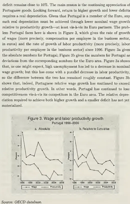
deficit remains close to 10%.

The main

reasonisthe continuing appreciation of

Portuguese goods.

Looking

forward, return to higher

growth

and

lower deficits

requires areal depreciation.

Given

that Portugalis a

member

ofthe Euro,

any

such real depreciation

must be

achieved through lower

nominal

wage

growth

relative to productivity

growth

—

at least vis-a-vis its

Euro

partners.

The

prob-lem

Portugal faces here is

shown

in Figure 3,

which

gives the rate of

growth

of

wages (more

precisely,

compensation

per

employee

in the business sector,

in euros)

and

the rate of

growth

oflabor productivity

(more

precisely, labor

productivity per

employee

in the business sector) since 1996. Figure 3a gives theabsolute

numbers

forPortugal; Figure 3bgivesthe

numbers

forPortugalas

deviations

from

the corresponding

numbers

for the

Euro

area. Figure

3a

shows

that, asone

might

expect, high

unemployment

has ledto a decreasein

nominal

wage

growth; but this has

come

with a paralleldecrease in labor productivity,

so the difference

between

the

two

has

remained

roughly constant. Figure

3b

shows

that, indeed, Portuguese relative

wage growth

has continued to exceed relative productivity growth. In other words, Portugal has continued to lose competitiveness vis-a-vis itscompetitors in the

Euro

area.

The

relative

depre-ciationrequired toachieve

both

higher

growth and

asmallerdeficit has notyet

materialized.

Figure 3.

Wage

and

labor productivity

growth

Portugal 1996-2006 a. Absolute_....

.

. .

b.RelativetoEuro area

Wage Productivity Wage Productivity

Should

Portuguese

macroeconomic

policyhave

been

different inthesecondhalf of the 1990s?

Given

what

we

now

know, namely

that expectations

were

too

optimistic, the answeris obviously yes.

The

relevantquestion is

however

what

should have

been

done

given

what was

known

then? Should

government

poli-cies

have

reduced the

boom,

limited the appreciation,

and

limited the current

account deficit?

The

question of

what

should have

been done

during the

boom

in Portugal is

now

academic.

But

the question is very relevant for Spain today. Since the

mid-1990s,steady

growth

hasledto alargedecreaseinthe

unemployment

rate,

down

from

20%

to

under

9%

today

—

a decreaseoften referred to asthe "Spanish

miracle." This

growth

has

been

sustained

by growth

inprivate spendingrather

than

public spending:

The

fiscal positionhas turned from a largedeficit in the

mid

1990s toasurplus of

1%

of

GDP

today.

At

the

same

time,

growth

has

come

with a steadyrealappreciation. Since 1995,

unit labor costs haveincreased

by

21%

relative to the

Euro

area.

The

current

accountdeficithasincreased

from rough

balanceinthe

mid

1990sto

9%

of

GDP

today. This raises aset ofobvious questions. Will Spain go through the

same

adjustment

processasPortugal?

Should government

policieshave beendifferent overthelastdecade?

Should

they havelimitedoutput growth,appreciation,

and

thecurrent account deficit?

What

should the Spanish

government

do today?

2

The

U.S. current

account

deficit

The

U.S. current accountdeficit has

dominated both

the

news and

much

ofthe

research ininternational

macroeconomics

inthe recentpast.3

My

purposehere

is onlyto pointto the aspects directlyrelevant to the

theme

ofthelecture, the

role of private saving

and

investment versus fiscal policy, the

way

the deficit

has

been

financed,

and

the rationality ofexpectations underlying decisions

and

investors's choices:

The

U.S. deficit is very large,

and

reflected in current account surpluses

vis-a-vis the

United

States in

most

regions of the world.

The

composition of the

3.

A

goodsurveyoftheoriesand factsis providedbyCline (2005).

An

insightfulanalysis of

the relative roles of saving, investment, andporfolio flows, intheUnited States andcreditor

corresponding current account surpluses for the third quarter of

2006

is given in Table 1.

Roughly

half is accounted

by

Asia, primarily

China and

Japan.

Roughly

one fourthis accounted for

by

Europe.

Of

the rest, an increasing but stiUsmall proportionisaccountedfor

by

the

Middle

East, reflectingthe increase

in oil prices.

Table

1.

The

U.S. current

account

deficit

and

its

counterparts.

2006-3, in billions

of

dollars, at

annual

rates.

Total 902

of

which

Europe

175 Asia 480

Canada

51

China

288

Latin

America

120

Japan

108

Middle

East 56

Source:

BE

A

International Transactions. Table 11,

January 2007

The

U.S. deficit

and

the corresponding foreign surpluses have

many

causes.

I believe that there is

now

a broad consensus

about

the following proximate

causes. First, low U.S. saving, reflecting primarily low private saving, but also

budget

deficits. Second, high foreign saving, particularly from Asia

—

what

Ben

Bernanke

(2005) has referred to as the "savingglut." Third, lowforeign invest-ment, in

both

Europe and

Asia. Fourth, a strong preference

by

investors for

U.S. overforeign assets. All four factors are

needed

to explain the

combination

ofcurrent accountbalances, thestrongdollar,low world realinterest rates,

and

apparently low expected returns

on

U.S. assets.4

The

important point for

my

purposes is that fiscal policies,

whether

in the

United

States or abroad, while notirrelevant,are clearlynotthe

main

cause ofthe U.S. current accountdeficit.

Private saving

and

investment decisions

—

sometimes mediated

through policy,

such as the combination of capital controls

on

capital outflows

and

reserve ac-cumulation in

China

—

around

theworld are.

Bank

lending,

which

was

central to the Latin

American

deficits, is nearly

ir-relevant in the case of theU.S. deficit.

The

composition offoreign holdings of

4. For more discussion, see in particular Bernanke (2005), Blanchard, Giavazzi, and Sa

(2005), and Caballero, Farhi,and Gourinchas (2006).

financialassets, for

both

stocks

and

flows,is giveninTable 2.

The

composition

of flows has

changed

over time, but the picture given

by

the stock

numbers

is

very clear: In the third quarter of 2006, gross foreign holdings of U.S. assets were roughly equal to 11 trillion dollars.

Of

those, roughly

40%

took the

form

ofholdingsofcorporateequities

and

directinvestment

—

a verydifferentpicture

from

the financing ofLatin

American

deficits.

Table

2.

Composition

of foreign

holdings

of

U.S.

assets (billions

of

dollars).

2006

Flows

Stocks Total 1,406 11,946 T-bills 101 2,069 Official holdings 111 1,371 Privateholdings -10 698 Corporate equities 112 2,601

Corporate bonds

377 2,596 Direct investment 185 2018

Source:

Flow

of Funds, FederalReserve Board. TablesF.107,

and

L.107. Stocks:

"Total U.S. financial assetsheld

by

therestofthe world", asof2006:3. Flows:

"Net acquisitionoffinancial assets

by

therestoftheworld", over thefirstthree

quartersof2006.

There

has

been

much

discussion as to

whether

investors behind these capital

flows

have

rational expectations.

There

is

no

question that, sooner or later,

current account deficits will have to decrease,

and

this will

most

likely require

asubstantialrealdepreciation of U.S. goods. For thisreason,

and

given thelow

U.S. interest rates, a

number

ofeconomists have argued that foreign investors

were

too optimistic

about

expected returns

on

U.S. assets. If investors have

a strong preference for U.S. assets however,

and

if they anticipate the rate

of depreciation to be positive

but

small, then the evidence against rational

expectationsis

much

weaker. Indeed, overthepastfewyears, financialinvestors

rather

than

these economists appear to have

been

right about the strength of

thedollar.

In short: Current "global imbalances" appear to

come

primarily

from

shifts

in private saving

and

investment. In the absence of strong evidence to the

contrary, the

assumption

that expectations are rational does not appear

un-reasonable. This takes us back to the question raised in this lecture.

Beyond

reducingthe U.S. budget deficit

—

a reduction

which

indeed appearsjustified

on

its

own,

but,

by most

estimates,

would

only

make

a dentinthe current account deficit

—

should the U.S. (andother)

governments

aim

atreducingtheremaining imbalances further?

Why,

and

ifso,

how?

3

A

benchmark

For this

and

the next three sections, I shall focus

on

the following

narrow

question:

Assume

current account deficits are the result ofprivate saving

and

investmentdecisions.

Assume

expectationsare rational. Shouldthe

government

intervene,

and

ifso

how?

To

do so, I startwith the following

benchmark:

The

model

The economy

goes

on

—

and

peoplelivefor

—

two

periods.Ineachperiod,people

derive utility

from

the

consumption

of

two

goods, tradables

and non

tradables,

and from

leisure.5

Utility is given by:

where

and

maxV =

U

+

/3U'

U

=

\og(C)

+

<j>\og(L)

\og(C)

= hog(C

T

)

+

^\og(C

N

)

where

primes denote second period variables,

Ct

and

Cn

denotethe

consump-tionoftradables

and

non-tradables respectively,

and

L

denotesleisure. (3 is the

discount factor.

As

is well

known,

the log-log assumptions,

and

the implication of equal

in-fratemporal

and

intertemporal elasticities of substitution eliminate a

number

5. Iintroducealabor-leisurechoicebecause,when,later, Iintroducedistortionswhichimply that employment ispotentially offthe labor supply, I wantto be ableto assess thewelfare

cost ofsuchadeviationandderivethe optimalpolicy.

of interesting issues, in particular with respect to the path of tradables

con-sumption.6; but they are fine for the points I

want

to

make

in this lecture.

Taking

tradables as thenumeraire,

and assuming

for simplicity that the world interest rate, theinterestrate intermsof tradables,isequaltozero, the

budget

constraint ofconsumer-workers isgiven by:

qC

N

+

C

T

+

q'C'

_N

+

C

_T

= A = w(N

t

+

N

N

)

+

w'(N

T

+

N'

N

)+ir

+

n'

with

N

T

+

N

N

= L-L,

N

T

+

N'

N

=

L

-

L'

where

A

is total wealth,

Nx

and

_Nn

denote

employment

in the tradables

and

non-tradables sector respectively, q

and

iu denote the relative price of

non-tradables

and

the

wage

in terms in tradables respectively. 7r is profit. For the

moment,

there is

no

government; I shall introduceit later.

On

the production side, competitive firms in the tradables

and

non-tradables

sectors

maximize

profitsubject to the following production functions:

Y

T

=

Nf,

Y

N

=

N

N

a

with similar equations holding for the second period. Capital is implicitly

as-sumed

tobe fixed, sothere is

no

investment decisionin themodel. I shallfocus

on

current account deficits

coming

fromvariations in saving.

The

equilibrium

Equilibrium requires that,ineach period, the non-tradables

and

the labor

mar-ket clear. This gives us four equations:

_

111.

,W

a/(a-l)

C

N

=

Y

N

=>

-

—

—

-

A =

—

2 1

+

p

q aq

18

1 w' /(0_1)

and

»r T r ,W,l/(a-l)

,W

,1/(0-1) ? 1

N

T

+

N

N

=

L-L

=>

(-)

+(—

)

=L

a aq 1

+

Q

w

6. Seeforexample ObstfeldandRogoff(1996), 4-4, equation(34), and Dornbusch (1983).

w' 1/(a_1) w' 1/(a_1)

6

where

1 '

' '

'W

A =

Y

T

+

Y^

+

qY

N

+

q'Y^

The

four equilibrium conditions are straightforward:

Wealth

is equal to the

presentdiscounted valueofoutputintermsof tradables.

Spending

on

tradables,

on

non-tradables,

and on

leisure are all proportional to wealth.

The

supply

of non-tradables

—

equivalently the

demand

for labor

from

the non-tradables

sector

—

is a decreasing function of the

wage

in terms of non-tradables; the

demand

for labor

from

the tradables sector is a decreasing function of thereal

wage

in terms oftradables.

If

=

1, (so thediscount rate is equalto theworld interest rate,

namely

zero), then the equilibrium is the

same

in

both

periods

and

the current account is

balanced. Itwill benotationally convenient to

assume

that, in thisequilibrium,

all quantities are equal to one, i.e. that Cj

=

Yi

=

TVj

=

L

=

C[

=

Y(

=

N[

=

L'

=

1, for i

=

T,N.

This in turn requires that

L

=

3

and

<j>

=

a/2. For

our purposes, these restrictions are innocuous.

Under

this normalization also, q

=

q'

=

1,

and

w

=

w'

=

a. It is alsoconvenient to introduce

w

=

w/a,

so in

the initial equilibrium

w =

w'

=

1.

Increased

impatience

and

current

account

deficits

I shall consider throughout the effects of

an

increase in impatience,

d0

<

0,

starting

from

=

1. Exactly the

same

analytical results

would

obtain

—

with a

minor

difference

which

Ishallpointout

below

—

if Ilookedinsteadatadecrease

inthe rate ofinterest at

which

thecountrycan borrow, dr

<

0,starting

from

r

=

—

an

experiment

which

would

capture for

example

part of

what happened

in Portugalinthe 1990s.

Other

shocks,for

example

the anticipation of increasesin productivityineithertheproduction oftradables or non-tradablesnextperiod,

would

lead todifferentanalyticalresults,butthe

same

generalconclusionsabout distortions,

and

the role for policy.

The

decrease in leads to

two

reallocations, intertemporal,

and

intratemporal:

•

Being

more

impatient, people

want

to

spend

more and work

lessin the

firstperiod.

•

Consumption

ofnon-tradables

and

tradablesincrease.

The

consumption

of tradables increases

more

than the

consumption

ofnon-tradables.

Tak-inga linear approximation

and

solvingthe equations

above

gives:

dC

_N

=

_\

_T

±

i

r

(-df3)

>

0;

dC

T

=

\{-dp)

>

16 —

la I

•

Employment

decreases(leisure increases).

Employment

innon-tradables

increases, but

employment

intradables decreases

by

more:

dN

_N

=

i^Mfl

>

0;

dN

T

=

j^i-dP)

<

•

The

price of non-tradables, q, increases.

So

does the tradables product

wage, w.

The

non-tradables product wage,

w/q

decreases:

dqv

=

-

l^±(-d0)

> dw

= ^—^(-dp)

>

2

3-2a

v '

3-2a

v '

The

real

consumption

wage,

w/y/q

increases.

• Increased

demand

for,

and

decreasedsupplyoftradables lead toacurrent

account deficit:

1 3

d (current account deficit)

=

-

-

—

—

{—dp)

>

£ o /id

• All changes hold with opposite signsin thesecond period.

•

As

a, the degree ofreturns to labor, increases, the production frontier

becomes

lessconcave,

and

it

becomes

easierto shiftproduction

between

tradables

and

non-tradables. Thus, the price of non-tradables

and

the

wage

increase

by

less.

The

productionofnon-tradablesincreases

by

more,

theproductionof tradables decreases

by

more,leading toalargercurrent

account deficit.

Thus, theequilibriumresponseexhibits

an

appreciation followed

by

a

deprecia-tion, and,correspondingly, adecreaseintheproductionoftradables followed

by

an

increaselateron.

The

current accountdeficit inthefirst period,

due

to both

higher

consumption

and

lower production of tradables, is offset

by

a current

account surplus in the second period.7

7. Underthealternativeassumption ofa decrease intheinterestrate,dr

<

0, allthe

equa-tionsabovewouldhold,with dr replacing d/3.Theonlydifferenceisthat,whilethe decrease

Clearly,

under

the assumptions

made

so far, the

outcome

is the first-best

out-come,

and

there is

no

need nor justification for

government

intervention.

The

questionsare then:

What may

be the relevant distortionsin this context?

How

do

they affect the equilibrium?

And

what

is the optimal policy? In the next

three sections, I explore three general directions:

The

potential role of

wage

or price rigidities in distorting the adjustment; the potential role of financial

constraintsindistortingadjustmentinthe tradables sector;the implications, if

any, ofthe possibility of

sudden

stops, in

which

the countryis either cut

from

world financial markets, or has to

pay

a

much

higher rate of return.

4

Wage

and

price

rigidities,

and

current

account

deficits

During

the 1990s, the increase in spending in Portugal

came

not only with

a current account deficit, but also an output

boom

and

a large increase in

employment.

This is in clear contrast to the

outcome

in our

benchmark,

where

the current account deficit

comes

with a decrease in

employment.

8

The

result in the

benchmark

is

more

general thanit

may

first appear:

The same

would be

true of an increase in expected productivity, leading to an increase

inwealth,

and

thus to an increase in both

consumption

and

leisure in the first

period.Thispoints tothe potentialroleof

wage and

pricerigiditiesindistorting

the adjustment:

The

price of non-tradables

and

the real

wage

may

not have

increased

enough

to achieve the desired infratemporal reallocation

between

the

two

sectors.

The

slump

since2000points toanother typeof potential

wage and

pricerigidity.

In the first best, shifting

from

a currentaccount deficit in the first period to a

current accountsurplusinthe secondrequires a decreasein therelativeprice of

non-tradables

and

intherealwage.

Such

arealdepreciationhas provendifficult to achieve inPortugal. This points to

something

like

downward wage

rigidity.

There

are

many

ways

of formalizing

wage and

pricedistortions, and, inthe end,

the details matter. In this section, I take a first pass

by

simply

assuming

that

both

q

and

w

do

not adjust at all,

and

thus

remain

equal to one throughout.

in Phas noeffectonwealth A, the decreaseinr increaseswealthbydA

=

-2dr.

8. Oneofthe

many

problemsinmappingany modeltothedata: Theinitialunemployment

rate in Portugal (7% in 1995) was probably higher than the naturalrate at thetime. Thus, someoftheemployment increasein the1990swasprobablyjustified.

I

assume

that

employment

is determined

by

labor

demand.

That

is, I

assume

that, inthe tradablessector,

demand

isdetermined

by

profitmaximization,

and

that, in the non-tradables sector, labor

demand

is determined

by

the

demand

for non-tradables.9 I leave the discussion of

downward wage

rigidity to later; it

turns outthatitseffectsarequitedifferent

from

thoseinthis section,

and

closely

related to the effectsoffinancial constraints, discussed inthenext section.

The

equilibrium

Inadditionto the assumptions that q

=

q'

=

1

and

w =

w'

=

1, theequilibrium is given

by

the condition that the non-tradables

market

clearseach period:

Y

N

= C

N

=>

Y

_N

!

2(1+/?)

Y'

_N

-C'

_N

=

Y'

_N

-^-j-^

where

2

+

Y

N

+

Y^

Output

of non-tradables is given

by

the

demand

for non-tradables,

which

is

proportional to wealth.

Wealth

is in turn equal to the

sum

of outputs in the

tradables

and

non-tradables sectors over the two periods.

Given

w =

w'

=

1,

profit

maximization

in the tradables sector implies constant production Y-j-

=

Y±

=

\.

Together, these

two

equations determine output of non-tradables in

both

pe-riods,

and

thus total output,

and

wealth.

Wealth

in turn determines the

con-sumption

of tradablesin

both

periods,

and by

implication the current account

balance.

Increased impatience

Consider again anincreaseinimpatience, adecreasein/?.

Given

wage and

price

9. Theusualrationalizationwouldbetoassumemonopolisticcompetitiveprice-settingfirms

in the non-tradablesector,willing to satisfy demandso longas price exceedsmarginal cost.

An

explicit formalizationwould then havean additional distortion, namely the presenceof

the monopolisticmarkup. Thisdistortion, so long as the markupisconstant,isirrelevant for

my

purposes.

rigidities, only one

mechanism

is

now

at work,

namely

intertemporal realloca-tion:

• People again

want

to

spend

more

and work

lessin the current period.

•

Consumption

ofnon-tradables

and

tradables increase,

and

now

increase

by

the

same

amount. Denote

first-bestchanges

by

a star.

Then:

dCN

=

\{-dj3)

>

dC

_N

>

0;

dC

T

=

\(-d(3)

=

dC*

_T

>

The

increase in the

consumption

oftradables is the

same

as in the first

best. But, because the price of non-tradables does not increase, the

in-crease in the

consumption

on

non-tradables is higher than in the first

best.

•

Employment

in non-tradables increases.

Employment

in tradables

re-mains

unchanged.So, incontrast tothefirstbest,

employment

increases:

dN

N

=

—

{-dp)

> dN*

_{N >}

0;

dN

T

=

> dN%

dN =

--!-

_(-dp)

_>

2a

• Increased

demand

fortradables,togetherwith

an

unchanged

supply, lead

to a current account deficit:

d (current account deficit)

=

-

{—d(3)

>

Because

the increase in

demand

for tradables is the

same

as in the first

best,

and

supply does not decrease

whereas

it does in thefirst best, the

current account deficit is actually smaller than in thefirst best.10

• All changes hold with opposite signs inthe second period.

Thus, the

economy

goes through a

boom

cum

current account deficit in the

first period, a

slump

cum

current account surplus in the second period.

Both

the

boom

and slump

areinefficient.

Workers

would

rather

work

less than they

do

inthe first period,

and

more

than they do inthe second period.

A

role for

policy?

10. Thisresultisnot robusttomoregeneralpreferences,and

may

notholdiftheintertemporal

and intratemporal elasticities of substitution are different. But the point that the current accountdeficitneednotbe largerundersuchrigidities, is general.

Can

policy

improve

the

outcome

and, ifso,

how?

A

full

answer

would

requirea

full other lecture. Let

me

briefly talk

about monetary and

tax policy,

and

then

deal

more

formallywith the potential role of

government

spending.

Depending on

theexact natureofrigidities,

monetary

policycangetthe

alloca-tion close to oreven

back

tofirst best.

Take

for

example

the case

where wages

are flexible

and

only

nominal

non-tradable prices are rigid

(w

isflexible

and

q

isfixedintermsofdomestic currency).

Then,

theappropriate

nominal

depreci-ation can achievethe first-best q,

and by

implication, replicate the

benchmark

allocation

—

eliminating

both

the

boom

and

theslump, while allowingfora

cur-rentaccountdeficit

and

intertemporalreallocation.In thepresenceof

both

wage

and

pricerigidities,

monetary

policycannot ingeneralsimultaneouslyreplicate

thefirst-bestvalues of q

and

w.

But

it canstill

improve

the outcome.11

For the countries within the

Euro

such as Portugal,

monetary

policy is not

available

however

—

at least with respect to country-specific shocks. This shifts

the focustowardsfiscalpolicy.

Here

again, giventhenatureofthe distortions,a

sufficientrichsetof taxes,say taxes

on

non-tradables

and on

labor, can achieve

first best. Let

me

however

focus

on

the potential role of

government

spending.

Let'sextend the

benchmark

toallow utilityto

depend on government

spending,

according to:

U

=

log(C)

+

cj>log(L)

+

a

log(G)

where

\ogG=

-\og{GT

l )

+

\\og{G

N

)

Assume

also that all

government

spendingis financedthrough

lump

sum

taxa-tion.

To

maintainthesimplepropertythat,if /?

=

1, allsteadystateproductions

are equal to one, <j>

must

now

satisfy <j>

—

(1

+

a)a/2; I

make

this

assumption

in

what

follows.

Given

the

symmetry

intreatment

between

private

consumption

and government

spending, it is clear that, in the absence of distortions, optimal fiscal policy

would

simplybe given by:

Gi

=

ad,

i

=

T,TV;

G

•

=

a

C[, _i

=

T,N

11. Thisiswelltraveled groundintheresearch onoptimalmonetarypolicyin an open

econ-omy. Seefor example Devereux and Engel(2006).

so, that for /3

=

1,

1+a

1+a

Ishallcallthis the "neutral"

component

offiscalpolicy,

and

focus

on

deviations

from

this neutral

component,

denoted dgi,i

= T,N

and

dg[,i

=T,N

for the

first

and

second periodrespectively.

Now

turn to the role of

government

spending in the case of price

and wage

rigidities.

Given

the

symmetry

offirst-period

and

second-period effects ofthe

decrease in /?, it follows that the optimal policy satisfies dg'

_N

=

—dg^

and

dg'r

=

—dgr-

Thus,

we

can focus

on

the determination of just

dg^

and

dgr-Going through

the characterization of the equilibrium,

now

in the presence of the government, gives:

dY

N

=

\{-dP)

+

dg

_N

,

dCN

=

i—

L-(-d/3),

dGN

=

I-5L_(-d/3)

+

dg

N

z

zi

+

q

z l

+

a

An

increasein

government

spending

on

non-tradablesincreases output of

non-tradables one-for-one. It has

no

effect

on

the

consumption

of non-tradables.

The

reason

why

consumption

is unaffected is the absence ofa wealth effect:

Any

increase in

dg^

is expected to be offset

by an

equal decrease in dg'

_N

;

any

increasein

dY^

induced

by

higher

dg^

is alsoexpected to

be

offset

by an

equal

decrease in

dY^:

dY

T

=

0,

dC

T

=

\

-L-

{-dp),

dG

T

=

_I

-~

(-dp)

+

dg

_T

z 1

+

a

Z 1

+

a

An

increase in

government

spending

on

tradables has

an

effect neither

on

pro-duction nor

on consumption

of tradables. Thus, it affects the current account deficit one-for-one.

The

reason

why

consumption

is unaffected is again the

ab-senceofa wealtheffect.

Any

increasein

dgx

isexpectedto

be

offset

by an

equal decrease in

dg

_T

.

12

Thus, the right tool to reduce the inefficiency is clearly dg^.

A

negative

dg^

in the first period, associated with apositive dg'

_N

inthe second period allows

the

government

toeliminatethe

boom

and

the slump.

A

negative dgx, followed

by

a positive dg'

_T

would

reduce the current account, but have no effect

on

the

inefficiency. This suggests that theoptimal policyis to use only

dg^

and

dg'

_N

.

12. Theextreme formofsomeoftheseresultsdependsagainonthelog-log restrictions. But

themessage abouttherelativeeffectsofdgN and dgr isgeneral.

Indeed, under a quadratic approximation to the utility function

and

a linear approximation to the equilibrium conditions, the optimalpolicyis given by:

2(a

+

a

+

aa)

This policy leaves the current accountdeficit unaffected, but reducesthe

boom

and

theslump.

The

message

from

thisfirst extensionis that price

and

wage

rigidities

may

well

distort the allocation.

The

optimal policy

may

not

however

be

to reduce the

current account deficit. Indeed, inthe simplecase

worked

out here, the current

account deficit is unaffected.

One

question is

whether

more

asymmetric

forms

ofrigidity, such as

downward

wage

rigidity,

would

leadto differentconclusions.

The

answer

is yes,

and

Ishall return to this below.

5

Financial

constraints,

and

current

account

deficits

Adjustment

inthe first best implies first a decrease, thenan increase (equal to

twice theinitialdecrease) intradables output.

One

worry

isthat it

may

indeed

be difficultforthetradables sector to

expand

aftera long periodof appreciation

and

low production.

One

may

think of a

number

of reasons

why

this

might

be. Internal costs of

adjustment are not the issue:

These

will indeed affect the adjustment,

and

thus affect in turn first-period decisions

and

the current account deficit; but,

absent other considerations, the

outcome

will still

be

the first-best outcome,

and

there is

no

role for

government

policy.

Other

distortions

may

however be

relevant.

Krugman

(1987)

emphasized

for

example

external learning

by

doing,

and

the fact that a long period of low production

may

lead to

permanently

lower productivity. Others have

emphasized

financial constraints, the fact that

the tradables sector

may

not, after a long period oflowprofits, have thefunds

needed

to invest

and

increase production later on.

I explore this idea

by

making

a simple, ifhighly reduced form, assumption. I

assume

that production oftradables in the second period is givenby:

w

a~1

Y±

=

min(

Y

_T

,

(-)

)

Production

of tradablesisequal tothe

minimum

oftheprofit

maximizing

level

of

output

in the second period,

and

the level of production oftradables in the

firstperiod. Fortheshock

we

shalllookat,

namely

anincreaseinimpatience,the

constraint is binding,

and

second-period tradables output is thus constrained

to be

no

larger than first-period output.

Some

generality

would

be obtained

by

allowing the parameter in front offirst

periodoutput tobe different

from

one; but thisisinessential.

A

rough

justifica-tion for this

assumption

may

be the following: Tradables firms can

borrow

up

to

some

multiple offirstperiod earnings

—

which

areproportional tooutput

—

to

pay

the second-period

wage

bill,

which

is itself proportional to second-period output.

A

more

explicit

and

richer micro-grounding is given

by

Caballero

and

Lorenzoni (2006):

During

the appreciation period, firms incur losses.

Because

of financial constraints, these losses

may

force

them

to decrease their capital

stock

beyond

what

would

be efficient, putting constraints on the recovery in

the second period.

Another

issueis

whether

firmsinthe tradables sector internalizethis constraint

when

taking

output

decisions in the first period (and so choose a higher level

ofproduction in the first period inorder to relaxthe constraint

on

production in the second period). This

depends on whether

the constraint holds at the

level of the firm or for the tradables sector as a whole. I

assume

that the

constraintholdsforthe sector asa

whole

(thatthereis,forexample, a

segmented

financial

market where

only tradables firms can participate),

and

so firms

do

not internalize it intaking decisionsinthe firstperiod.

The

equilibrium

Equilibrium requiresthat the tradables

market

and

the labor

market

eachclear

ineach period, yielding four equilibrium conditions. Let

me

introduce the

gov-ernment from

the start, soas to prepare forthe discussion of policy later on:

C

N

+

G

N

=

Y

N

=>

1-LpkA

+

dgn

=

(f) o/( ° !)

N

T

+

N'

N

=

L-L'

=> ffii/(*-D

₊

(f)^"-1)

=

I-^A

where

A =

(YT

+

Y

_T

+

q

Y

N

+

q' _Yj,)

-

_(q dg

_N

+

q' _dg'

N

+

dg

_T

+

dg'

_T

)

Leaving aside the additional terms

coming from

the presence of fiscal policy,

the onlydifference

between

these equations

and

thoseofthe

benchmark

arein

the specification ofthe second-period

demand

for labor in the tradables sector

in the fourth equation:

Assuming

the constraint is binding, labor

demand

in

the second periodis equal to labor

demand

in the first period,

and

so

depends

on

the first-period rather than the second-period realwage.

The way

fiscalpolicy entersisalsostraightforward,

_dgn

and

dg'

_N

directlyaffect the

demand

fornon-tradables,

both

directly

and

throughtheir effect on wealth.

dgT and

dg'

_T

affectspending

and

laborsupply onlyto theextentthat theyaffect

wealth. This is

what

is

shown

in thelast equation.

Increased

impatience

Consider

now

the effects of an increase in impatience, d(5

<

0,

assuming

first

that there is

no

fiscal policy response, so all dg's are equal to zero.

Then:

• Just as in the

benchmark,

people

want

to intertemporally substitute,

enjoy

more

consumption

and

more

leisure in the first period.

But

they

now

also take into account that lower tradables production in the first

periodimplieslower tradablesproductioninthesecond period,

and

thus lower

income

in the second period. This leads to a decrease in their

wealth,

and

thus lower

consumption and

higher labor supply in

both

periods.

• Thus,the

demand

fortradables

and

non-tradablesincreases, but,in

both

cases,

by

less

than

in the firstbest:

dC

_N

+dG

N

= dY

N

=

J(-d/3)

>

dC'

_N

+dG'

_N

=

dY^

=

%{-d0)

>

D

dC

T

+

dG

T

=

^—^-(-dp)

>

dC'T

+

dG'T

=

-i±i£(-d/?) <

6

Both

because the increasein non-tradables outputin the first period is

smaller than in the first best,

and

because the decrease in labor supply

is smaller than in the first best, the decrease in tradables output in the

first period is alsosmaller than in the first best.

As

the financial

market

constraint is binding, the decrease in tradables output in the second

period is the

same

as in thefirst period.

dy

r

=

-|(-d/3)<o

dy^

=

-^(-d/?)

<

o

Higher

demand

and

lower supplyof tradables lead to acurrent account

deficit.

The

current account deficit is

however

smaller

than

in the first

best:

d(current account deficit

=

-(—

d(3)

>

Because

the increase in the

demand

for non-tradablesis smallerthan in

the first best, so are theinitial appreciation

and wage

increase:

dg

=

^(-d/3)>0

dq'

=

_l±£(-d/3) <

dw

=

^-—

-(-dp)

>

dw'

=

-

a

^{-dp)

<0

In contrast to the first distortion, adjustmentsin the second period are

not mirror images ofthose in the first period.

Output

oftradablesgoes

down

in

both

periods, output of non-tradables goes up.

The

current

account deficit

comes

with a

slump

in the tradablessector.

The

misallocation of labor

between

the

two

sectorsinthe second period

leads to a decrease inwealth,

and

to afirst-order loss in welfare:

dA

=

-|(-d/3)

<

0;

dV

=

-a{1

+

a

_\

-d/3)

<

Optimal

fiscal

policy

Given

this

outcome,

is there a role for fiscal policy? Intuition suggests that

there is:

A

decrease in

Gn

can decrease the

demand

and

the production of

non-tradables,

and

thus increase the production of tradables in the first

pe-riod and,

by

implication, in the second period. Increases in either

Gt

or G'

_T

,

while theyhave

no

directeffect

on

the productionof tradables, decrease wealth

and

thusprivate spending, includingspendingon non-tradables. This again

in-creases production of tradables in the first period,

and by

implication, in the

second period. This suggeststhat optimalpolicyincludes decreasesinG/v,

and

increases in

Gt

and

G'

_T

.

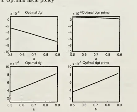
Figure

4.

Optimal

fiscal

policy

X 10~3 Optimaldgn x-jo -3_{Optimaldgnprime} x10 0.7 a Optimaldgt 0.9 0.7 a x -|q-3_{Optimaldgtprime} 0.9

This is indeed the case. Figure 4 gives the optimal values of the dgi's (the

deviation from neutral fiscal policy) obtained

by

maximization of a

second-order

approximation

to the utility function subject to a linear approximation

ofthe equilibrium conditions given above.

The

figure gives values for

a

=

0.5

and

a ranging

from

0.5 to 0.9. It

shows

that, indeed, optimal

dg^

is negative,

optimal dg'

_N

is close to zero,

and

optimal

dgr and

dg'

_T

are equal to each other

and

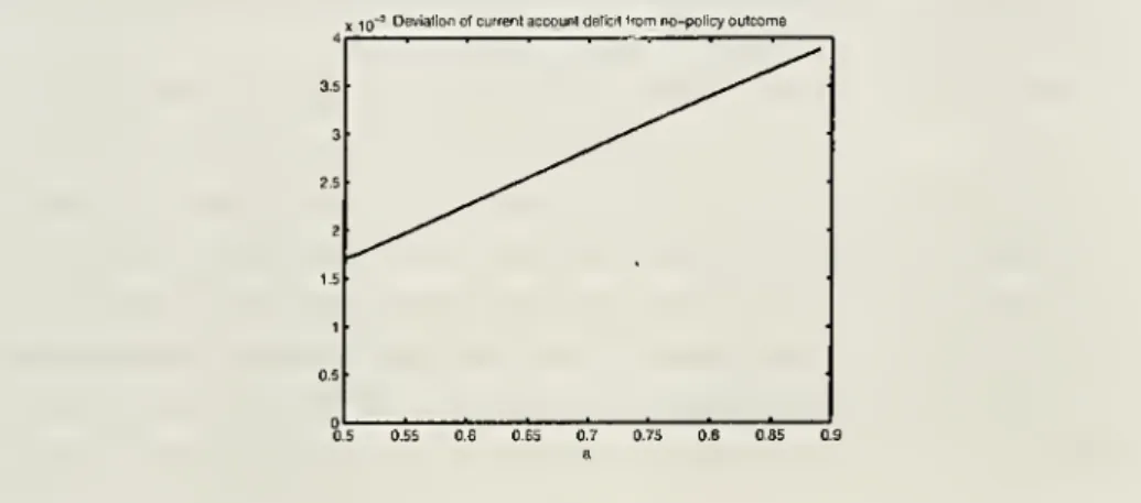
positive.

Figure5

shows

the deviation of the currentaccount deficit

from

itsvalueabsent

fiscalpolicy.

Note

thatthe current accountdeficitis actually larger under

opti-mal

fiscalpolicy (forexample, 0.004 higherifa

=

0.9).

The

reason isthatwhile

thedecrease in

government

spending

on

nontradables increases the production

of tradables, the optimal policyalso requires

an

increasein

government

spend-ing

on

tradables,

which

directly increases the currentaccount deficit. Isee this

result not as a

major

implication, but, again, as a

warning

that the presenceof

distortions does not necessarily require policies

aimed

at reducingthe current

account deficit.

Figure

5.

Current account

deficit,

with

and

without

fiscal

policy

Deviationofcurrentaccountdeficit'rom no-policyoutcome

0.55 0.6 0.65 0.7 0.75 0.6 0.85 0.9

The

message

from this second extension is that, to the extent that financial

constraints matter in the tradables sector, there is indeed a role for policy to

limit reallocation in the first period.

The

optimal policy

however

may

or

may

not decrease the current account deficit.

How

important are the relevant financial

market

imperfections,

and

how

much

do

theylimitreallocation?13

One

might

guessthat tradables firmsinrich coun-tries

would

be

among

those with the best access tofinancialmarkets,

and

thus

would be

least likely to be financially constrained. But, as far as I can tell,

we

do

not

know. Recent work by

Calvo, Izquerdio,

and

Talvi (2006) suggests

that,eveninArgentinaafterthe collapse

and

thedisorganization ofcredit

mar-13. The question has been explored, in a different but related context, by Caballero and

Hammour

(2005), who have looked at whether recessions lead tothe disappearance oflow productivity versusfinanciallyconstrainedfirms.

kets, tradables firms have

been

able to increase production in response to the

(admittedlyverylarge) peso depreciation.

Let

me

return briefly to an issue I left aside in the previous section,

namely

the implications of

downward wage

rigidity.

Under

the

assumption

that the

wage

in terms of tradables can increase but cannot decrease, the equilibrium

looks very

much

like the equilibrium I havejust characterized. In response to

an

increaseinimpatience,

downward

rigidityprevents thefirst-bestreallocation

ofproduction:

The

real

wage

goes

up

in the first period, but cannot go

down

in the second period, leading to lower production of

both

tradables

and

non-tradables in the secondperiod. Anticipations oflower future income,

and

thus

lower wealth (relative to first best), lead people to

want

to

consume

less

and

work

more

inthe first period (again,relative to first best).

The

result is a lower

current accountdeficit

and

boom

in the firstperiod,

and

an output

slump

cum

current account surplus inthe second period.

Note

that,

under

financial

market

constraints,the labor

market

clears inthe

sec-ond

period, but the allocationis distorted towards non-tradables; under

down-ward

rigidity, the labor

market

does not clear,

and both

the production of

tradables

and

non-tradables are lower. In terms of policy however, the

con-clusions are roughlysimilar.

Optimal

policy requires measures

which

limit the

wage

increaseinthefirstperiod, either

by

decreasing

demand

for non-tradables

or the supply of labor.

6

Sudden

stops, distortions,

and

policy

I suspect that,

up

to this point, I have not dealt with the

main

worry

in the

mind

ofa

number

ofeconomists

and

policymakers,

namely

"suddenstops."This

is the

worry

that a country

may

find itselfsuddenly cut

from

world financial markets, or

more

realistically for a country such as the United States, that

foreign investors

may

ask suddenlyfor a

much

higher rate of return.14

That

sudden

stopscan

happen

is

amply

demonstrated

by history,

most

recently

by

theAsiancrisis.15

That

they canlead tosharpdepreciations,

and sometimes

14. Thisis forexamplea recurringtheme inNourielRoubini'sblogcommentary on the U.S.

current accountdeficit.

15. TheAsiancrisisindeedshowsthatsuddenstopscanhappeneveninthe absenceof large

current accountdeficits.