Transport on Riemannian Manifold for Connectivity-based Brain Decoding

HAL Id: hal-01185200

https://hal.inria.fr/hal-01185200

Submitted on 19 Aug 2015

HAL is a multi-disciplinary open access

archive for the deposit and dissemination of

sci-entific research documents, whether they are

pub-lished or not. The documents may come from

teaching and research institutions in France or

abroad, or from public or private research centers.

L’archive ouverte pluridisciplinaire HAL, est

destinée au dépôt et à la diffusion de documents

scientifiques de niveau recherche, publiés ou non,

émanant des établissements d’enseignement et de

recherche français ou étrangers, des laboratoires

publics ou privés.

Transport on Riemannian Manifold for

Connectivity-based Brain Decoding

Bernard Ng, Gaël Varoquaux, Jean-Baptiste Poline, Michael D Greicius,

Bertrand Thirion

To cite this version:

Bernard Ng, Gaël Varoquaux, Jean-Baptiste Poline, Michael D Greicius, Bertrand Thirion.

Transport on Riemannian Manifold for Connectivity-based Brain Decoding.

IEEE Transactions

on Medical Imaging, Institute of Electrical and Electronics Engineers, 2015, PP (99), pp.9.

�10.1109/TMI.2015.2463723�. �hal-01185200�

Abstract—There is a recent interest in using functional

magnetic resonance imaging (fMRI) for decoding more naturalistic, cognitive states, in which subjects perform various tasks in a continuous, self-directed manner. In this setting, the set of brain volumes over the entire task duration is usually taken as a single sample with connectivity estimates, such as Pearson’s correlation, employed as features. Since covariance matrices live on the positive semidefinite cone, their elements are inherently inter-related. The assumption of uncorrelated features implicit in most classifier learning algorithms is thus violated. Coupled with the usual small sample sizes, the generalizability of the learned classifiers is limited, and the identification of significant brain connections from the classifier weights is nontrivial. In this paper, we present a Riemannian approach for connectivity-based brain decoding. The core idea is to project the covariance estimates onto a common tangent space to reduce the statistical dependencies between their elements. For this, we propose a matrix whitening transport, and compare it against parallel transport implemented via the Schild’s ladder algorithm. To validate our classification approach, we apply it to fMRI data acquired from twenty four subjects during four continuous, self-driven tasks. We show that our approach provides significantly higher classification accuracy than directly using Pearson’s correlation and its regularized variants as features. To facilitate result interpretation, we further propose a non-parametric scheme that combines bootstrapping and permutation testing for identifying significantly discriminative brain connections from the classifier weights. Using this scheme, a number of neuro-anatomically meaningful connections are detected, whereas no significant connections are found with pure permutation testing.

Index Terms—brain decoding, connectivity, fMRI,

Riemannian geometry, transport on manifolds

Manuscript received July 29, 2015. This work was supported in part by the Natural Sciences and Engineering Research Council of Canada. Asterisk indicates corresponding author.

*Bernard Ng is with the Functional Imaging for Neuropsychiatric Disorders Lab, Stanford University, Palo Alto, CA, USA, 94305 (email: bernardyng@gmail.com).

Gael Varoquaux is with the Parietal team, INRIA Saclay, Gif-Sur-Yvette, France, 91191 (email: gael.varoquaux@normalesup.org)

Jean Baptiste Poline is with the Parietal team, INRIA Saclay, Gif-Sur-Yvette, France, 91191 (e-mail: jbpoline@gmail.com)

Michael Greicius is with the Functional Imaging for Neuropsychiatric Disorders Lab, Stanford University, Palo Alto, CA, USA, 94305 (email: greicius@stanford.edu)

Bertrand Thirion is with the Parietal team, INRIA Saclay, Gif-Sur-Yvette, France, 91191 (email: bertrand.thirion@inria.fr)

Copyright (c) 2015 IEEE. Personal use of this material is permitted. However, permission to use this material for any other purposes must be obtained from the IEEE by sending a request to pubs-permissions@ieee.org.

I. INTRODUCTION

ecently, there has been a growing interest in using functional magnetic resonance imaging (fMRI) for brain decoding applications [1, 2]. Most studies have focused on decoding brain volumes acquired during brief, externally-guided tasks, in which the task timing is strictly controlled by the investigators through presentation of stimuli. Under this typical setting, each brain volume of a particular discrete time instance is classified into one of multiple cognitive states based on the blood oxygenation dependent level (BOLD) signal intensity of the voxels taken as features. However, during daily activities, the brain spends most of its time processing in a continuous, internally-guided fashion [3]. This more naturalistic, self-driven aspect of the brain is not well captured by the typical block design and event-related paradigms [4]. A handful of recent studies have explored the feasibility of decoding internally-driven states [4-6], in which subjects perform tasks, such as recalling events of their day, continuously over several minutes in an unconstrained manner. The widely-studied resting state also falls in this category of self-guided brain state, although not usually described under such light. In particular, a number of longitudinal studies have explored how interventions, e.g. motor [7] and memory training [8], between acquisitions alter resting state activity. The classification task under this setting involves separating resting state connectivity patterns before and after interventions [8]. Under these experimental frameworks where each time instance is no longer associated with a clear class label, the set of brain volumes over the entire task duration is usually taken as a single sample and estimates of functional connectivity between brain regions, e.g. Pearson’s correlation between brain region time courses, are typically used as features [4, 5]. Employing connectivity as features falls in line with the current understanding that most brain functions are mediated via the interactions between brain regions.

Directly using Pearson’s correlation (i.e. normalized covariance) as features for classifier learning has a fundamental limitation. Since covariance matrices, Σ, live on the space of positive semidefinite cone, i.e. vTΣv ≥ 0 for all vectors v [9, 10], elements of Σ are inter-related, which violates the uncorrelated feature assumption implicit in most classifier learning algorithms. In particular, many

Transport on Riemannian Manifold for

Connectivity-based Brain Decoding

Bernard Ng, Gael Varoquaux, Jean Baptiste Poline, Michael Greicius, and Bertrand Thirion

classifier learning algorithms are unstable in the face of correlated features, i.e. small perturbations on the training data can alter the relative weighting of the features [11]. Worsening the situation is the lack of training samples. Connectivity-based classifier learning is usually performed on data from multiple subjects to keep scan time reasonable for each subject, i.e. reliable covariance estimation requires at least several minutes of fMRI data per condition. For typical studies, the number of subjects is no more than thirty or so [12]. Hence, the sample size is rather small. As a result, the estimated classifier weights would have high variance. Combined with the effect of correlated features, the generalizability of the classifiers is limited, and identification of significantly discriminative brain connections from the classifier weights is nontrivial.

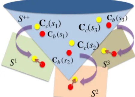
In this paper, we target two complementary problems associated with brain decoding. Our primary goal is to develop a classification approach that is more suited for taking covariance matrices as features. Our secondary goal is to devise a statistical inference scheme for identifying significant features from the learned classifier weights. Both problems hinge on how correlated the features are, which we deal with using tools from Riemannian geometry. Specifically, Riemannian geometry generalizes the notion of tangent vectors in Euclidean space to manifolds [10]. This facilitates computation of geodesic distance, which in turn enables statistics on manifolds, such as the positive definite cone [10]. The heart of our correlation reduction approach is to treat the positive definite cone as a Riemannian manifold and use the associated manifold operations to project the estimated covariance matrices of all subjects onto a common tangent space of this manifold. On the tangent space, elements of the covariance matrices are no longer linked by the positive semidefinite constraint [9]. Thus, the impact of correlated features on classifier learning is alleviated. Projection requires selecting a base point in the manifold that is close to the covariance matrices to be projected. Due to inter-subject variability in brain connectivity patterns, there is unlikely a single base covariance matrix that is close to the covariance matrices of all subjects. If we find a subject-specific base covariance matrix for each subject and perform projection, the projected covariance matrices will lie in different tangent spaces across subjects, hence not comparable, as illustrated in Fig. 1.

To bring the covariance estimates of different brain states of all subjects to a common tangent space, we propose a matrix whitening transport1

1

A preliminary conference version of this work appeared in [8].

. The underlying idea is to find a subject-specific base covariance estimate that is close to all state covariance estimates of each subject and use it for matrix whitening. The resulting state covariance estimates of all subjects would be close to the identity matrix. Thus, we can use the tangent space at the identity matrix as the common space for projection. In effect, we are removing the commonalities between cognitive states

for each subject in a nonlinear fashion, and using the residual for classifier learning.

Fig. 1. Problem of inter-subject variability on Riemannian projection. Projection requires the covariance matrices to be close to a base point at which projection is performed. Due to inter-subject variability in brain connectivity patterns, no single base covariance matrix would be close to the state covariance matrices of all subjects, Cc(s), s = s1, s2, s3. Using

subject-specific base covariance matrix, Cb(s), for projection would lead

to the resulting projected state covariance matrices to lie in different tangent spaces (S1_{, S}2_{, S}3_{), hence not comparable.}

The entailed manifold operations require the covariance estimates to be positive definite, which we achieve using a couple of regularization techniques, namely oracle approximating shrinkage (OAS) [13] and sparse Gaussian graphical model (SGGM) [14]. To estimate base covariance matrices, we examine several mean covariance estimation methods, including Euclidean mean of the state covariance estimates of each subject, Log Euclidean mean [15], and covariance computed on concatenated brain region time courses over cognitive states. For comparison with our proposed transport, we explore the concept of parallel transport, which provides the least deforming way of moving geometric objects along a curve between two points on a manifold [16, 17]. To perform parallel transport, we use the Schild’s ladder algorithm [18, 19], which dates back to the 70’s and has recently been revitalized for applications, such as longitudinal deformation analysis [20] and object tracking [17]. As validation, we apply our approach to fMRI data collected from twenty four subjects undergoing four experimental conditions, and compare it against directly using Pearson’s correlation and its regularized variants as features. We show that reducing the dependencies between the connectivity features using our approach significantly increases classification accuracy.

Further, to facilitate result interpretation, we propose a scheme that combines bootstrapping and permutation testing for identifying significant brain connections from classifier weights. This problem falls under the area of high dimensional inference where multiple features are jointly considered, and it is the distinct effect of a feature that is tested, with other features semi-partialed out to infer significance. This open problem is receiving growing attention from the statistics community with a focus on regression [21, 22]. Our proposed scheme addresses this problem for the classification setting. Detection of neuroanatomically relevant brain connections is shown.

) (s1 b C Cc(s1) S++ S1 Cb(s2) Cc(s2) S2 ) (s₃ b C Cc(s3) S3

II. METHODS

Treating the positive definite cone as a Riemannian manifold and using the associated operations (Section II-A), we propose a matrix whitening transport for covariance projection (Section II-B), and compare it against parallel transport with Schild’s ladder (Section II-C). To ensure that the state and base covariance estimates are positive definite, we employ OAS and SGGM (Section II-D) and compare various mean covariance estimation methods (Section II-E). Support vector machine (SVM) [23] is used for classification (Section II-F) and a non-parametric scheme is devised for identifying significantly discriminative brain connections (Section II-G).

A. Manifold Operations for Positive Definite Matrices

Let A be a d×d positive definite matrix. Since A ϵ S++, where S++ denotes the positive definite cone, elements of A are inter-related under the constraint: vTAv > 0 for all vectors v.

One way to remove this constraint is to consider S++ as a Riemannian manifold and project A onto the tangent space at a d×d base point, B ϵ S++, using the Log map [10]:

2 / 1 2 / 1 2 / 1 2 / 1 ) ( ) (A B B AB B B = logm − − Log , (1)

where logm(∙) denotes matrix logarithm and LogB(A) is the tangent vector at B “pointing towards” A with B assumed to be close to A [17]. Since elements of LogB(A) are not linked by the positive definite constraint [10], in the context of connectivity-based brain decoding with A being a positive definite covariance estimate, using elements of LogB(A) as features alleviates the impact of correlated features on classifier learning. More generally, a major difficulty with working in S++ is that the resultant from even standard operations, such as subtraction, may not reside in S++, since

S++ is not a vector space. An elegant solution to this problem is to operate in the tangent space and project the resultant back onto S++ using the inverse mapping, i.e. the Exp map (2), which guarantees positive definiteness [10].

2 / 1 2 / 1 2 / 1 2 / 1 ) ( ) (A B B AB B B = expm − − Exp , (2)

where expm(∙) denotes matrix exponential. By combining (1) and (2), one can compute the geodesic, i.e. local shortest path on S++, between two positive definite matrices as follows [10]:

] 1 , 0 [ )), ( ( ) (t =Exp t⋅Log A t∈ γ B B . (3)

This concept of geodesic will be important for parallel transport, as discussed in Section II-C.

B. Proposed Matrix Whitening Transport

Let Cc(s) ϵ S++ be the d×d state covariance matrix of

subject s associated with experimental condition c, where d is the number of brain regions. Also, let Cb(s) ϵ S++ be a d×d

base covariance matrix of each subject s that is close to Cc(s)

for all c. If we simply apply (1) to project Cc(s) onto the

tangent space at Cb(s), all subjects’ projected covariance

matrices will lie in different tangent spaces (i.e. Cb(s) are

different across subjects due to inter-subject variability), hence not comparable with each other (Fig. 1). Instead, under the assumption that Cb(s) is close to all Cc(s) of subject s, we can

use Cb(s) to approximately whiten Cc(s) for each subject, so

that the resulting covariance matrices, Cb(s)-1/2Cc(s)Cb(s)-1/2,

would be close to the identity matrix, Id×d, for all subjects.

Thus, the tangent space at Id×d can serve as the common space

across subjects for projection, which reduces to taking the matrix logarithm of the whitened state covariance matrices:

) ) ( ) ( ) ( ( ) (s =logm s −1/2 s s −1/2 dC_c C_b C_c C_b , (4)

since Log_I (A) I1_d/2_dlogm(I_d1/_d2AI_d1/_d2)I1_d/2_d logm(A)

d d = × = − × − × × × .

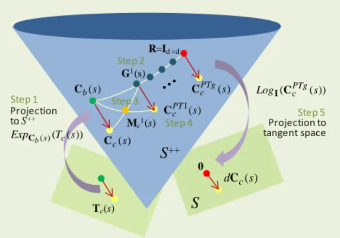
The proposed whitening transport is summarized in Fig. 2.

Fig. 2. Proposed matrix whitening transport. By whitening the state covariance matrix, Cc(s), with a base covariance matrix, Cb(s) that is close to

Cc(s) for all c, the resulting state covariance matrix would be close to the

identity matrix, Id×d, which enables projection to be performed at a common

tangent space for all subjects. Elements of the projected state covariance matrix, dCc(s), are not linked by the positive definite constraint, which

alleviates the problem of correlated features in classifier learning.

In effect, we are isolating the distinctive attributes of the different brain states by removing their commonalities in a nonlinear fashion, and using the residual for classification. We note that (4) is analogous to the manifold operation that we deployed in [9] for building an one-class classifier to discriminate subject types, but we are proposing here a new perspective on the entailed matrix multiplication as a transport to the neighborhood of Id×d, which justifies why projection

onto the tangent space at Id×d is legitimate. To generate Cb(s)

that produces a whitening effect, we use the mean Cc(s) over c

for reasons discussed in Section II-E. Also worth noting is that with Cb(s)-1/2Cc(s)Cb(s)-1/2 viewed as a matrix whitening

operation as proposed here, (1) can be interpreted as: whitening A with B to bring A close to Id×d, projecting the

whitened A onto the tangent space at Id×d, and dewhitening the

projected, whitened A to translate it back to the base point B. To demonstrate the necessity of matrix whitening before projection, we compare (4) with the case of setting dCc(s) to

logm(Cc(s)), i.e. no transport before projection, which is

exactly the Log-Euclidean approach widely employed by the diffusion MRI community for extending Euclidean operations to tensors [15]. Also, to test the need for employing manifold operations, we examine another simplification to (4), which we refer to as the Euclidean approximation. Specifically, we remove the commonalities between the Cc(s)’s of each subject

in a linear fashion and apply a first order approximation to the matrix logarithm, i.e. logm(A) ≈ A – Id×d, resulting in dCc(s) =

Cc(s) ‒ Cb(s) for the off-diagonal elements. Since linear

subtraction can result in non-positive definite matrices, the first order logm approximation is necessary. Also, for connectivity-based decoding, only the off-diagonal elements

) (s c C _{1/2 1/2} ) ( ) ( ) (s − _c s _b s − b C C C ) ) ( ) ( ) ( ( s −1/2 s s −1/2 logmC_b C_c C_b ) (s dC_c

S

S

corresponding to between-region connectivity are of interest.

C. Parallel Transport with Schild’s Ladder

Another way of transporting the state covariance matrices of all subjects to a common tangent space is to use parallel transport [16], which provides the least deforming way of moving geometric objects along a curve on a manifold [17]. One way of performing parallel transport is to use the Schild’s ladder algorithm [18, 19], as summarized in Fig. 3.

Fig. 3. Schild’s ladder. Let Tc(s) be the tangent vector corresponding to

the Log map of Cc(s) at Cb(s). Parallel transport of Tc(s) to the tangent

space at R involves the following steps. Step1: Project Tc(s) onto S++,

which is just Cc(s). Step2: Generate a discretized geodesic, Gi(s), from

Cb(s) to R. Step3: Compute the midpoint, Mc1(s), of the geodesic

connecting Cc(s) and G1(s). Step4: Find the one-step transported state

covariance matrix, CcPT1(s), which is twice the geodesic distance from

Cb(s) to Mc1(s). Step5: Repeat until R is reached, and apply Log map to

find the parallel transported covariance matrix, dCc(s).

Let Tc(s) = LogCb(s)(Cc(s)) be a d×d projected covariance

matrix, i.e. a tangent vector, at Cb(s). Parallel transport of

Tc(s) from the tangent space at Cb(s) to the tangent space at R

ϵ S++ _{using Schild’s ladder involves the following steps. Step1:}

Determine using (3) the point on S++ that is unit distance from

Cb(s) along the geodesic uniquely defined by Tc(s) [10], which

is exactly Cc(s) since Cc(s) = ExpCb(s)(1∙LogCb(s)(Cc(s))). Step2:

Generate a discretized geodesic from Cb(s) to R: Gi(s), i = {1,

…, g}, where g is the number of points along the geodesic.

Step3: Find the midpoint of the geodesic joining G1(s) and

Cc(s): Mc1(s) = ExpCc(s)(0.5∙LogCc(s)(G1(s))). Step4: Construct a geodesic from Cb(s) to Mc1(s) and move twice the distance to

find the one-step parallel transported state covariance matrix:

CcPT1(s) = ExpCb(s)(2∙LogCb(s)(Mc1(s))). Step5: Repeat this

procedure for all Gi(s), i = {1, …, g} until R is reached, and apply (1) to find the parallel transported Tc(s): dCc(s) =

LogR(CcPTg(s)). Note that we assume doubling t in (3) results

in double the geodesic distance, which we empirically verified on real data (Section III) using the affine invariant metric in [10] to estimate geodesic distances. In effect, the Schild’s ladder algorithm is parallel transporting Tc(s) by forming

parallelograms on S++ but with geodesics in place of straight lines. To enable direct comparisons with our proposed matrix whitening transport, we set R to Id×d. As for g, we have tried

values from 1 to 10 with close to exactly the same

classification results obtained.

D. State Covariance Estimation

Performing the manifold operations requires the covariance estimates to be positive definite. To obtain well-conditioned, positive definite covariance estimates, regularization techniques are often used. We describe here the OAS [13] and SGGM [14] techniques for l2 and l1 regularized covariance

estimation, respectively. To simplify notations, for the method descriptions in this section, let S be the d×d sample covariance matrix estimated from a t×d time course matrix, X, of subject s associated with experimental condition c, i.e. S = XTX. OAS. Let Σ be the d×d ground truth covariance matrix,

which is unknown. The most well-conditioned estimate of Σ is

F = tr(S)/d∙Id×d [13]. The idea of OAS is to shrink S towards F

so that a well-conditioned covariance estimate, Σˆ , can be obtained. Specifically, OAS optimizes [13]:

d d F d tr t s E_ −Σˆ Σ _ .. Σˆ =(1− )S+ (S)I _× min 2

ρ

ρ

where ρ controls the amount of l2 shrinkage. Assuming X is

normally distributed, the optimal ρ of (5) has a closed-form solution given by [13]: ) / ) ( ) ( )( / 2 1 ( ) ( ) ( ) / 2 1 ( ˆ 2 2 2 2 d tr tr d t tr tr d S S S S − − + + − = ρ . (6)

Thus, OAS does not require any parameter selection, which makes this technique very computationally efficient. Also, Σˆ is guaranteed to be positive definite.

SGGM. Assuming X follows a centered multivariate

Gaussian distribution, the estimation of a well-conditioned sparse inverse covariance matrix, Λˆ, under SGGM is formulated as the following optimization problem [14]:

1 || || ) ( ) (SΛ Λ Λ Λ∈ ++ − +λ logdet tr min S , ₍₇₎

in which we search over S++ to minimize the negative log-likelihood, l(Λ) = tr(SΛ) ̶ logdet(Λ), while promoting a sparse estimate by minimizing the l1-norm of the off diagonal

elements, denoted as ||Λ||1. The level of sparsity is governed

by λ, which we select using a refined grid search strategy combined with 3-fold cross-validation over the range [0.01λmax, λmax], where λmax = max|Sij|, i ≠ j [24]. The optimal λ

is defined as the λ that maximizes the average likelihood of the left-out time samples across folds. (7) can be efficiently solved using e.g. the QUIC algorithm [14]. The matrix inverse of Λˆ is used as an estimate of the state covariance matrix, Cc(s),

which is guaranteed to be positive definite by construction.

E. Base Covariance Estimation

As the base covariance of each subject, we employ the mean of the covariance estimates across brain states. The rational is that energy consumption in the brain is mainly for sustaining ongoing, intrinsic activity while task-evoked responses constitute <5% of the metabolic demand [25]. As such, connectivity patterns of different brain states are presumably mildly perturbed versions of the intrinsic connectivity pattern. The average connectivity estimate ) (s c C ) (s b C Mc1(s) ) (s PTg c C

S

S

across brain states should thus reflect the intrinsic connectivity pattern, hence close to all state connectivity patterns, which justifies using mean covariance as base covariance. To verify this assumption, we estimate

Cb(s)-1/2Cc(s)Cb(s)-1/2 for each condition of the real data (Fig.

4). The main diagonal elements are close to 1, and the other elements are at least an order of magnitude lower. Many off-diagonal elements are >2 orders of magnitude lower, hence demonstrating that Cb(s)-1/2Cc(s)Cb(s)-1/2 is close to Id×d.

(a) Rest (b) Subtraction

(c) Events Recall (d) Singing

Fig. 4. Empirical evaluation of the closeness assumption. Average

Cb(s)-1/2Cc(s)Cb(s)-1/2 across subjects displayed with mean covariance

estimated by time course concatenation.

Let Xc(s) be a t×d matrix containing d brain region time

courses of subject s associated with experimental condition c = 1 to N. For estimating a well-conditioned base covariance matrix, we examine three mean covariance estimation methods: Euclidean mean, Log-Euclidean mean, and time course concatenation. We exclude the Frechet mean [26] due to the observed numerical instability, e.g. using Euclidean mean vs. Log-Euclidean mean of the OAS state covariance estimates as initialization result in different Frechet mean estimates. We note that if the classification goal is to separate only a subset of conditions, the mean should be taken only over those conditions. This way, the closeness assumption for projection would be better fulfilled since the resulting mean would be closer to all state covariance estimates of interest compared to a mean that is computed over all conditions.

Euclidean mean. The Euclidean mean is simply given by:

ΣcCˆc(s)/N, where Cˆc(s) is an estimate of Cc(s) obtained

using either OAS or SGGM. Although the Euclidean mean preserves positive definiteness, it does not retain the spectral properties of the estimated state covariance matrices, e.g. the determinant of the Euclidean mean can be larger than that of the individual state covariance estimates [15].

Log-Euclidean mean. One way to preserve the spectral

properties of the state covariance estimates is to first apply matrix logarithm, take the mean, and apply matrix exponential to bring the mean back to S++, i.e. expm(Σclogm(Cˆc(s))/N)

[15]. Taking the matrix logarithm requires its argument to be positive definite, which can be ensured by using state covariance estimates generated by OAS and SGGM.

Time course concatenation. Yet another method for

estimating a mean covariance matrix is to concatenate Xc(s)

across conditions into a ct×d matrix and apply OAS or SGGM. Note that it is important to normalize each column of Xc(s) by

subtracting the mean and dividing by the standard deviation to reduce inter-state variability.

F. Brain State Classification

For typical connectivity-based brain decoding problems, usually only a few tens of samples are available for learning classifiers with thousands or more dimensions depending on how finely the brain is parcellated. Hence, l1-regularized

classifiers might not be suitable due to the lack of samples to stably learn the sparse classifier weight pattern [11]. Therefore, we opt to use SVM with l2 regularization on the

classifier weights to control for overfitting. Specifically, we employ l2-reguralized multi-class linear SVM with an

one-against-one strategy [23] and use elements of the lower triangular matrix of dCc(s) as features. The soft margin

parameter in SVM is left at its default value of 1. We defer comparisons with other classifiers for future work. For estimating classification accuracy, we use repeated sub-sampling over 10,000 random splits: train on {dCc(s)} for s in

Strain ⊂ {1, …, S} and test on {dCc(s)} for s in Stest = {1,…,

S}\Strain. Specifically, S equals 24 subjects for our data with

14 random subjects used for training and the remaining 10 subjects used for testing in each split. Subsampling on subjects ensures that dCc(s) of different c from the same subject would

not be used for training and testing, which avoids introducing correlations between the training and test samples.

G. Discriminative Connection Identification

Critical to neuroscience studies is result interpretability. For identifying significantly discriminative brain connections from classifier weights, we propose here a non-parametric scheme that combines bootstrapping with permutation testing. Bootstrapping enables identification of the more stable discriminative features, while permutation testing facilitates the generation of a null distribution. Importantly, the chance of assigning large weights to the same brain connections for different bootstrap samples would presumably be lower with state labels permuted. This intuition is exploited in our proposed scheme, which proceeds as follows. Let wpq be the

classifier weights for state p versus state q learned from all subjects’ dCc(s) for c = p and q. We first randomly permute

the state labels p and q 10,000 times. For each permutation, we perform classifier learning on each of B = 500 bootstrap samples (with replacement). Denoting the classifier weights for each bootstrap sample b as wbpq, we compute the

normalized mean over bootstrap samples: wpq = 1/B ∙

Σb wbpq/std(wbpq), and store the maximum element of

w

each permutation. Given the null distribution of maximum normalized mean, we compute

w

permutation, and declare its elements as statistically significant if they are greater than the 99th percentile of the null distribution, corresponding to a p-value threshold of 0.01. Normalizing the bootstrapped mean by the standard deviation

20 40 60 80 20 40 60 80 0 0.5 1 1.5 20 40 60 80 20 40 60 80 0 0.5 1 1.5 20 40 60 80 20 40 60 80 0 0.5 1 1.5 20 40 60 80 20 40 60 80 0 0.5 1 1.5

incorporates the intuition that classifier weights of relevant features are presumably more variable when state labels are permuted. Thus, dividing the bootstrapped mean with and without permutation by their respective standard deviation should magnify their magnitude differences. We highlight that using maximum statistics implicitly accounts for multiple comparisons [27]. The same procedure is applied for finding significantly negative elements of wpq by replacing maximum

by minimum. We further note that one might be tempted to use the maximum element in wpq from each permutation

without bootstrapping to generate a null distribution. However, we empirically observe that a few brain connections can by chance obtain weights much higher than the original

wpq for each permutation. Thus, pure permutation testing

might result in no brain connections deemed significant. III. MATERIALS

Twenty four healthy subjects were recruited and performed four continual tasks in a naturalistic, self-directed manner: lying at rest, subtracting serially from 5000 by 3, recalling events of the day, and singing silently in their head. The experimental protocol was approved by the Institutional Review Board of Stanford University. Each task was performed in a separate scanning session and lasted ten minutes as fMRI data were acquired. The rest scan was always collected first with the order of the three cognitive tasks counterbalanced. Scanning was performed on a 3T General Electric scanner with TR = 2000 ms, TE = 30 ms, and flip angle = 75o. Thirty one axial slices (4 mm thick, 0.5 mm skip) were imaged with field of view = 220 × 220 mm2, matrix size = 64×64, and in-plane spatial resolution = 3.4375 mm. The fMRI data were motion corrected, spatially normalized to MNI space, and spatially smoothed with a 6mm FWHM Gaussian kernel using FSL. White matter, cerebrospinal fluid, and average global signals were regressed out from the voxel time courses. Highpass filtering at 0.01 Hz was subsequently performed. We used a highpass filter, instead of a bandpass filter with cutoff frequencies at 0.01 to 0.1 Hz as typically done for resting state data, since the optimal frequency band for the other three tasks is unknown. We compensated for high frequency noise from cardiac and respiratory confounds by regressing out heart beat and breathing rate recorded in the scanner from the voxel time courses. For brain parcellation, we employed the atlas in [4], which comprises ninety functionally-defined regions that span fourteen widely-observed networks. Gray matter voxel time courses within each region were averaged to generate brain region time courses. These regional time courses were normalized by subtracting the mean and dividing by the standard deviation.

IV. RESULTS AND DISCUSSION

To assess the gain of reducing the dependencies between connectivity features on classifier learning, we compared Pearson’s correlation and its regularized variants against using projected covariance estimates as input features. We also compared against using inverse covariance matrices as

features, which reflect partial correlations [24]. The inverse covariance matrices were estimated by taking the inverse of the OAS regularized covariance matrices as well as directly obtained as the output of SGGM. Multi-class linear SVM with one-against-one strategy was employed for classifying the four brain states in our experiment. Repeated subsampling with 10,000 random splits (14 subjects for training, 10 subjects for testing) was used for estimating classification accuracy. Chance level accuracy for this classification task is 25%.

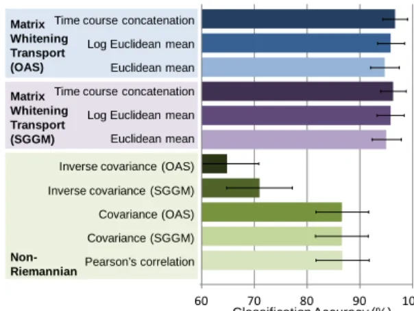
Fig. 5. Riemannian vs. non-Riemannian approaches. Four state classification accuracy displayed. By reducing correlations between connectivity features using the proposed transport, significantly higher accuracy was obtained.

Using Pearson’s correlation resulted in a classification accuracy of 87% (Fig. 5), and similar accuracy was obtained by regularizing the Pearson’s correlation estimates with OAS and SGGM. With inverse covariance, a dramatic drop in classification accuracy was observed, and thus was not further pursued in the transport comparisons. Projecting the state covariance estimates onto the tangent space using the proposed matrix whitening transport achieved 94% to 97% classification accuracy. Also, lower variability in accuracy across subsamples was observed. Since regularizing the covariance estimates with OAS and SGGM without projection did not improve classification performance, we could safely attribute the gain in accuracy with our approach to its correlation reduction property on connectivity features. This gain also suggests that the closeness assumption between the state and base covariance estimates was likely met. The choice of covariance estimation method, i.e. using SGGM or OAS, only mildly affected the accuracy. Thus, OAS would be preferred for its computational efficiency, i.e. OAS only involves one matrix multiplication and a few scalar additions and divisions. The choice of mean covariance estimation method did have a minor impact in absolute terms with mean covariance estimated from time courses concatenated across conditions outperforming Euclidean and Log Euclidean mean. We speculate that the increased number of time samples by concatenating the time courses improves the conditioning of the estimation, whereas Euclidean and Log Euclidean mean amount to averaging poorly estimated sample covariance matrices that are strongly regularized by OAS and SGGM.

In addition to the presented experiment, we applied our proposed transport to datasets from three other studies. One of

60 70 80 90 100

1

Euclidean mean Log Euclidean mean Time course concatenation

Matrix Whitening Transport (OAS)

Euclidean mean Log Euclidean mean Time course concatenation

Matrix Whitening Transport (SGGM) Classification Accuracy (%) Pearson’s correlation Covariance (SGGM) Covariance (OAS) Non-Riemannian

Inverse covariance (OAS) Inverse covariance (SGGM)

the studies involved 51 healthy subjects lying at rest and were scanned twice, with a 24 min memory task between the two scans [8]. The accuracy achieved in classifying whether a connectivity pattern corresponds to before or after the memory task was 98% with our approach, whereas using Pearson’s correlation as features obtained an accuracy of 76%. Our results thus indicate that even within a short duration of 24 min, detectable functional rewiring appears to be present. We also applied our approach to data in which 57 Parkinson’s disease patients lying at rest were scanned twice, once off medication and once on medication. Our approach achieved an accuracy of 97%, whereas using Pearson’s correlation obtained an accuracy of 51%. With this level of accuracy, one can envision using our classifier to help evaluate the effectiveness of medication, i.e. if a patient on medication is classified as off medication, the medication might not have been very effective. Both set of results demonstrate the suitability of our approach for longitudinal studies. Further, we applied our approach to study mood disorders. Classifying whether a subject was in a happy or ruminative state, an accuracy of 89% was achieved, whereas using Pearson’s correlation obtained an accuracy of 53% [6].

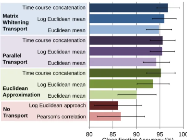
Fig. 6. Covariance transport comparison. Only results with OAS used for state and base covariance estimation shown. For the same mean covariance estimation method, the proposed matrix whitening transport was found to achieve the highest classification accuracy in absolute terms.

Comparing the various transports with covariance estimation performed using OAS (Fig. 6), projecting the state covariance estimates onto the tangent space at the identity matrix without transporting, i.e. the Log Euclidean approach [15], resulted in the lowest classification accuracy of 86%, which was lower than simply using Pearson’s correlation. In contrast, the various transports all achieved accuracy above 90%, suggesting the necessity of transporting prior to projection onto the tangent space. Using the Euclidean approximation of the proposed matrix whitening transport obtained accuracy of 90% to 95%, whereas using parallel transport attained accuracy of 94% to 96%, similar to the accuracy achieved with the proposed transport. Thus, our results demonstrate that using manifold operations to properly account for the structure of the space of covariance matrices is beneficial. Also, the variability in accuracy with respect to the mean covariance estimation method was notably lower

compared to the Euclidean approximation. For the same mean covariance estimation method, the proposed matrix whitening transport slightly outperformed parallel transport. The computational time to transport all 96 covariance matrices with the proposed transport is about 10 seconds for a single-core 2.65GHz machine, whereas parallel transport (for one-step transport) requires a bit over a minute. Thus, from a computational standpoint, the proposed transport would be preferred. We highlight that not any means of removing the positive semidefinite constraint provides such accuracy gain, as evident from the lower accuracy with the Log Euclidean approach compared to the proposed transport. Moreover, linearly removing the commonalities across conditions using the Euclidean approximation, though resulted in some improvements, was inferior to the proposed transport. Thus, our results suggest that it is the combination of both removing the positive semidefinite constraint as well as isolating the distinctive connectivity attributes of the different brain states by nonlinearly removing their subject-specific commonalities (which is part of the process of the proposed transport) that provided the observed accuracy gain. We further note that by introducing the notion of matrix whitening transport, we are no longer bounded to use a common group base covariance for all subjects as in [9]. Since a subject-specific base covariance is more similar to each subject’s state covariance matrices than a group covariance due to inter-subject variability, the closeness assumption for projection would be better fulfilled. To confirm this intuition, we applied the same Riemannian approach but with the Log Euclidean mean across training subjects and conditions used as the common base covariance. The attained accuracy was 84%, which demonstrates the advantage of using subject-specific base covariance. Lastly, using SGGM for covariance estimation led to similar accuracy and exactly the same trend with the proposed transport outperforming the others in absolute terms.

Maintaining continual, self-driven tasks for 10 min could be difficult. We thus performed the same analysis on shorten time courses by taking the first 2 min, 5 min, and 8 min (Fig. 7).

Fig. 7. Effects of fewer time samples. Only results with covariance estimated using OAS and base covariance computed from concatenated time course shown. PC = Pearson’s correlation (pink), LE = Log Euclidean (red), EA = Euclidean approximation (green), PT = parallel transport (purple), and WT = Whitening transport (blue). The trend that the proposed matrix whitening transport outperforming the contrasted methods was preserved.

80 85 90 95 100

1

Euclidean mean Log Euclidean mean Time course concatenation

Matrix Whitening Transport

Euclidean mean Log Euclidean mean Time course concatenation

Parallel Transport

Euclidean mean Log Euclidean mean Time course concatenation

Euclidean Approximation

Pearson’s correlation Log Euclidean approach

No Transport Classification Accuracy (%) 75 80 85 90 95 100 1 2 3 4 Cla ssif ic at io n Ac cu ra cy (% ) 2 5 8 10

Length of region time courses (min)

WT

EA PT

LE

Overall, the proposed transport achieved the highest accuracy in absolute terms. Our results thus show that the presented classification approach is just as applicable for lower sample-to-feature ratios. The accuracy seems higher between 5 min to 8 min. We speculate the lower accuracy with 10 min was due to fatigue and more mind wandering. Hence, although increasing the number of time samples should improve covariance estimation, some of the time samples might not reflect the brain state that the subjects were asked to engage in. Also, the standard deviation of the classification accuracy (not displayed to avoid clutter) gradually increased by ~1.5% from 10 min to 2 min for all contrasted methods.

To identify significantly discriminative brain connections, we applied our proposed non-parametric scheme (Section II-G) on classifier weights learned with all subjects’ dCc(s) as

features. We present here only results for dCc(s) estimated

using the proposed matrix whitening transport with covariance estimated with OAS and mean covariance computed from concatenated time courses. Statistical significance is declared at a p-value threshold of 0.01 with multiple comparisons implicitly corrected for using maximum statistics [27].

(a) Memory vs. rest (b) Subtraction vs. rest Fig. 8. Significant discriminative brain connections. DLPFC = dorsolateral prefrontal cortex, mPFC = medial prefrontal cortex, PCC = posterior cingulate cortex, ACC = anterior cingulated cortex, SPL = superior parietal lobule. Red arrows indicate significant connections also detected with paired t-test.

For memory versus rest (Fig. 8(a)), a number of significant connections between memory-relevant brain regions, such as posterior cingulate cortex (PCC), medial prefrontal cortex (mPFC), dorsal lateral prefrontal cortex (DLPFC), thalamus, and middle temporal gyrus (MTG) were found. PCC is a key hub in the default-mode network (DMN) [28] and is targeted early in the course of Alzheimer’s disease, i.e. the quintessential disorder of memory impairment [29]. The mPFC is also part of the DMN, and its connections to PCC have been shown to differentiate memory tasks from resting [30]. The DLPFC plays a major role in working memory [31]. The thalamus is critical for episodic memory [32] and the left MTG is associated with semantic memory [33]. Thus, the detected connections match well with what one would expect for a task that involves recalling events of the day.

For subtraction versus rest (Fig. 8(b)), we found significant inter-connections mainly between the angular gyrus, DLPFC, superior parietal lobule (SPL), anterior cingulated cortex

(ACC), mPFC, and precuneus. The angular gyrus is known to be involved in number processing and lesions to this region would result in dyscalculia [34]. The DLPFC and SPL are typical areas responsible for working memory [35], a likely cognitive component for serial subtraction given the need to constantly update the subtraction problem. The ACC plays a major role in performance evaluation and is evoked upon errors during task performance [36]. The mPFC and precuneus are also widely observed in mental arithmetic tasks due to their involvement in work memory [37]. The identified connections thus conform to our expectation. Note that we displayed significant connections at a more stringent p-value threshold of 0.001 in Fig. 8(b) to avoid cluttering the plot. For singing versus rest, we found significant inter-connections between the insula, sensorimotor cortex, ACC, mPFC, and MTG, which are involved with the motor and emotional processing pertinent to imagined singing [38].

We highlight here several observations. First, no significant connections were found for any of the three contrasts using pure permutation testing on classifier weights, thus illustrating superior detection sensitivity with our proposed scheme for discriminative connection identification. Second, since using Log Euclidean mean as base covariance estimates resulted in similar classification performance as using mean covariance estimated from concatenated time courses, we tested our proposed scheme on dCc(s) estimated with Log Euclidean

mean. The detected brain connections were found to be a subset of those obtained with time course concatenation for the same p-value threshold. Third, using SGGM for covariance estimation resulted in similar connections found with slightly higher detection sensitivity. Lastly, to contrast our proposed scheme against the more standard maximum likelihood approach, we performed paired t-test on dCc(s).

Using maximum statistics to correct for multiple comparisons [27], the found connections (red arrows in Fig. 8) were a subset of those detected by our proposed scheme, thus demonstrating consistency in results between two vastly different approaches.

Noteworthy is that our strategy for dealing with correlated features is quite different from many feature selection methods. Most feature selection methods try to find a subset of uncorrelated features, but the feature selected from each correlated set is often arbitrary. Instead, our strategy is to retain all features but reduce their inter-correlations. This strategy is especially advantageous for significant feature detection, since multiple (originally) correlated features might be jointly relevant. A related note is the interpretation of the elements of dCc(s). Analogous to how partial correlation is

another definition of connectivity that also involves nonlinear operations applied to the covariance matrices (i.e. matrix inversion followed by normalization), dCc(s) should be

viewed as just another definition. Under the affine invariant framework [10], there is no ambiguity regarding the interpretation of the (i, j)th element of dCc(s) as an estimate of

the connectivity between regions i and j, but the definition of connectivity under this framework is different from Pearson’s correlation and partial correlation.

Right Left mPFC PCC PCC DLPFC Middle Temporal Gyrus Thalamus mPFC Precuneus ACC Angular gyrus SPL DLPFC Angular gyrus SPL Right Left

V. CONCLUSIONS

We proposed a new functional connectivity-based approach for decoding more naturalistic, subject-driven brain states. By using manifold operations to reduce the correlations between connectivity features, significantly higher classification accuracy was obtained compared to the more standard approach of directly using Pearson’s correlation as features, which are inherently inter-related. Also, higher detection sensitivity was shown with our proposed discriminative connection identification scheme compared to conventional permutation testing. The overall framework thus provides both classification accuracy and result interpretability. Based on our results, we recommend using matrix whitening transport on OAS covariance estimates and mean covariance estimated from concatenated time courses to execute the presented Riemannian approach.

REFERENCES

[1] K. A. Norman, S. M. Polyn, G. J. Detre, and J. V. Haxby, "Beyond mind-reading: Multi-voxel pattern analysis of fMRI data," Trends Cogn. Sci., vol. 10, pp. 424-430, 2006.

[2] J. D. Haynes and G. Rees, "Decoding mental states from brain activity in humans," Nat. Rev. Neurosci., vol. 7, pp. 523-534, 2006.

[3] W. James, The principles of psychology. New York, Holt and Company, 1918.

[4] W. Shirer, S. Ryali, E. Rykhlevskaia, V. Menon, and M. Greicius, "Decoding subject-driven cognitive states with whole-brain connectivity patterns," Cereb. Cortex, vol. 22, pp. 158-165, 2012.

[5] J. Richiardi, H. Eryilmaz, S. Schwartz, P. Vuilleumier, and D. Van De Ville, "Decoding brain states from fMRI connectivity graphs," NeuroImage, vol. 56, pp. 616-626, 2011.

[6] A.C. Milazzo, B. Ng, H. Jiang, W. Shirer, G. Varoquaux, J. B. Poline, B. Thirion, and M. D. Greicius, "Identification of mood-relevant brain connections using a continuous, subject-driven rumination paradigm," Cereb. Cortex, 2014. (in press)

[7] F. X. Castellanos, A. Di Martino, R. C. Craddock, A. D. Mehta, and M. P. Milham, "Clinical applications of the functional connectome," NeuroImage, vol. 80, pp. 527-540, 2013.

[8] B. Ng, M. Dressler, G. Varoquaux, J. B. Poline, M. Greicius, and B. Thirion, "Transport on Riemannian manifold for functional connectivity-based classification," in Int. Conf. Medical Image Computing and Computer-Assisted Intervention, Boston, M.A., 2014, pp. 405-412. [9] G. Varoquaux, F. Baronnet, A. Kleinschmidt, P. Fillard, and B. Thirion,

"Detection of brain functional connectivity difference in post-stroke patients using group-level covariance modeling," in Int. Conf. Medical Image Computing and Computer-Assisted Intervention, Beijing, China, 2010, pp. 200-208.

[10] X. Pennec, P. Fillard, and N. Ayache, "A Riemannian framework for tensor computing," Int. J. Computer Vision, vol. 66, pp. 41-66, 2006. [11] L. Toloşi and T. Lengauer, "Classification with correlated features:

unreliability of feature ranking and solutions," Bioinformatics, vol. 27, pp. 1986-1994, 2011.

[12] J. E. Desmond and G. H. Glover, "Estimating sample size in functional MRI (fMRI) neuroimaging studies: statistical power analyses," J. Neurosci. Methods, vol. 118, pp. 115-128, 2002.

[13] Y. Chen, A. Wiesel, Y. C. Eldar, and A. O. Hero, "Shrinkage algorithms for MMSE covariance estimation," IEEE Trans. Sig. Proc., vol. 58, pp. 5016-5029, 2010.

[14] C. J. Hsieh, M. A. Sustik, P. Ravikumar, and I. S. Dhillon, "Sparse inverse covariance matrix estimation using quadratic approximation," in Int. Conf. Advances in Neural Information Processing Systems, Granada, Spain, 2011, pp. 2330-2338.

[15] V. Arsigny, P. Fillard, X. Pennec, and N. Ayache, "Fast and simple calculus on tensors in the Log-Euclidean framework," in Int. Conf. Medical Image Computing and Computer-Assisted Intervention, Palm Springs, C.A., 2005, pp. 115-122.

[16] M. Knebelman, "Spaces of relative parallelism," Ann. Mathematics, vol. 53, pp. 387-399, 1951.

[17] S. Hauberg, F. Lauze, and K. S. Pedersen, "Unscented Kalman Filtering on Riemannian Manifolds," J. Math. Imaging & Vision, vol. 46, pp. 103-120, 2013.

[18] A. Schild, "Tearing geometry to pieces: More on conformal geometry," Unpublished lecture, Princeton Univesity relativity seminar, 1970. [19] C.W. Misner, K.S. Thorne, and J. A. Wheeler, Gravitation. Freeman,

New York, 1973.

[20] M. Lorenzi, N. Ayache, and X. Pennec, "Schild’s ladder for the parallel transport of deformations in time series of images," in Int. Conf. Information Processing in Medical Imaging, Kloster Irsee, Germany, 2011, pp. 463-474.

[21] P. Bühlmann, "Statistical significance in high-dimensional linear models," Bernoulli, vol. 19, pp. 1212-1242, 2013.

[22] A. Javanmard and A. Montanari, "Confidence intervals and hypothesis testing for high-dimensional regression," J. Machine Learning Research, vol. 15, pp. 2869-2909, 2014.

[23] C.W. Hsu and C.-J. Lin, "A comparison of methods for multiclass support vector machines," IEEE Trans. Neural Networks, vol. 13, pp. 415-425, 2002.

[24] B. Ng, G. Varoquaux, J. B. Poline, and B. Thirion, "A novel sparse graphical approach for multimodal brain connectivity inference," in Int. Conf. Medical Image Computing and Computer-Assisted Intervention, Nice, France, 2012, pp. 707-714.

[25] M. D. Fox and M. E. Raichle, "Spontaneous fluctuations in brain activity observed with functional magnetic resonance imaging," Nat. Rev. Neurosci., vol. 8, pp. 700-711, 2007.

[26] P. T. Fletcher and S. Joshi, "Riemannian geometry for the statistical analysis of diffusion tensor data," Sig. Processing, vol. 87, pp. 250-262, 2007.

[27] T. Nichols and S. Hayasaka, "Controlling the familywise error rate in functional neuroimaging: a comparative review," Stat. Meth. Med. Research, vol. 12, pp. 419-446, 2003.

[28] P. Hagmann, L. Cammoun, X. Gigandet, R. Meuli, C. J. Honey, V. J. Wedeen, and O. Sporns, "Mapping the structural core of human cerebral cortex," PLoS Biology, vol. 6, p. e159, 2008.

[29] M. D. Greicius, G. Srivastava, A. L. Reiss, and V. Menon, "Default-mode network activity distinguishes Alzheimer's disease from healthy aging: evidence from functional MRI," Proc. Natl. Acad. Sci. U.S.A., vol. 101, pp. 4637-4642, 2004.

[30] M. D. Greicius, B. Krasnow, A. L. Reiss, and V. Menon, "Functional connectivity in the resting brain: A network analysis of the default mode hypothesis," Proc. Natl. Acad. Sci. U.S.A., vol. 100, p. 253-258, 2003. [31] M. Petrides, "The role of the mid-dorsolateral prefrontal cortex in

working memory," Exp. Brain Res., vol. 133, pp. 44-54, 2000.

[32] J. P. Aggleton, S. M. O’Mara, S. D. Vann, N. F. Wright, M. Tsanov, and J. T. Erichsen, "Hippocampal–anterior thalamic pathways for memory: uncovering a network of direct and indirect actions," Eur. J. Neurosci., vol. 31, pp. 2292-2307, 2010.

[33] J. R. Binder, R. H. Desai, W. W. Graves, and L. L. Conant, "Where is the semantic system? A critical review and meta-analysis of 120 functional neuroimaging studies," Cereb. Cortex, vol. 19, pp. 2767-2796, 2009.

[34] E. Rusconi, P. Pinel, E. Eger, D. LeBihan, B. Thirion, S. Dehaene, and A. Kleinschmidt, "A disconnection account of Gerstmann syndrome: functional neuroanatomy evidence," Ann. Neurology, vol. 66, pp. 654-662, 2009.

[35] S. Dehaene, E. Spelke, P. Pinel, R. Stanescu, and S. Tsivkin, "Sources of mathematical thinking: Behavioral and brain-imaging evidence," Science, vol. 284, pp. 970-974, 1999.

[36] F. E. Polli, J. J. Barton, M. S. Cain, K. N. Thakkar, S. L. Rauch, and D. S. Manoach, "Rostral and dorsal anterior cingulate cortex make dissociable contributions during antisaccade error commission," Proc. Natl. Acad. Sci. U.S.A., vol. 102, pp. 15700-15705, 2005.

[37] T. Fehr, C. Code, and M. Herrmann, "Common brain regions underlying different arithmetic operations as revealed by conjunct fMRI–BOLD activation," Brain Research, vol. 1172, pp. 93-102, 2007.

[38] B. Kleber, N. Birbaumer, R. Veit, T. Trevorrow, and M. Lotze, "Overt and imagined singing of an Italian aria," NeuroImage, vol. 36, pp. 889-900, 2007.