Material Classification from Imprecise Chemical Composition : Probabilistic vs Possibilistic Approach

HAL Id: cea-01992290

https://hal-cea.archives-ouvertes.fr/cea-01992290

HAL is a multi-disciplinary open access

archive for the deposit and dissemination of sci-entific research documents, whether they are pub-lished or not. The documents may come from teaching and research institutions in France or

L’archive ouverte pluridisciplinaire HAL, est destinée au dépôt et à la diffusion de documents scientifiques de niveau recherche, publiés ou non, émanant des établissements d’enseignement et de recherche français ou étrangers, des laboratoires

Material Classification from Imprecise Chemical

Composition : Probabilistic vs Possibilistic Approach

Arnaud Grivet Sébert, Jean-Philippe Poli

To cite this version:

Arnaud Grivet Sébert, Jean-Philippe Poli. Material Classification from Imprecise Chemical Composi-tion : Probabilistic vs Possibilistic Approach. 2018 IEEE InternaComposi-tional Conference on Fuzzy Systems (FUZZ-IEEE), Jul 2018, Rio de Janeiro, Brazil. pp.8491485, �10.1109/FUZZ-IEEE.2018.8491485�. �cea-01992290�

Material Classification from Imprecise Chemical

Composition : Probabilistic vs Possibilistic

Approach

Arnaud Grivet S´ebert and Jean-Philippe Poli CEA, LIST

Data Analysis and System Intelligence Laboratory Gif-sur-Yvette, France

{arnaud.grivet.sebert,jean-philippe.poli}@cea.fr 2018

Abstract

In this paper we propose a method of explainable material classi-fication from imprecise chemical compositions. The problem of clas-sification from imprecise data is addressed with a fuzzy decision tree whose terms are learned by a clustering algorithm. We deduce fuzzy rules from the tree, which will provide a justification of the result of the classification. Two opposed approaches are compared : the prob-abilistic approach and the possibilistic approach.

1

Introduction

Customs and ports security is a major issue in Europe. Indeed, many illegal or dangerous substances such as drugs, weapons, explosives pass through customs. Unfortunately, systematic container inspections are impossible in practice because of the cost and time that would be required. The vol-umes passing daily through the major European ports such as Rotterdam, Antwerp or Hamburg are indeed enormous: for example, 461.2 million tons of goods passed through the port of Rotterdam in 2016.

Our work is part of the C-BORD European project which aims at de-termining the content of containers using various technologies. One of these technologies uses tagged neutrons, which allows to obtain the chemical com-position of a volume of the container. From this chemical comcom-position, we want to determine the materials present in this volume of the container. In order to bring more credibility to the final software used by the customs officers, we will also provide a justification for this classification. Fuzzy rules allow to avoid the “black box” effect since customs officers have access to

a real explanation of the classification made by the software, and close to natural language : “the container may contain drug (confidence degree : x) because the quantity of carbon is high, the quantity of nitrogen is low and the quantity of oxygen is medium” for instance.

The proportions are obtained by different treatments that are beyond our control. Thus, the input data are imprecise and are accompanied by a measure of this inaccuracy. Fuzzy logic thus seems appropriate for the exploitation of such data.

Given the time required and the authorizations needed to use a neu-tron generator, we will have a small learning data set, even if all classes of relevant materials will obviously be represented. The idea is therefore to use fuzzy decision trees [4], which have been applied successfully on var-ious classification problems [1, 13]. The scarcity of training data and the intrinsic inaccuracy due to the preprocessing preclude conventional statisti-cal learning approaches such as neural networks, SVM, etc. which also do not provide an explanation to users.

In this article, we adapt to imprecise data the classic two-step workflow consisting in using clustering methods to create relevant terms from data and then in building a decision tree to get either a probabilistic or a possibilistic classifier. We propose a comparison of these two approaches, as some authors did for other applied problems [8], [12].

The paper is structured as follows: section 2 describes the context of the application that motivates this work. Then, section 3 describes the method to induce rules from imprecise data. Section 4 presents the results of the different experiments we conducted. Finally, section 5 draws the conclusions of this paper.

2

Application context

2.1 Neutron inspection for container digging

The H2020 project C-BORD (effective Container inspection at BORDer control points) aims at securing borders by exploiting different technologies: e-noses, X-rays, photo-fission and tagged neutrons. The goal is to detect dangerous (explosives, nuclear materials, ...) or illicit (drugs, contraband, ...) substances in containers.

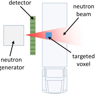
In this paper, we focus on the use of tagged neutron and material classi-fication. As shown in fig. 1, we use a device which produces a neutron beam to focus on a certain voxel (i.e. a volume) of the container. The neutrons interact with the nuclei of the atoms contained in the voxel, producing new particles that can be detected by the matrix sensors which are positioned on the side of the container. These particles are thus characteristic of the atoms encountered in the examined voxel.

neutron

generator

detector

neutron

beam

targeted

voxel

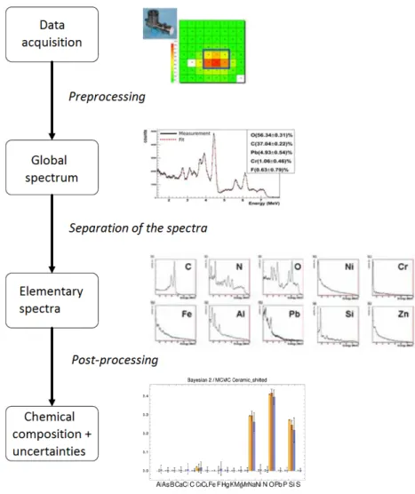
Figure 2: Workflow to get chemical composition assessment from raw data acquisition

The processing of the raw data is not the topic of this article but we quickly describe the principle in fig. 2. After different pretreatments, a global spectrum is obtained. In comparison with the characteristic spectra of each of the studied atoms, this spectrum is decomposed into individual spectra by a Bayesian process which makes it possible to deduce the chemical composition of the voxel, expressed in percentages. This process is based on simulation and we can easily get the mean and the standard deviation for each proportion in order to characterize the inaccuracy of the reconstruction. Fig. 3 shows the result of these treatments for an exposure to ceramics, and in which the inaccuracy is represented by “box plots”.

Figure 3: Chemical composition obtained from ceramics simulation Our work consists in exploiting this information in order to recognize the materials contained in the voxel.

2.2 Previous work

We barely found some articles concerning the use of tagged neutrons to characterize materials. This can be explained by several difficulties.

First, data are scarce because few acquisition campaigns can be con-ducted. That also explains why few papers address the recognition of mate-rials from their chemical composition. Then, the inaccuracy of the chemical composition makes the task difficult for conventional statistical models. Fi-nally, a not insignificant difficulty is that the device is insensitive to hydrogen atoms, and thus some materials cannot be distinguished.

For these reasons, previous works proposed visual analytics methods to represent the content of the voxels. In [2], the authors proposed a Voronoi diagram to highlight the proximity, in terms of chemical composition, of the current voxel with voxels previously inspected and whose content is known

Figure 4: Screenshots of the different visualizations introduced in [2] (see figure 4). Thus, it is not a question of recognizing the materials inside the container but of displaying visually close and known containers in order to deduce the contents.

This approach has the advantage of not requiring learning or parametriza-tion since it relies on the manual selecparametriza-tion of a neighborhood. In figure 4, we can also see two classical representations that have been used in conjunc-tion with this method. These are projecconjunc-tions of the current voxel onto two triangles:

ˆ the “materials triangle” indicates the proximity of the voxel with met-als, ceramics and organic materials;

ˆ the “alert triangle” presents the ratios between carbon, nitrogen and oxygen and is useful to recognize organic materials (even if the hydro-gen is not detected).

The latter triangle helps to distinguish between drugs and explosives. The main drawback of the visual analytics approach is that the operator must be able to interpret the different representations himself.

In practice, the mastering of these representations, particularly the Voronoi graph, can be difficult for operators who are not familiar with these visual-ization techniques. As part of the C-BORD project, we want to go further and propose a list of materials, and an explanation of the decision. It is

to overcome these different difficulties that we want to use a fuzzy expert system.

3

Fuzzy material classification

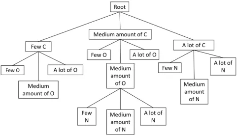
To solve the classification problem we build a fuzzy decision tree [4] from which fuzzy rules are extracted to provide the end-user with a justification of the result. Each node of the tree is split into child nodes by an attribute, i.e. a chemical element. The child nodes correspond to fuzzy terms induced by a strong partition of the domain of the chemical ratios, namely [0, 100] since they are percentages. If no pruning is performed, the tree has a maximal depth equal to the number of chemical elements used as attributes for the classification. An example of a tree is shown in fig. 5.

Root Few C Medium amount of C A lot of C Few N Medium amount of N A lot of N Few N Medium _amount of N A lot of N Few O Medium amount of O A lot of O Few O Medium amount of O A lot of O

Figure 5: Fuzzy tree for material classification

The imprecise inputs are modeled as either probability or possibility distributions. In the probabilistic case, the distributions are Gaussian dis-tributions normalized so that their integral on the domain of the input data, namely [0, 100], equals 1. In the possibilistic case, we tested triangular and Gaussian distributions normalized so that their maximum value is 1.

We chose to learn fuzzy terms and to build the decision tree in two separate phases.

3.1 Fuzzy terms learning

Among the various methods we tested, the best methods to learn linguistic terms turned out to be clustering techniques. We describe hereafter the adaptations of two clustering algorithms.

3.1.1 Measures of dissimilarity

We modified these algorithms using a dissimilarity adapted to imprecise data. We consider the following dissimilarity for the probabilistic case :

d(x, y) = 1 − Z b

a

min(fx(t), fy(t))dt (1)

where fx and fy are the densities of the distributions representing the data

x and y, a and b are the bounds of the definition domain of the data, 0 and 100 in our case. This dissimilarity is actually a distance for continuous probability distributions but we will not prove it here for reasons of space.

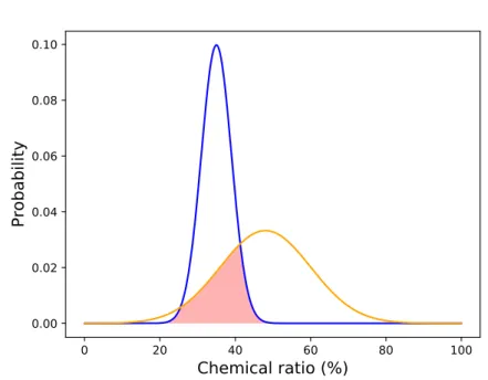
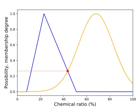
In the possibilistic case, the integral is replaced by the max. Fig. 6 shows the area corresponding to the associated similarityRb

amin(fx(t), fy(t))dt

between two Gaussian probability distributions, drawn in red.

0 20 40 60 80 100

Chemical ratio (%)

Probability

Figure 6: Similarity between two imprecise data - probabilistic modeling We tested several algorithms and decided to study more thoroughly medoids and affinity propagation because they gave better results than k-means and DBSCAN in particular. K-k-means implies to compute the dis-tance between a data input and a centroid, which is a single point randomly chosen and hence cannot be modeled as an imprecise datum. Unable to use the previously defined dissimilarity, we used asymmetric dissimilarities (in the probabilistic case for example, the integral of the distance between the centroid and the moving point of the imprecise distribution). This incom-patibility between the imprecise inputs and the single-point centroids might

explain the poorer results. Using DBSCAN, we often obtained a very small number of clusters because the data distribution is quite continuous along the domain [0, 100]. Since DBSCAN works by analyzing the neighborhood of each data point, the absence of clear gaps in the data distribution prevents DBSCAN from splitting the data set.

3.1.2 K-medoids

We adapted k-medoids algorithm [11] to cluster the imprecise data by substi-tuting the traditional Euclidean distance by the dissimilarity defined above. This well-known algorithm takes the number n of clusters as a parameter. It randomly chooses n objects from the dataset to be the initial centers of the clusters and the other objects are assigned to the closest center. In each cluster, the object minimizing the sum of the distances to the other objects is set as the new center. Then the algorithm alternatively updates the sets belonging to each cluster and the centers until convergence. The output is the best result over several initial random configurations.

3.1.3 Affinity propagation

We also tested the affinity propagation algorithm [6]. In this algorithm, every data point is a potential cluster exemplar. A distribution of similarity for each pair of points is given as an input. Another parameter, a real called preference, is used to control the number of clusters.

The data points send “messages” to each other. A data point i sends to a data point k the responsibility r(i, k) which represents how much i is likely to be in a cluster whose exemplar is k. k sends to i the availability a(i, k) which represents how much k is available for i to be in its cluster. The exemplars are the points i such that r(i, i) + a(i, i) > 0 and a data point is assigned to the closest exemplar according to the given similarity. The responsibilities depend on the similarity distribution. Besides, the re-sponsibilities are function of the availabilities and conversely. The algorithm successively updates the responsibilities and availabilities until the clusters converge. We implemented this algorithm using the similarity associated with the dissimilarity defined in 1.

3.1.4 From clusters to membership functions

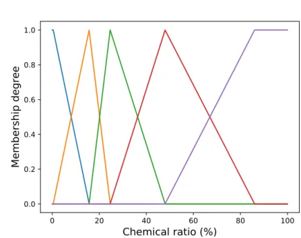
From each cluster we deduce a triangular fuzzy term whose top, of value 1, is set at the center of the cluster. The slopes are induced by the other terms’ tops under the strong partition constraint. The extreme sets are slightly different : they are right-angled trapezoids whose flat part ends at the bound of the domain. We can see an example of a five-set partition in fig. 7. More complex term shapes (trapezoids, pentagons) reduce the performance and even the accuracy in some cases.

0 20 40 60 80 100

Chemical ratio (%)

Membership degree

Figure 7: Five learned fuzzy sets

3.2 Construction of the fuzzy decision tree

3.2.1 Probabilistic approach

To build the fuzzy decision tree, we also need to adapt to imprecise data the definition of the membership degrees to the linguistic terms. In [5] and [15], the authors proposed integration techniques to deal with relations between uncertain data and crisp terms. We generalized these techniques to imprecise data and fuzzy terms.

Given f the density of the probability distribution representing the im-precision associated with the proportion of an element e in an example x, and µv(t) the membership degree of the value t to the fuzzy term v, the

membership degree of the imprecise example x to the fuzzy term v is : ˜

µv(x) =

Z 100

0

f (t)µv(t)dt (2)

This definition is illustrated in fig. 8 where the imprecision distribution is dilated 10 times for a better visibility.

The membership degree of an imprecise input x to a node n is defined as the product of the membership degrees to the linguistic terms associated with the ascendants of n, including n :

dn(x) =

Y

n0_∈A(n)

˜

0 20 40 60 80 100

Chemical ratio (%)

Figure 8: Membership degree of an imprecise datum to a linguistic term -probabilistic modeling

where, for all node n0 , vn0 is the linguistic term associated with n0, and A(n)

is the set of the ascendants of n, including n. By convention, the degree of any input to the root is equal to 11_.

Using this definition, we can compute the fuzzy entropy, inspired from [14], which is the criterion to select which attribute will be used to split a node. We consider the “fuzzy frequency” of a class c in a node n :

f rc/n=

P

x∈Tr∩cdn(x)

P

x∈Trdn(x)

where Tr is the training set. We also define the “membership frequency” of the examples to the node n :

f rn= P x∈Trdn(x) P m∈S P x∈Trdm(x)

where S is the set of the sibling nodes of n, including n.

The fuzzy entropy, according to an element e, used at a node N whose set of children is noted Chil(N ), these nodes corresponding to each fuzzy term relative to e, is then defined as :

E(N ) = − X n∈Chil(N ) f rn X c∈C f rc/n× log2(f rc/n) 1

Any other non negative real d0 would lead to the same results since it would only

where C is the set of the classes of the problem.

Each node n of the tree is split in child nodes regarding the linguistic terms corresponding to the chemical element which minimizes the entropy, thus maximizing the entropy gain G(n) = E(N ) − E(n), N being the father of n. This node splitting is processed until one of the following stopping criteria is reached :

ˆ All the attributes have been used splitting the ascendants of the cur-rent node.

ˆ The sum of the membership degrees to the current node is less than a threshold fixed in advance.

ˆ The entropy gain is less than another threshold fixed in advance. 3.2.2 Possibilistic approach

The definition 2 is replaced by : ˜

µv(x) = max

06t6100(min(f (t), µv(t))) (4)

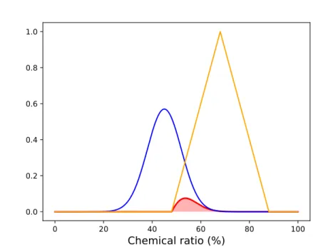
where the possibilistic norms max and min are used. Fig. 9 illustrates this definition in the case of a Gaussian modeling of the input datum. Note that this definition coincides with the possibilistic similarity defined in 3.1.1, applied to a datum and a linguistic term.

The membership degree of an imprecise input x to a node n is defined as the minimum of the membership degrees to the linguistic terms associated with the ascendants of n, including n :

dn(x) = min

N ∈A(n)µ˜vN(x) (5)

where, for all node N , vN is the linguistic term associated with N , and

A(n) is the set of the ascendants of n, including n.

We replaced the entropy by another splitting criterion, the non-specificity, proposed in [7]. We consider an ordered discrete possibility distribution (πi)16i6m such that ∀i ∈ [|1, m − 1|], πi > πi+1 and π1 = 1. We also note

πm+1 = 0. The measure of non-specificity, called U-uncertainty is defined

as follows :

U (π) =

m

X

i=2

(πi− πi+1)log2(i)

In our case, π is the possibility distribution of the classes in the current node : for every class c in C we note

π_c/n=

P

x∈Tr∩cdn(x)

maxc0_∈CP

0 20 40 60 80 100

Chemical ratio (%)

Possibility, membership degree

Figure 9: Membership degree of an imprecise datum to a linguistic term -possibilistic modeling

We then sort (πc/n)c∈C in the decreasing order and compute the

non-specificity using the formula above.

The stopping criteria are the same as in the probabilistic framework, the entropy gain being replaced by the non-specificity gain NSG(n) = U (N ) − U (n), where N is the father of the node n.

To avoid the bias due to the varying number of linguistic terms of the attributes, we decided, inspiring from [10], to normalize the non-specificity gain by the SplitInfo(n) = −P

n0_∈Chil(n)f r_n0× log₂(f r_n0) which is actually

the potential fuzzy entropy generated by splitting the node n, ignoring the classes of the samples.

3.3 Rule generation

While the tree is being built, the fuzzy frequencies f rc/l of every class c in

every leaf l are computed and stored in memory. We then obtain, for each leaf, |C| rules - |C| being the number of classes of the problem -, weighted by the associated fuzzy frequency which corresponds to the “certainty factor”, as defined in [3]. For instance, in fig. 5, the leaf on the extreme right will induce the rules “if there is a lot of carbon and a lot of nitrogen, then the object is in class c”, for all c in C.

3.4 Recognition of input test data

As both training and test data are imprecise, for every new test sample x, we compute the membership degree of x to every leaf of the tree using the very same definition as in the training phase (3 or 5). Given a class c, this membership degree is then conjugated by the appropriate T-norm with the certainty factor of each rule whose consequent is c and the results are summed up using the weighted voting method [9] to obtain the confidence degree of the proposition x ∈ c :

conf(x ∈ c) =X

l∈L

T (f r_c/l, dl(x))

where L is the set of the leaves of the tree and T is the probabilistic (resp. possibilistic) T-norm × (resp. min). We finally deduce the distribution of the classes for the input x normalizing the confidence degrees. In the probability case, we then have :

∀c ∈ C, px(c) =

conf(x ∈ c) P

c0_∈Cconf(x ∈ c0)

(6) and in the possibilitic case :

∀c ∈ C, π_x(c) = conf(x ∈ c)

maxc0_∈Cconf(x ∈ c0) (7)

4

Experiments

4.1 Data simulation

We decided to test several methods on simulated data while waiting for real data. To do so, we refer to the molecular formulæ of the different materials - the classes of the problem. For each material m and each element e, we deduce from the formula of m the stoichiometric percentage of e in m. This percentage p is used as a reference around which we randomly and in an uniform way pick a value v in the interval [p − p ×₁₀₀DI, p + p ×₁₀₀DI]. The span of this interval is proportional to p and to a parameter DI we call “degree of imprecision”, used to control the level of imprecision of the generated data. We then generate a random standard deviation σ via a normal distribution of mean p₂× DI

100 and standard deviation p 4×

DI

100. The tuple (v, σ) constitutes

an imprecise datum.

We ran the experiments with data generated from the molecular formulæ of seventeen explosives and nine drugs, with a degree of imprecision of 15. Since the real data will be few because of the financial and temporal costs of the experiments, we decided to use training data sets with only ten sam-ples per class, on which we performed five-fold cross validation. We finally averaged the results on five data sets.

In the probabilistic approach, we represented our data as Gaussian dis-tributions. In the possibilistic case, we tested our method with both trian-gular and Gaussian distributions ; the following results are obtained with Gaussian distributions, with which the performance turned out to be much better.

4.2 Fuzzy partitioning

One of the parameters that affect the most the accuracy of our classification method is the number of linguistic fuzzy terms used to define the partition of each chemical ratio domain.

4.2.1 Comparison of two clustering algorithms

We tested our method, using the adapted k-medoids algorithm, over all the combinations of numbers of fuzzy terms from 2 to 14 fuzzy terms, for the elements carbon (C), nitrogen (N) and oxygen (O). Since the other elements are far less discriminative for the classification of the materials we focus on, the number of fuzzy terms for these elements is set to 5 for the moment to run quicker tests. The best combination of numbers of fuzzy terms in the probabilistic framework is 14 for carbon, 14 for nitrogen and 13 for oxygen. In the possibilistic framework, it is respectively 5, 13 and 14 terms.

We then tested affinity propagation algorithm. In the probabilistic case, in the light of k-medoids test, we set the same preference to the clustering for the partitions of C, N and O ratios. It gave slightly worse results (88%) than the best obtained with k-medoids (90%). In the possibilistic case, we also obtained slightly worse results than k-medoids ones (79% against 81%). We can conclude that k-medoids algorithm is preferable for this problem since it gives results at least as good as affinity propagation but the parame-ter to be optimized - the number of fuzzy parame-terms - is discrete whereas affinity propagation preference is continuous.

To improve the robustness of our method, it would have been interesting to split the training set in two parts in order to learn the fuzzy terms from different data from the ones used to build the tree. But since we have very few data, we decided to learn both the fuzzy terms and the tree from the whole training set.

4.2.2 Probability vs possibility

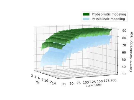
Fig. 10 shows the dependence of the correct classification rate on the number of fuzzy terms for both probability and possibility approaches. Here, the results are averaged on five data sets. We can clearly see that the probability framework (in dark green) gives better results than the possibilistic one (in light blue). We merged the numbers of terms for N and O in one axis using a technique thoroughly described below, in the explanation of fig. 11.

To avoid bias due to the differences in the sizes of the trees, we ran the test setting the entropy and non-specificity gain thresholds so that the number of leaves of the trees are similar in the two approaches : the average number of leaves is close to 500 for a threshold of 0.1 in the probabilistic case, and 0.15 in the possibilistic case.

We can then conclude that the probabilistic approach is better than the possibilistic approach for our problem of material classification from impre-cise chemical data. One reason might be that the possibilistic T-conorm, max, does not take into account the whole distribution which represents the input datum, and only considers a single value. On the contrary, the integral used in the probabilistic model grasps the sense of the whole distribution by computing the average of all the contributions.

nC

2 4 6 8₁₀₁₂₁₄

nO+ 14nN

25 50 75 100 125 150175 200

Correct classification rate

30 40 50 60 70 80 90 Probabilistic modeling Possibilistic modeling

Figure 10: Correct classification rate against number of fuzzy terms for both approaches

Fig. 11 illustrates the grid-based tests we performed with the probabilis-tic framework for numbers of terms varying from 2 to 14 for C, N and O, and set to 5 for the other elements. The graph displays the accuracy as a function of the numbers of terms for C, N and O. In order to represent this dependence in a 3D graph, we merged the N and O numbers of terms on one axis. Every test is represented as a point of coordinates (nC, nO+ 14nN, r),

where nC, nN and nO are the numbers of terms for C, N and O respectively,

and r is the correct classification rate. The points corresponding to a same value of nN are linked into a surface. Multiplying nN by 13 would have been

sufficient to guarantee the injectivity of the representation but we multiplied by 14 to let a gap between two consecutive surfaces for the sake of visibility. We can see that higher numbers of terms for N and O increase the accuracy but that a relatively low number of terms for C is enough to obtain good correct classification rates. The best combination turned out to be 5 terms for C, 14 for N and 12 for O. In the following, we will present further results for the probabilistic framework, with this optimal combination.

4.3 Results analysis

In the probabilistic approach, our treatment of the imprecision of the data does improve the accuracy compared to the same method without taking into account this imprecision, i.e. considering the data as discrete values -the means of -the imprecision distributions. Fig. 12 represents -the difference of correct classification rate with and without imprecision treatment. The gain of the imprecision treatment increases with the degree of imprecision of the data (see the definition in 4.1).

Fig. 13 is a confusion matrix which summarizes the results of the prob-abilistic method on the 26-class drug/explosive problem with the optimal combination of 14 fuzzy terms for carbon, 14 for nitrogen and 13 for oxygen. We can see that the algorithm classes quite correctly both the explosives (seventeen first classes from the top in ordinate) and the drugs (six last classes). The correct classification rate is 88.08%.

We also tested the method with the same parameters on a more complex problem with 38 classes of drugs, explosives and benign materials. The accuracy obtained is a bit lower : 79% of correct classification (see confusion matrix in fig. 14).

5

Conclusion

We presented a workflow for explainable material recognition from chemical compositions, based on linguistic variables learning and fuzzy decision tree induction. We implemented both probabilistic and possibilistic approaches. The probabilistic framework is actually an hybrid probabilistic/fuzzy ap-proach since it takes a Gaussian probability distribution as an input and apply a fuzzy inference process to it. The comparison between the two approaches showed that the probabilistic one provides better results.

The method takes into account the imprecision of the data in both train-ing and evaluation phases. In the probabilistic case, it outperforms the method without imprecision treatment and this gain increases with the de-gree of imprecision of the input data. We obtained correct classification rates up to 85%.

Several refinements may allow us to enhance our method’s accuracy in further work. We might improve the linguistic terms learning using other

nC

2 4 6

8 10 12 _{14 25 50}75100nO+14nN

125150175200

Correct classification rate

50 60 70 80 90 nC₁₄12246810 nO+ 14nN 25 50 75 100 125 150 175 200

Correct classification rate

50 60 70 80 90

Figure 11: Correct classification rate against number of fuzzy terms - two views of the same graph

Figure 12: Gain obtained when taking the imprecision of the data into account 0 5 10 15 20 25 0 5 10 15 20 25 0 2 4 6 8 10

0 5 10 15 20 25 30 35 0 5 10 15 20 25 30 35 0 2 4 6 8 10

Figure 14: Confusion matrix for drugs, explosives and benigns dissimilarities, and taking the samples’ labels into account. We shall also experiment more sophisticated aggregation methods than the mere addition of the results associated to each leaf. Some post-pruning techniques could be used along with the pre-pruning criteria to avoid trees with too many rules. Simpler rules, corresponding to the intern nodes of the tree, might also be useful in the classification.

We will soon be able to evaluate our method on real data sets with high imprecision. Data acquisition on pure elements, chemical products, drug and explosive simulants are being performed. This will be a first step since we will eventually have to address the problem of recognition of mixtures and materials into matrices, that are very frequent in real life container voxels.

Acknowledgment

This project has received funding from the European Union’s Horizon 2020 research and innovation program under grant agreement No 653323. We warmly thank S. Moretto, C. Fontana, F. Pino, A. Sardet, C. Carasco, B. P´erot and V. Picaud for their contributions before our work, for their availability and their expertise.

References

[1] T. Akiyama and H. Inokuchi, “Application of fuzzy decision tree to analyze the attitude of citizens for wellness city development,” in 2016 17th International Symposium on Advanced Intelligent Systems, 2016. [2] M. Aupetit, L. Allano, I. Espagnon, and G. Sanni´e, “Visual analytics

to check marine containers in the eritr@c project,” in Proceedings of International Symposium on visual analytics science and technology, 2010, pp. 3 – 4.

[3] M. Bounhas, H. Prade, M. Serrurier, and K. Mellouli, “A possibilis-tic rule-based classifier,” in IPMU 2012 : Advances on computational intelligence, 2012.

[4] R. L. P. Chang and T. Pavlidis, “Fuzzy decision tree algorithms,” IEEE Transactions on Systems, Man and Cybernetics, vol. 7, no. 1, pp. 28 – 35, 1977.

[5] W. Duch, “Uncertainty of data, fuzzy membership functions, and mul-tilayer perceptrons,” IEEE Transactions on Neural Networks, vol. 16, no. 1, pp. 10 – 16, 2005.

[6] B. J. Frey and D. Dueck, “Clustering by passing messages between data points,” Science, 2007.

[7] M. Higashi and G. J. Klir, “Measures of uncertainty and information based on possibility distributions,” International journal of general sys-tems, 1982.

[8] A. G. Huizing, A. Theil, and F. C. A. Groen, “A comparison of a possibilistic and a probabilistic classifier in a multitarget tracking en-vironment,” in Proccedings of IEEE 1997, 1997.

[9] H. Ishibuchi, T. Nakasima, and T. Morisawa, Fuzzy sets and Systems. Elsevier, 1999, ch. Voting in fuzzy rule-based systems for pattern clas-sification problems, pp. 223–238.

[10] I. Jenhani, N. B. Amor, and Z. Elouedi, “Decision trees as possibilistic classifiers,” International journal of approximate reasoning, 2008. [11] L. Kaufman and P. J. Rousseeuw, Statistical data analysis based on

the L1 norm and related methods. Y. Dodge, 1987, ch. Clustering by

means of medoids, pp. 405–416.

[12] E. Nikolaidis, S. Chen, H. Cudney, R. T. Haftka, and R. Rosca, “Com-parison of probability and possibility for design against catastrophic failure under uncertainty,” Transactions of the ASME, 2004.

[13] C. Olaru and L. Wehenkel, “A complete fuzzy decision tree technique,” Fuzzy sets and systems 138, pp. 221–254, 2003.

[14] Y. Peng and P. A. Flach, “Soft discretization to enhance the continuous decision tree induction,” Integrating Aspects of Data Mining, Decision Support and Meta-Learning, 2001.

[15] S. Tsang, B. Kao, K. Y. Yip, Wai-Shing, and S. D. Lee, “Decision trees for uncertain data,” IEEE Transactions on Knowledge and Data Engineering, 2009.