• Aucun résultat trouvé

The intersection problems of parametric curve and surfaces by means of matrix based implicit representations

N/A
N/A
Protected

Academic year: 2021

Partager "The intersection problems of parametric curve and surfaces by means of matrix based implicit representations"

Copied!
22
0
0

Texte intégral

(1)

HAL Id: hal-00809325

https://hal.inria.fr/hal-00809325v2

Preprint submitted on 17 Apr 2013

HAL is a multi-disciplinary open access

archive for the deposit and dissemination of

sci-entific research documents, whether they are

pub-lished or not. The documents may come from

teaching and research institutions in France or

abroad, or from public or private research centers.

L’archive ouverte pluridisciplinaire HAL, est

destinée au dépôt et à la diffusion de documents

scientifiques de niveau recherche, publiés ou non,

émanant des établissements d’enseignement et de

recherche français ou étrangers, des laboratoires

publics ou privés.

The intersection problems of parametric curve and

surfaces by means of matrix based implicit

representations

Ba Thang Luu

To cite this version:

Ba Thang Luu. The intersection problems of parametric curve and surfaces by means of matrix based

implicit representations. 2013. �hal-00809325v2�

(2)

The intersection problems of parametric curve

and surfaces by means of matrix based implicit

representations

Thang Luu Ba

Abstract In this paper, we introduce and study a new implicit representation of parametric curves and parametric surfaces . We show how these representations which we will call the matrix implied, establish a bridge between geometry and linear algebra, thus opening the possibility of a more robust digital processing. The contribution of this approach is discussed and illustrated on important issues of geometric modeling and Computer Aided Geometric Design (CAGD) : The curve/curve, curve/surface and surface/surface intersection problems, the point-on-curve and inversion problems, the computation of singularities points.

Keyword Geometric modeling, parametric curves and surfaces, intersection, pencils of matrix, singular points.

1 Introduction

Rational algebraic curves and surfaces can be described in some different ways, the most common being parametric and implicit representations. Parametric representa-tions describe the geometric object as the closed image of a rational map and implicit representations describe it as the zero set of a polynomial equation. Both represen-tations have a wide range of applications in Computer Aided Geometric Design and Geometric Modeling. A parametric representation is much easier for drawing a sur-face but more difficult for checking if a point lies on a sursur-face whereas an implicit representation is more difficult for drawing a surface but much easier for checking if a point lies on a surface. Implicit representation of parametric curves and paramet-ric surfaces as a matrix has been addressed many times in literature (for example [MC91, SC95, CGZ00, BCD03]). However, it has always been in order to write an

Thang, Hanoi National University of Education, Department of Mathematics and Informatics, 136 Xuan Thuy, Cau Giay, Hanoi, Vietnam and INRIA, Galaad, 2004 route des Lucioles, 06902 Sophia Antipolis, France; e-mail: thanglb@hnue.edu.vn

(3)

implicit equation as the determinant of a square matrix. The case of planar curves is particularly well known because one always know how to find such a simple square matrix. We can read the article of T. Sederberg and F. Chen [SC95]who introduced this technique to the problems intersection between plane curves for modeling ge-ometric. The case of parametric surfaces is especially much more difficult because the geometry of their parameterizations becomes richer with the inevitable appear-ance of base points (these are points where a parameterization is not well defined). In order to find a square matrix whose determinant is an implicit equation, must be restricted to particular classes of parameterizations [CGZ00, BCD03, AC06], which turns out to be very restrictive in practice.

In this paper, we show how, by releasing the constraint matrix square, we can easily form a implicit representation in the form of a matrix for a parametric sur-face very general. The matrix in question is no longer square, but still allows to characterize the surface: the cancellation a determinant is replaced here by a prop-erty of rank drop. In addition, treatment of intersection problems can be reduced to linear algebra computations digital, allowing the operation of robust tools and per-forming for the approximate calculation, such as the singular value decomposition, calculating eigenvalues and generalized eigenvectors. Note that these implicit rep-resentation matrices can be seen as a bridge between the parametric reprep-resentation of curve, surface and its implicit representation.

This article covers a series of works [BJ03, BC05, BCJ09, BCAS10, BD07, BB10], which led to the notion of implicit representation matrix of a parametric curve or a parametric surface, together with the development of applications for in-tersection problems in geometric modeling [BBM09, BB10, BB12]. Its content is part of authour’s PhD thesis [Ba11].

2 Matrix based implicit representations of parametric surfaces

2.1 Construction of matrix representations

Given a parametric algebraic surface, we briefly recall from [BJ03, BC05] how to build a matrix that represents this surface in a sense that we will make explicit. So suppose given a parameterization

P2R→ Pφ 3R

(s : t : u) 7→ ( f1: f2: f3: f4)(s,t, u)

of a surface S such that gcd( f1, . . . , f4) ∈ R \ {0}. Set d := deg( fi) ≥ 1, i = 1, 2, 3, 4

and denote by x, y, z, w the homogeneous coordinates of the projective space P3 R.

Notice that s,t, u are the homogeneous parameters of the surface S and that an affine parameterization of S can be obtained by ”inverting” one of these parameters; for instance, setting s= s/u and t= t/u we get the following affine parameterization

(4)

of S: R2 φ→ R3 (s,t′) 7→ f 1(s,t′, 1) f4(s,t′, 1) , f2(s,t, 1) f4(s,t′, 1) , f3(s,t, 1) f4(s,t′, 1) 

The implicit equation of S is a homogeneous polynomial S(x, y, z, w) ∈ R[x, y, z, w] of smallest degree such that S( f1, f2, f3, f4) = 0 (observe that it is defined up to

multiplication by a nonzero element in R). It is well known that the quantity deg(S) deg(φ ) is equal to d2 minus the number of common roots of f

1, f2, f3, f4

in P2R, that are called base points of the parameterizationφ , counted with suitable

multiplicities (see for instance [BJ03, Theorem 2.5] for more details). The notation deg(S) stands for the degree of the surface S that is nothing but the degree of the implicit equation of S.

The notation deg(φ ) stands for the degree of the parameterization φ (co-restricted to S) that, roughly speaking, measures the number of times the surface S is drawn by the parameterizationφ . More precisely, deg(φ ) is equal to the number of pre-images of a general point on S by the parameterizationφ .

For all non negative integerν, we build a matrix M(φ )νas follows. Consider the

set L(φ )ν of polynomials of the form

a1(s,t, u)x + a2(s,t, u)y + a3(s,t, u)z + a4(s,t, u)w

such that

• ai(s,t, u) ∈ R[s,t, u] is homogeneous of degree ν for all i = 1, . . . , 4,

• ∑4

i=1ai(s,t, u) fi(s,t, u) ≡ 0 in R[s,t, u].

The set L(φ )ν has a natural structure of R-vector space of finite dimension

be-cause each polynomial ai(s,t, u) is homogeneous of degree ν and that the set of

homogeneous polynomials of degreeν in the variables s,t, u is a R-vector space of dimension ν+22 with canonical basis the set of monomials{sν, sν−1t, · · · , uν}. So, denote by L(1), . . . , L(nν) a basis of the R-vector space L(φ )ν; it can be computed by solving a single linear system whose indeterminates are the coefficients of the polynomials ai(s,t, u), i = 1, 2, 3, 4. The matrix M(φ )ν is then by definition the

ma-trix of coefficients of L(1), . . . , L(nν)as homogeneous polynomials of degreeν in the variables s,t, u. In other words, we have the equality of matrices:


sν sν−1t· · · uνM(φ )ν =


L(1)L(2) · · · L(nν).

Notice that we have chosen for simplicity the monomial basis for the R-vector space of homogeneous polynomials of degreeν in s,t,u. However, any other choice, for instance the Bernstein basis, can be made without affecting the result.

For all integerν≥ 2d − 2, the matrix M(φ )νis said to be a representation matrix ofφ because it satisfies the following properties under the assumption that the base points ofφ , if any, form locally a complete intersection, which means that at each

(5)

base point, the ideal of polynomials( f1, f2, f3, f4) can be generated by two equations

(see [BJ03, Definition 4.8] for more details):

• The entries of M(φ )νare linear forms in R[x, y, z, w].

• The matrix M(φ )ν has ν+22


rows (which is nothing but the dimension of the R-vector space of homogeneous polynomials of degreeν in three variables, here

s,t, u) and possesses at least as much columns as rows. • The rank of M(φ )ν is ν+22 .

• When specializing M(φ )νat a given point P∈ P3R, its rank drops if and only if P

belongs to S.

• The greatest common divisor of the ν+22 -minors of M(φ )νis equal to the implicit

equation of S raised to the power deg(φ ).

From a computational point of view, the matrix M(φ )ν with the smallest possible

value ofν has to be chosen. It is rarely a square matrix. Also, notice that the last property given above is never used for computations; our aim is to keep the matrix M(φ )νas an implicit representation of S in place of its implicit equation.

There are many results that lead to enlarge the above family of matrices and to make it available in other contexts. Since a detailed overview of these results is not the main purpose of this paper, we just recall them shortly with appropriate references to the literature:

• The hypothesis on the base points of φ can be relaxed. If the base points are locally almost complete intersection, meaning that they are locally given by three (and not two) equations, then the above family of matrices can still be constructed and provide a matrix representation of the surface S plus a certain product of hyperplanes that can be described from the parameterizationφ . In addition, the bound 2d− 2 for the integer ν can be decreased. See [BC05, BJ03].

• In our setting, φ parameterizes what is called a triangular Bezier patch. It turns out that a similar family of matrices M(φ )ν can be built for parameterizations

of tensor product surfaces, and even for any parameterization whose parame-ter space is a projective toric variety (triangular and tensor product surfaces are particular cases of parameterizations whose parameter space is a projective toric variety). We refer the interested reader to [BD07, BDD09].

• To build the matrices M(φ )νwe used what is called moving planes, that is to say

syzygies of the parameterizationφ . It is actually possible to build another fam-ily of matrices by taking into account moving quadrics, i.e. syzygies associated to the square of the ideal generated by the parameterization ofφ . In this way, we get a family containing smaller matrices whose entries are either linear or quadratic forms in R[x, y, z, w]. In some sense, they generalize the matrices given in [CGZ00] and [BCD03]. See [BCAS10].

Example 1.The Steiner surface S of degree 2 parameterized by φ1: P2→ P3:(s : t : u) 7→ (s2+ t2+ u2: tu : st : su)

(6)

M(x, y, z, w) :=         −x 0 −y 0 −y y 0 z 0 y −y 0 w 0 −x −y 0 0 0 0 w 0 0 0 z 0 −x w 0 0 −y 0 z 0 −y y 0 w 0 0 0 z 0 0 y w 0 0 0 z 0 0 0 y         .

Example 2.Let S be the rational surface of degree 3 which is parametrized by φ : P2→ P3:(s : t : u) 7→ ( f1: f2: f3: f4)

where

f1= s3+ t2u, f2= s2t+ t2u, f3= s3+ t3, f4= s2u+ t2u.

Then, a matrix representation of S is         0 0 0 w− y 0 0 z− x w 0 0 x w− y 0 0 x− y − z 0 0 −z 0 w− y 0 0 w 0 0 x 0 −y 0 x− y − z w 0 −z x y+ z − x 0 0 x− y − z 0 0 −z 0        

2.2 Points on surface and inversion problem

Suppose given a parameterizationφ of a parametric surface S and a point P in P3.

Denote by M(φ )ν a matrix representation ofφ for some integer ν ≥ ν0. Since its

entries are linear forms in the variables s,t, u, one can evaluate M(φ )νat P and get a

matrix with coefficients in the ground field R. Then, we have that rank(M(φ )ν(P)) < ν + 1 if and only if P ∈ S.

This property answers the point-on curve problem.

If rank M(φ )ν(P) = rank M(φ )ν− 1 = ν then P has a unique pre-image (s0: t0: u0)

by φ and moreover, this pre-image can be recovered from the computation of a generator, say WP= (w0, . . . , wν) ∈ Rν+1, of the kernel of the transpose of M(φ )ν(P).

Indeed, if b0(s,t, u), . . . , bν(s,t, u) is the basis of R[s,t, u]ν that has been chosen to

build M(φ )ν, then there existsλ∈ R \ {0} such that

WP= λ (b0(s0,t0, u0), . . . , bν(s0,t0, u0)) .

For instance, suppose that bi(s,t, u) = sitjuν−i− j, 0≤ i, j ≤ ν, i + j ≤ ν (the usual

(7)

Obviously, the inversion problems have been tranfered to compute kernel of transposed matrix of M(φ )ν(P) that exits numerical effective algorithms such as

SVD (Singular Value Decomposition).

We also point out that the points P∈ S such that rank M(φ )ν(P) = rank M(φ )ν− 1= ν are precisely the regular points on S, that is to say that all the points that do not verify this property are singular points on S.

3 Curve/surface Intersection

Suppose given a parametric surface S represented by a homogeneous and irreducible implicit equation S(x, y, z, w) = 0 in P3

Rand a rational space curve C represented by

a parameterization

Ψ : P1R→ P3R:(s : t) 7→ (x(s,t) : y(s,t) : z(s,t) : w(s,t))

where x(s,t), y(s,t), z(s,t), w(s,t) are homogeneous polynomials of the same degree and without common factor in R[s,t].

A standard problem in non linear computational geometry is to determine the set C∩ S ⊂ P3R, especially when it is finite. One way to proceed, is to compute the roots of the homogeneous polynomial

S(x(s,t), y(s,t), z(s,t), w(s,t)) (1) because they are in correspondence with C∩ S through the regular map Ψ . Observe that (1) is identically zero if and only if C∩ S is infinite, equivalently C ⊂ S (for C is irreducible).

Assume that M(x, y, z, w) is a matrix representation of the surface S, meaning a representation of the polynomial S(x, y, z, w). By replacing the variables x, y, z, w by the homogeneous polynomials x(s,t), y(s,t), z(s,t), w(s,t) respectively, we get the matrix

M(s,t) = M(x(s,t), y(s,t), z(s,t), w(s,t))

therefore, we have the following easy property: for all point(s0: t0) ∈ P1Rthe rank

of the matrix M(s0,t0) drops if and only if the point (x(s0,t0) : y(s0,t0) : z(s0,t0) : w(s0,t0)) belongs to the intersection locus C ∩ S.

It follows that points in C∩ S associated to points (s : t) such that s 6= 0, are in correspondence with the set of values t∈ R such that M(1,t) drops of rank strictly less than its row and column dimensions i.e. the set of generalized eigenvalues of

M(1,t). Now, we present a tenichque of linear algebra which permet us to obtain the regular part of the pencil matrices.

(8)

3.1 Linearization of a polynomial matrix

We begin with some notation. Let A and B be two matrices of size m× n with coefficients in R. We will call a generalized eigenvalue of A and B a value in the set

λ(A, B) := {t ∈ K : rank(A − tB) < min{m, n}}.

In the case m= n, the matrices A and B have n generalized eigenvalues if and only if rank(B) = n. If rank(B) < n, then λ (A, B) can be finite, empty or infinite. Moreover, if B is invertible then λ(A, B) = λ (AB−1, I) = λ (AB−1), which is the ordinary spectrum of AB−1.

Suppose given an m× n-matrix M(t) = (ai, j(t)) with polynomial entries ai, j(t) ∈

R[t]. It can be equivalently written as a polynomial in t with coefficients m × n-matrices with entries in R: if d= maxi, j{deg(ai, j(t))} then

M(t) = Mdtd+ Md−1td−1+ . . . + M0

where Mi∈ Rm×n.

The generalized companion matrices A, B of the matrix M(t) are the matrices with coefficients in R of size((d − 1)m + n) × dm that are given by

A=        0 Im . . . 0 0 0 Im . . . 0 .. . ... ... ... ... 0 0 . . . Im M0t M1t . . . Mt d−1        B=        Im 0 . . . 0 0 Im 0 . . . 0 .. . ... ... ... ... 0 0 . . . Im 0 0 0 . . . −Mt d       

where Im stands for the identity matrix of size m and Mit stands for the transpose

of the matrix Mi. These companion matrices allows to linearize the polynomial

ma-trix M(t) in the sense that there exists two unimodular matrices E(t) et F(t) with coefficients in C[t] and of size dm and (d − 1)m + n respectively, such that

E(t) (A − tB) F(t) = t M(t) 0 0 Im(d−1)  . (2) Then, we have

(9)

We recall t such that rank(A − tB) drops the generalized eigenvalues of the pencil matrices A− tB. So. we transformed the computation of generalized eigenvalues of the matrix polynomial M(t) into the computation of generalized eigenvalues of a pencil of matrices A− tB. If the matrices A, B were two square matrices, then we could easily compute their generalized eigenvalues by the QZ-algorithm [GVL96]. Therefore, our next task is to reduce the pencil A−tB into a square pencil that keeps the information we are interested in.

3.2 Extracting the regular part of a non square pencil of matrices

For any couple constant matrices A, B of size p× q, there exist constant invertible matrices P and Q such that the pencil P(A − tB)Q is of the block-diagonal form

diag{Li1, ..., Lis, L t j1, ..., L t ju, Ωk1, ..., Ωkv, A− tB}

where A, Bare square matrices and Bis invertible. The dimension i

1, ..., is, j1, ..., ju, k1, .., kv

and the determinant of A−tB(up to a scalar) are independent of the representation.

Where Lk(t), Ωk(t) are the two matrices of size k × (k + 1) and k × k respectively,

defined by Lk(t) =        1 t 0 . . . 0 0 1 t . . . 0 .. . ... ... ... ... 0. . . 1 t 0 0 0 . . . 1 t        , Ωk(t) =        1 t 0 . . . 0 0 1 t . . . 0 .. . ... ... ... ... 0. . . 1 t 0 0 . . . 0 1        .

One called this form the Kronecker canonical form of a pencil of matrices (see for instance [Gan66, p. 31-34]).

It is interesting to notice that the above decomposition can be computed within

O(p2q) arithmetic operations. We refer the reader to [BVD88] for a proof, as well

as for an analysis of the stability of this decomposition.

Following the ideas developed in [BVD88] and the reduction methods exploited in [Mou05], we now describe an algorithm that allows to remove the Kronecker blocks Lk, LtkandΩkof the pencil of matrices A− tB in order to extract the regular

(10)

We start with a pencil A− tB where A, B are constant matrices of size p × q with coefficients in a field R. Setρ = rank B. In the following algorithm, all computa-tional steps are easily realized via the classical LU-decomposition.

• Transform B into its column echelon form; that amounts to determine unitary matrices P0and Q0such that

B1= P0BQ0= [B1,1 |{z} ρ | 0 |{z} q−ρ ]

where B1,1is an echelon matrix. Then, compute A1= P0AQ0= [A1,2 |{z} ρ | A1,2 |{z} q−ρ ]

• Transform A1,2into its row echelon form; that amounts to determine unitary

ma-trices P1and Q1such that

P1A1,2Q1=


A1,2

0 

where A1,2has full row rank while keeping B1,1in echelon form.

Then we obtain a new pencil of matrices, namely A2− tB2.

• Starting from j = 2, repeat the above steps 1 and 2 for the pencil Aj− tBjuntil

the pj× qjmatrix Bjhas full column rank, that is to say until rank Bj= qj.

• If Bj is not a square matrix, then we repeat the above procedure with the

trans-posed pencil Atj− tBt j.

At last, we obtain the regular pencil A−tBwhere A, B′are two square matrices and B′is invertible. Moreover, we have the

rank(A − tB) drops ⇔ rank(A′− tB′) drops.

We are now ready to state our algorithm for solving the curve/surface intersection problem:

Algorithm 1: Matrix intersection algorithm

Input: A matrix representation of a surface S and a parametrization of a rational space curve C .

Output: The intersection points of S and C .

1. Compute the matrix representation M(t).

2. Compute the generalized companion matrices A and B of M(t). 3. Compute the companion regular matrices Aand B.

4. Compute the eigenvalues of(A, B).

5. For each eigenvalue t0, the point P(x(t0) : y(t0) : z(t0) : w(t0)) is one of the intersection

(11)

Remark that this algorithm returns all the points in C ∩ S except possibly the pointφ(1 : 0). This latter point can be treated independently.

Example 3.Let S be the sphere that we suppose given as the image of the parametriza-tion

φ : P2→ P3:(s : t : u) 7→ ( f1: f2: f3: f4)

where

f1= s2+ t2+ u2, f2= 2su, f3= 2st, f4= s2− t2− u2

Let C be the twisted cubic which is parametrized by

x(t) = 1, y(t) = t, z(t) = t2, w(t) = t3.

The computation of a matrix representation of the sphere S gives   −y 0 z x+ w 0 −y −x + w −z z x+ w y 0  .

Now, a point P belongs to the intersection of S and C if and only if P= (1 : t :

t2: t3) and t is one of the generalized eigenvalues of the matrix M(t) =   −t 0 t2 1+ t3 0 −t −1 + t3 −t2 t2 1+ t3 t 0  . As before, we easily compute the eigenvalues and find:

t1= 0.7373527056,t2= −0.7373527056,

t3= 0.5405361044 + 1.031515287i,t4= −0.5405361044 − 1.031515287i, t5= 0.5405361044 − 1.031515287i,t6= −0.5405361044 + 1.031515287i.

All these eigenvalues have multiplicity 1. They all correspond to one intersection point between S and C which has multiplicity 1. By Bezout Theorem, we find here all the intersection points between these two algebraic varieties (all of them are at finite distance).

4 Surface/surface intersection

Computing the intersection between two parametric algebraic surfaces is a funda-mental task in Computer Aided Geometric Design. Several methods and approaches have been developed for that purpose. Some of them are based on the use of matrix representations of the objects because they allow to transform geometric operations on the intersection curve into matrix operations. This approach seems to have been

(12)

Fig. 1: Intersection of the sphere and the twisted cubic, the axis Oz

first introduced by J. Canny and D. Manocha in their paper [MC91]. Roughly speak-ing, it consists in representing the implicit equation of one of the two surfaces as the determinant of a certain matrix, necessarily square. Then, instead of using this im-plicit equation, the matrix itself is used as a representation of this first parametric surface and then a matrix representation of the intersection curve is easily obtained by substituting the implicit variables with the parameterization of the second face. In this section, we extend the approach of Canny and Manocha about sur-face/surface intersection for a significantly larger class of parameterizations which have been introduce in Section 2.

Suppose given two distinct parametric surfaces S1and S2. A standard problem in

non linear computational geometry is to determine the set S1∩ S2which is a curve

in P3C. As we explained above, one can build a representation matrix of S1that we

will denote by M(x, y, z, w). Let

Ψ : P2C→ P3C:(s : t : u) 7→ (a(s,t, u) : b(s,t, u) : c(s,t, u) : d(s,t, u))

be a parameterization of S2where a(s,t, u), b(s,t, u), c(s,t, u), d(s,t, u) are

homoge-neous polynomials of the same degree and without common factor in C[s,t, u]. By substituting in the matrix M(x, y, z, w) the variables x, y, z, w by the homogeneous polynomials a(s,t, u), b(s,t, u), c(s,t, u), d(s,t, u) respectively, we get the matrix

M(s,t, u) := M(Ψ (s : t : u)) = M(a(s,t, u), b(s,t, u), c(s,t, u), d(s,t, u)). From the properties of the representation matrix M(x, y, z, w), we known that M(s,t, u) has maximal rank ρ (ρ is the number of rows of M). Moreover, for all point (s0: t0: u0) ∈ P2Rwe have

(13)

rank(M(s0,t0, u0)) < ρ if and only if

(

Ψ(s0: t0: u0) ∈ S1∩ S2or

(s0: t0: u0) is a base point of Ψ .

(3) The equivalence (3) shows that the spectrum of the matrix M(s,t, u), that is to say the set


(s0: t0: u0) ∈ P2Rsuch that rank M(s0,t0, u0) < ρ

,

yields the intersection locus S1∩ S2plus the base points of the parameterizationΨ

of S2.

In [BB12] we proved that the spectrum of the matrix M(s,t, u) is an algebraic curve in P2R, that is to say is equal to the zero locus of a homogeneous polynomial

in C[s,t, u]. In particular, there is no isolated points in the spectrum of M(s,t, u). As a consequence if we use matrix representations to deal with the surface/surface intersection problem, we will end up at some point with a pencil of bivariate and non-square matrices that represents the intersection curve (after dehomogenization). Therefore, in order to be able to handle this intersection curve, for instance to de-termine its exact topology, it is necessary to extract a pencil of bivariate and square matrices that yields a matrix representation of the intersection curve as a matrix de-terminant. For that purpose, we develop an algorithm (called∆W -Decomposition) based on the remarkable work of V. N. Kublanovskaya [KK96, Kub99].

We build two companion matrices A(t) and B(t) which allows to linearize the polynomial matrix M(s,t, 1) such that the spectrum of the matrix M(s,t, 1) coincides the spectrum of the matrix A(t) − sB(t). Then, we provide an algorithm that extracts a square matrix whose determinant represents the intersection locus curve S1∩S2. A

pencil of polynomial matrices A(t) − sB(t) is equivalent to a pencil of the following

form M1,1(s,t) 0 0 M2,1(s,t) M2,2(s,t) 0 M3,1(s,t) M3,2(s,t) M3,3(s,t)  

where the pencil M2,2(s,t) is a regular pencil that corresponds to the intersection

locus curve S1∩ S2.

Now, we get the following algorithm (for more details see [BB12]): Algorithm 2: Matrix representation of an intersection curve

Input: Two parametric algebraic surfaces S1and S2such that the parameterization of S1has

local complete intersection base points.

Output: The intersection curve S1∩ S2represented as a matrix determinant.

1. Compute a matrix representation of S1, say M(x, y, z, w).

2. Substitute x, y, z, w by the parameterization of S2in the matrix M to get a matrix M(s,t)

(set u= 1).

3. Compute the generalized companion matrices A(s) and B(s) associated to M(s,t) .

(14)

In comparison with [MC91], our algorithm returns a result of the same type: a determinant matrix representation of the intersection curve, but the class of pa-rameterizations of surfaces for which step 1 can be performed is here dramatically extended. We present an illustrative example.

Example 4.We start with the Steiner surface S1parameterized by

φ1: P2→ P3:(s : t : u) 7→ (s2+ t2+ u2: tu : st : su)

which admits the matrix representation

M(x, y, z, w) :=         −x 0 −y 0 −y y 0 z 0 y −y 0 w 0 −x −y 0 0 0 0 w 0 0 0 z 0 −x w 0 0 −y 0 z 0 −y y 0 w 0 0 0 z 0 0 y w 0 0 0 z 0 0 0 y         .

We want to study the intersection between S1and the cubic surface S2parameterized

by

φ2: P2→ P3:(s : t : u) 7→ (s3+ t3: stu : su2+ tu2: u3).

As in the previous example, to determine the intersection between S1and S2we will

compute the spectrum of the polynomial matrix

M(s,t, u) =        

−s3− t3 0 −stu 0 −stu stu 0 su2+ tu2 0 stu −stu 0 u3 0 −s3− t3 −stu 0 0

0 0 u3 0 0 0 su2+ tu2 0 −s3− t3 u3 0 0 −stu 0 su2+ tu2 0 −stu stu

0 u3 0 0 0 su2+ tu2 0 0 stu u3 0 0 0 su2+ tu2 0 0 0 stu         .

By dehomogenizing with respect to the variable u, we consider

M(s,t) =         −s3− t3 0 −st 0 −st st 0 s+ t 0 st −st 0 1 0 −s3− t3 −st 0 0 0 0 1 0 0 0 s+ t 0 −s3− t3 1 0 0 −st 0 s+ t 0 −st st 0 1 0 0 0 s+ t 0 0 st 1 0 0 0 s+ t 0 0 0 st         .

Writing M(s,t) under the form M(s,t) = M3t3+ M2t2+ M1t+ M0, we obtain the

generalized companion matrices of M(s,t):

A(s) =   0 I6 0 0 0 I6 M0t Mt1Mt2  , B(s) =   I6 0 0 0 I6 0 0 0 −Mt 3  .

(15)

Applying the algorithm that extracts a square matrix for the pencil At(s) − tBt(s),

we obtain its regular part M1(s,t) = A1(s) − tB1(s) where

A1(s) =                   s0 1 1 0 0 0 0 0 0 0 0 0 0 s 0 0 0 0 0 0 0 0 0 s0 0 0 0 0 0 0 0 0 0 0 1 0 0 0 0 0 1 0 0 0 0 0 1 0 0 0 0 0 0 1 0 0 0 0 0 0 0 0 1 0 0 0 0 0 0 0 0 0 0 0 0 1 0 0 0 0 0 0 s0 0 0 0 0 0 0 1 0 0 0 0 1 0 0 0 0 0 0 0 0 0 0 0 0 0 0 0 0 0 0 0 1 0 0 0 0 0 0 0 0 0 0 0 0 1 0 0 0 0 0 0 0 0 0 0 0 0 1                   , B1(s) =                   −s21 0 0 0 −s 0 0 s 0 0 0 s3 s s41 0 0 s30 s20 0 0 0 0 s 0−1 0 1 0 0 0 0 0 0 0 0 0 0 0 0 0 0 1 0 0 0 0 0 0 0 0 0 0 0 0 1 0 0 0 0 0 0 0 0 0 0 0 0 1 1 0 0 0 1 0 0 0 0 0 0 0 0 0 0 0−1 0 0 1 0 0 0 0 s 0 0 0 0 1 0 0 0 0 0 0 0 0 0 0 0 0 0 0 0 0 0 0 0 0 0 0 0 0 0 0 0 0 0 0 0 0 0 0 0 0 0 0 0 0 0 0                   .

Its yields a plane curve of degree 6 whose implicit equation is det(M1(s,t)) = t2+

2st+ s2t2+ 2s3t3− st5+ s2− ts5. This plane curve parameterizes S

1∩ S2through

the regular mapφ2.

5 Matrix -based implicit representations of parametric curves in

space

Let f0, f1, f2, f3be homogeneous polynomials in R[s,t] of the same degree d ≥ 1

such that their greatest common divisor (GCD) is a non-zero constant in R. Consider the regular map

P1R→ Pφ 3R

(s : t) 7→ ( f0: f1: f2: f3)(s,t).

The image ofφ is an algebraic curve C in P3

Rwhich is called a rational curve.

5.1 Construction of representation matrix

Consider the set of syzygies of f := ( f0, f1, f2, f3), that is to say the set

Syz(f) = ( (g0(s,t), . . . , g3(s,t)) : 3

i=0 gi(s,t) fi(s,t) = 0 ) ⊂ 3 M i=0 R[s,t] From a classical structure theorem of commutative algebra called the Hilbert-Burch Theorem (see for instance [Eis,§20.4]), Syz(f) is known to be a free and graded R[s,t]-module of rank 3. Moreover, there exists non-negative integers µ1, µ2, µ3and 3 vectors of polynomials

(16)

such that

• for all i ∈ {1, 2, 3}, j ∈ {0, 1, 2, 3}, ui, j(s,t) is a homogeneous polynomial in

R[s,t] of degree µi≥ 0,

• the 3 vectors in (4) form a R[s,t]-basis of Syz(f), • µ1+ µ2+ µ3= d,

• For all j ∈ {0, . . . , 3}, the determinant of the matrix obtained by deleting the column(ui, j)i=1,2,3from the matrix

M(s,t) :=   u1,0(s,t) u1,1(s,t) u1,2(s,t) u1,3(s,t) u2,0(s,t) u2,1(s,t) u2,2(s,t) u2,3(s,t) u3,0(s,t) u3,1(s,t) u3,2(s,t) u3,3(s,t)   (5) is equal to(−1)jc f j(s,t) ∈ R[s,t] where c ∈ R \ {0}.

A collection of vectors as in (4) that satisfy the above properties is called a µ-basis of the parameterizationφ . It is important to notice that a µ-basis is far from being unique, but the collection of integers(µ1, µ2, µ3) is unique if we order it.

Therefore, in the sequel we will always assume that a µ-basis is ordered so that 0≤ µ1≤ µ2≤ µ3.

For all integer i= 1, 2, 3 and all integer ν ∈ N, consider the matrix Sylvν(ui) that

satisfies to the identity  sν sν−1t · · · stν−1tν× Sylvν(ui) =  sν−µiu isν−µi−1tui · · · stν−µi−1uitν−µiui  . It is a(ν + 1) × (ν − µi+ 1)-matrix which usually appears as a building block in

well known Sylvester matrices. It follows that the matrix Sylvν(u1, u2, u3) =

Sylvν(u1) Sylvν(u2) Sylvν(u3)

 .

It hasν+1 rows and 3(ν +1)−d columns. Its entries are linear forms in R[x0, . . . , x3];

in particular, it can be evaluated at any point(x0:· · · : x3) ∈ P3Rand yields a matrix

with coefficients in R.

In [BB10], we proved that for allν≥ µ3+ µ2−1 the matrix M(φ )ν:= Sylvν(u1, u2, u3)

is a matrix-based representation of the curve C i.e

(i) M(φ )νis generically full rank, that is to say generically of rankν+ 1,

(ii)the rank of M(φ )ν drops exactly on the curve C .

Of course, in practice the most useful matrix is the smallest one, that is to say M(φ )µ3+µ2−1.

Example 5.Let C be the rational space curve parameterized by P1R→ Pφ 3R

(17)

Aµ-basis of C is given by

p= −tx + sy

q= −ty + sz,

r= −t2z+ s2w.

We haveµ1= µ2= 1, µ3= 2 and hence µ3+ µ2− 1 = 2. Therefore, we obtain the

following representation matrix ofφ : M(φ )2=   y 0 z 0 w −x y −y z 0 0 −x 0 −y −z  .

5.2 Points on curves and inversion problems

Suppose given a parameterizationφ of a rational curve C and a point P in P3. Denote

by M(φ )ν a matrix representation ofφ for some integer ν ≥ µ3+ µ2− 1. Since its

entries are linear forms in the variables x0, x1, x2, x3, one can evaluate M(φ )νat P and

get a matrix with coefficients in the ground field R. Then, we have that rank(M(φ )ν(P)) < ν + 1 if and only if P ∈ C .

This property answers the point-on curve problem.

If rank M(φ )ν(P) = rank M(φ )ν− 1 = ν then P has a unique pre-image (s0: t0)

by φ and moreover, this pre-image can be recovered from the computation of a generator, say WP= (w0, . . . , wν) ∈ Rν+1, of the kernel of the transpose of M(φ )ν(P).

Indeed, if b0(s,t), . . . , bν(s,t) is the basis of Cνthat has been chosen to build M(φ )ν,

then there existsλ∈ R \ {0} such that

WP= λ (b0(s0,t0), . . . , bν(s0,t0)) .

For instance, suppose that bi(s,t) = sitν−i, i= 0, . . . , ν (the usual monomial basis),

then(s0: t0) = (w1: w0) if w06= 0, otherwise (s0: t0) = (1 : 0).

We point out that the points P∈ C such that rank M(φ )ν(P) = rank M(φ )ν− 1 = ν are precisely the regular points on C , that is to say that all the points that do not verify this property are singular points on C . We will come back again on this property and on the treatment of the singular points on C in the next section.

(18)

f0(s,t) = 3s4t2− 9s3t3− 3s2t4+ 12st5+ 6t6, f1(s,t) = −3s6+ 18s5t− 27s4t2− 12s3t3+ 33s2t4+ 6st5− 6t6, f2(s,t) = s6− 6s5t+ 13s4t2− 16s3t3+ 9s2t4+ 14st5− 6t6, f3(s,t) = −2s4t2+ 8s3t3− 14s2t4+ 20st5− 6t6. Aµ-basis for C is p= (s2− 3st + t2)x + t2y q= (s2− st + 3t2)y + (3s2− 3st − 3t2)z, r= 2t2z+ (s2− 2st − 2t2)w.

From deg(p) = deg(q) = deg(r) = 2, we have µ3+ µ2− 1 = 3 and hence a matrix

representation of C is given by M(φ )3=     x+ y 0 3y− 3z 0 2z− 2w 0 −3x x + y −y − 3z 3y − 3z −2w 2z − 2w x −3x y + 3z −y − 3z w −2w 0 x 0 y+ 3z 0 w    . Let P= (1 : 1 : 1 : 1) ∈ P3

. Evaluating M(φ )3at P we find that

M(φ )3=     2 0 0 0 0 0 −3 2 −4 0 −2 0 1 −3 4 −4 1 −2 0 1 0 4 0 1     is of rank 4 so that P does not lie on C .

If one evaluates the matrix M(φ )3at the point P= (9 : 9 : 9 : 6) ∈ P3we obtain

the matrix M(φ )3(P) =     18 0 0 0 6 0 −27 18 −36 0 −12 6 9 −27 36 −36 6 −12 0 9 0 36 0 6    .

which has rank 3. Therefore, P is a smooth point on the curve C . Moreover, the computation of the kernel of the transpose of M(φ )3(P) returns the vector (1, 1, 1, 1)

. Thus, we deduce that P= φ (1 : 1).

5.3 Rank of a representation matrix at a singular point

Let P be a point on C . There exists at least one point(s1: t1) ∈ P1such that P=

φ(s1: t1). Now, let H be a plane in P3passing through P, not containing C and

denote by H(x, y, z, w) an equation (a linear form in R[x, y, z, w]) of H . We have the following degree d homogeneous polynomial in R[s,t]

(19)

H( f0(s,t), f1(s,t), f2(s,t), f3(s,t)) = d

i=1

(tis− sit) (6)

where the points(si: ti) ∈ P1, i= 1, . . . , d are not necessarily distinct. We define

the intersection multiplicity of C with H at the point P, denoted iP(C , H ), as the

number of points(si: ti)i=1,...,dsuch thatφ(si: ti) = P.

The multiplicity mP(C ) of the point P on C is defined as the minimum of the

intersection multiplicity iP(C , H ) where H runs over all the hyperplanes not

con-taining C and passing through the point P∈ C , minimum which is reached with a sufficiently generic such H .

Suppose given a representation matrix M(φ )νof the curve C which is built from

the µ-basis p, q, r of degree µ1≤ µ2≤ µ3 correspondence. Its entries are linear

forms in R[x, y, z, w] so that it makes sense to evaluate M(φ )νat a point in P3to get a matrix M(φ )ν(P) with entries in R. In [BB10], we prove the property: Given a point Pin P3, for all integerν≥ µ2+ µ3− 1 we have

rank M(φ )ν(P) = ν + 1 − mP(C ),

or equivalently corank M(φ )ν(P) = mP(C ).

This result provides a stratification of the points in P3with respect to the curve C . Indeed, we have that

• if P is such that rank M(φ )ν(P) = ν + 1 then P 6∈ C ,

• if P is such that rank M(φ )ν(P) = ν then P is a regular point (i.e. of multiplicity

1) on C ,

• if P is such that rank M(φ )ν(P) = ν − 1 then P is singular point of multiplicity 2 on C ,

• and so on.

Moreover, an immediate consequence is that if P is a singular point on C then necessarily

2≤ mP(C ) ≤ µ2 or mP(C ) = µ3. (7)

One can read more details in [BB10] for computational singularities aspects of C .

5.4 Curve/curve intersection

Suppose given two rational curves, say C1parameterized by

P1 φ−→ P1 3:(s : t) 7→ ( f0:· · · : f3)(s,t) (8) and C2parameterized by the regular map

(20)

Let M(φ1)ν be a representation matrix of C1for a suitable integerν. The

substitu-tion in M(φ1)ν of the variables x, y, z, w by the homogeneous parameterization of C2

yields the matrix

M(φ1)ν(s,t) := M(φ1)ν(g0(s,t), . . . , g3(s,t))

As a consequence of the properties of a representation matrix, we have the following property: Let(s0: t0) ∈ P1, then rank M(φ1)ν(s0,t0) < ν + 1 if and only if the point

φ2(s0,t0) belongs to the intersection locus C1∩ C2.

The set C1∩ C2is in correspondence with the points of P1where the rank of

M(φ1)ν(s,t) drops. By setting t = 1, the determination of the values of s such that

the rank of M(φ1)ν(s, 1) can be treated at the level of matrices (that is to say without

any symbolic computation and in particular without any determinant computations) by using linearization technics and generalized eigenvalues computations. We repeat the algorithm which is presented in Section 3.

Algorithm 3: Intersection of two parametric curves

Input: Two parametric curves C1and C2given by (8) and (9).

Output: The intersection points of C1and C2.

1. Compute the matrix representation M(φ )ν(φ1) of C1for a suitableν. 2. Compute the generalized companion matrices A and B of M(φ )ν(φ1). 3. Compute the companion regular matrices Aand B.

4. Compute the eigenvalues of(A, B).

5. For each eigenvalue t0,φ2(t0: 1) is an intersection point.

Remark that this algorithm returns all the points in C1∩ C2except possibly the

pointφ(1 : 0). This latter point can be treated independently.

6 Conclusion

This paper presents a new implicit representation concept of a parametric curve or a parametric surface. This representation is a matrix whose entries are linear forms in the coordinates of R3. This matrix representation characterizes a curve or a

sur-face by a drop rank property. It is easily to calculate, in addition a useful tool for solving intersection problems. Moreover, its main interest is particularly to trans-form intersection problems into numerical linear algebra problems for which we have powerful and robust algorithms to solve such as singular value decomposition, calculating generalized eigenvalues or eigenvectors. Thus, in the context more par-ticularly ray tracing on a surface set, this new approach could improve the robustness of the existing methods in particular situations.

All algorithms that we proposed above have been implemented in the software Maplethat the corresponding files are available at http://cgi.di.uoa.gr/ ˜thanglb/

(21)

Acknowledgements. An part of this work has been completed while the au-thor worked at Department of Informatics and Telecommunications, University of Athens, Greece under partially supported by Marie-Curie Initial Training Network “SAGA” (ShApes, Geometry, Algebra), FP7-PEOPLE contract PITN-GA-2008-214584.

References

[AC06] Khetan A. and DAndrea C. Implicitization of rational surfaces using toric varieties.

Journal of Algebra, 303(2):543–565, 2006.

[Ba11] T. Luu Ba. Matrix-based implicit representations of algebraic curves and surfaces

and applications. PhD thesis, University of Nice Sophia Anitpolis - INRIA Sophia Antipolis, July 2011.

[BB10] L. Bus´e and T. Luu Ba. Matrix-based implicit representations of algebraic curves and applications. Computer Aided Geometric Design, 27(9):681–699, 2010.

[BB12] L. Bus´e and T. Luu Ba. The surface/surface intersection problem by means of matrix based representations. Computer Aided Geometric Design, 29:579–598, 2012. [BBM09] T. Luu Ba, L. Bus´e, and B. Mourrain. Curve/surface intersection problem by means of

matrix representation. In SNC’09: Proceedings of the International Conference on

Sym-bolic Numeric Computation. Kyoto, Japan.ACM, NewYork, USA, pages 71–78, August 2009.

[BC05] L. Bus´e and M. Chardin. Implicitizing rational hypersurfaces using approximation complexes. Journal of Symbolic Computation, 40:1150–1168, 2005.

[BCAS10] L. Bus´e, M. Chardin, and with appendix of J. Oesterl´e Aron Simis. Elimination and nonlinear equations of rees algebras. Journal of Algebra, 324(3):1314–1333, 2010. [BCD03] Laurent Bus´e, David Cox, and Carlos D’Andrea. Implicitization of surfaces in P3in

the presence of base points. J. Algebra Appl., 2(2):189–214, 2003.

[BCJ09] Laurent Bus´e, Marc Chardin, and Jean-Pierre Jouanolou. Torsion of the symmet-ric algebra and implicitization. Proceedings of the Amesymmet-rican Mathematical Society, 137(06):1855–1865., February 2009.

[BD07] Laurent Bus´e and Marc Dohm. Implicitization of bihomogeneous parametrizations of algebraic surfaces via linear syzygies. In ISSAC 2007, pages 69–76. ACM, New York, 2007.

[BDD09] Nicol´as Botbol, Marc Dohm, and Alicia Dickenstein. Matrix representations for toric parametrizations. Computer Aided Geometric Design, 7:757–771, 2009.

[BJ03] Laurent Bus´e and Jean-Pierre Jouanolou. On the closed image of a rational map and the implicitization problem. J. Algebra, 265(1):312–357, 2003.

[BVD88] Th. Beelen and P. Van Dooren. An improved algorithm for the computation of Kro-necker’s canonical form of a singular pencil. Linear Algebra Appl., 105:9–65, 1988. [CGZ00] David Cox, Ronald Goldman, and Ming Zhang. On the validity of implicitization

by moving quadrics of rational surfaces with no base points. J. Symbolic Comput., 29(3):419–440, 2000.

[Eis] D. Eisenbud. Commutative algebra with a view toward algebraic geometry. Vol 150. Springer-Verlag, New York.

[Gan66] F. R. Gantmacher. Th´eorie des matrices. Tome 2: Questions sp´eciales et applications. Traduit du Russe par Ch. Sarthou. Collection Universitaire de Math´ematiques, No. 19. Dunod, Paris, 1966.

[GVL96] Gene H. Golub and Charles F. Van Loan. Matrix computations. Johns Hopkins Studies in the Mathematical Sciences. Johns Hopkins University Press, Baltimore, MD, third edition, 1996.

(22)

[KK96] V.N. Kublanovskaya and V.B. Khazanov. Spectral problems for pencils of polynomial matrices. methods and algorithms. Journal of Mathematical Sciences, 79(3):1048– 1076, 1996.

[Kub99] V.N. Kublanovskaya. Methods and algorithm of solving spectral problems for polyno-mial matrices and rational matrix. Journal of Mathematical Sciences, 96(3):3085–3287, 1999.

[MC91] Dinesh Manocha and John Canny. A new approach for surface intersection. In

Pro-ceedings of the first ACM symposium on Solid modeling foundations and CAD/CAM applications, pages 209–219, Austin, Texas, United States, 1991. ACM.

[Mou05] B. Mourrain. Bezoutian and quotient ring structure. J. of Symbolic Computation, 39(3):397–415, 2005.

[SC95] T.W. Sederberg and F. Chen. Implicitization using moving curves and surfaces. In

Figure

Fig. 1: Intersection of the sphere and the twisted cubic, the axis Oz

Références

Documents relatifs

Instead, using the characterization of ridges through extremality coefficients, we show that ridges can be described by a singular curve in the two-dimensional parametric domain of

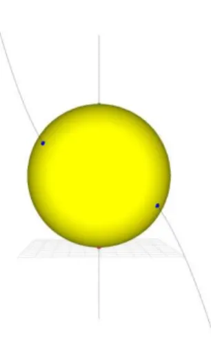
For any smooth parametric surface, we exhibit the implicit equation P = 0 of the singular curve P encoding all ridges of the surface (blue and red), and show how to recover the

SA153 qRT-PCR screening; Acetoin production screening; Acetoin monitoring in co-culture; Production of SA supernatant 3 Coexistence (SA2599, SA2597) Competition (SA2599,

Une faible production de l’AIA par les isolats a été enregistrée en absence de L- tryptophane dans le milieu de culture (2,878µg/ml), par ailleurs, la capacité

Nous allons examiner de plus près ces deux points. On notera au préalable qu’ils ont en commun de partir d’une conception empirique du sujet. En rattachant le sujet de la volonté à

Nous avons envisagé une décomposition plus fine de cette variable en distinguant : la variable de signal bce-rv révélatrice du résultat de la réunion du

En 1979 l’IC détaillait 871 catégories d’équipement contre 185 en 2014 dans la Base Permanente des Équipements (BPE).L’IC était aussi renseigné de façon variable : en 1979

Coefficients of fractional parentage are most conve- niently studied by sum-rule methods. The intermediate state expansion is usually given in terms of coupled