HAL Id: hal-02314025
https://hal.archives-ouvertes.fr/hal-02314025
Submitted on 11 Oct 2019
HAL is a multi-disciplinary open access
archive for the deposit and dissemination of
sci-entific research documents, whether they are
pub-lished or not. The documents may come from
teaching and research institutions in France or
abroad, or from public or private research centers.
L’archive ouverte pluridisciplinaire HAL, est
destinée au dépôt et à la diffusion de documents
scientifiques de niveau recherche, publiés ou non,
émanant des établissements d’enseignement et de
recherche français ou étrangers, des laboratoires
publics ou privés.
Combining Kriging and Controlled Stratification to
Identify Extreme Levels of Electromagnetic Interference
T. Houret, Philippe Besnier, S Vauchamp, P. Pouliguen
To cite this version:
T. Houret, Philippe Besnier, S Vauchamp, P. Pouliguen. Combining Kriging and Controlled
Stratifi-cation to Identify Extreme Levels of Electromagnetic Interference. 2019 International Symposium on
Electromagnetic Compatibility, EMC EUROPE, Sep 2019, Barcelone, Spain. �hal-02314025�
Combining Kriging and Controlled Stratification to Identify Extreme
Levels of Electromagnetic Interference
T. Houret
1,2, P. Besnier
1, S. Vauchamp
2, P. Pouliguen
31INSA Rennes, CNRS, IETR UMR 6164, F-35000 Rennes, France 2CEA DAM, F-46500, Gramat, France
3
DGA DGA/DS/MRIS, F-75009, Paris, France
Abstract— EMC risk analysis requires various configurations
of coupling paths described by important sets of unknown or uncertain parameters. More specifically, values at risk corresponding to extreme values of relevant fields, currents or voltages are often the most important information with regard to a possible EMC risk. Therefore, we aim at estimating extreme quantiles of the relevant field, current or voltage. Controlled stratification accelerates the standard Empirical estimation convergence to sample output extreme values, thus reducing the required number of calls to cost-expensive full-wave simulations. However, controlled stratification requires a simple (i.e. fast calculation time) model with sufficient correlation to the initial model. The main idea in this communication is to use a surrogate model as a simple model. Kriging was previously identified as a surrogate model with relevant properties. In this paper, we investigate the performance of combined kriging and control stratification. We show that this combination outperforms the stand-alone kriging surrogate model for estimating extreme quantiles. On the contrary, the latter performs better to identify less extreme quantiles.
Keywords— Uncertainty propagation; Extreme Quantiles Estimation; Monte Carlo; Kriging; Controlled Stratification
I. INTRODUCTION
EMC risk analysis, in the context of intentional electromagnetic interference (IEMI), often requires solving Maxwell equations with 3D numerical solvers based for instance on the method of moments or the finite difference time domain. Such models are deterministic and may be considered to provide “exact” solutions, but are very time consuming. At system-level EMC analysis, many input data are not well known due to epistemic uncertainties. These uncertainties propagate through the model. As a result, the calculated output exhibits non tractable fluctuations and may be described as a random variable. A proper IEMI risk assessment requires estimation of some extreme quantiles of the output for some input distributions. Finally, the knowledge of extreme quantile levels of aggression and of susceptibility levels informs about the probability of failure.
The Empirical Estimation (EE) is the standard approach to retrieve the output distribution. This approach is simple and very robust but converges very slowly, especially if extreme values are targeted. Surrogate models (SMs) are functions that approximate the true model (physical phenomena) and may be calculated from a much more reduced set of realizations. Once trained, they have a negligible computational cost compared to the model. Accurate SMs offer very good alternatives to a standard EE approach. Once the SM is trained, the output
distribution can be estimated by propagating the uncertainty through the SM as a substitute of the model.
SMs can also be used in addition to reliability technics such as Subset Simulation [1], Importance Sampling [2], that besides, can work without a SM. In other words, stand-alone SMs are not specifically dedicated to target the output distribution tail. On the contrary, Controlled Stratification (CS) [3] is dedicated to target extreme events, and requires a simple correlated model. This is possibly a SM as we propose in this paper. Note that CS has been successfully applied to a spring-mass-damper problem with splines as SM [4] and to an EMC crosstalk problem with a simple model which was not a SM [5].
Many probabilistic SMs exist, with many variants. In a recent paper [6], we showed that kriging [7] was the best candidate for CS as well as Polynomial Chaos Expansion (PCE)-kriging [8]. But computation time of the PCE part of the latter delays considerably the SM training. The kriging can also be improved by adaptively sampling the input space [9]. The time spent to train the adaptive kriging becomes prohibitive for large input samples. Accordingly, we chose the kriging as SM.
In this study, our purpose is to produce a cost-effective solution to determine extreme quantile estimation with a reasonable uncertainty or variance. The quantile estimation performance of the proposed combined Kriging and Controlled Stratification (K-CS) approach is compared to EE and kriging. To our knowledge, the K-CS has not yet been introduced to produce an IEMI risk assessment. A first specific case study with high non-linearity is used for the theoretical assessment of this new approach. Then, we deal with a second case study, which is analyzed as would be done in practice. Our purpose is to, not only demonstrate the performances of the K-CS, but also to provide a framework, easily reusable for practical applications.
This paper is organized as follow. First, a brief overview of kriging and CS are provided in section II. Then, we provide an evaluation of K-CS performance in section III based on the first specific case study mentioned above. The last section deals with the practical implementation of the method on a second case study. Finally, a conclusion and perspectives are given.
II. THEORETICAL BACKGROUND
A. Goal and procedure overview
Most physical phenomena studied in engineering can be modeled. A model is a function M that enables to predict an output Y given the input X:
Y=M(X) (1)
The model M is considered as an exact description of the physical phenomenon. It is typically time expensive. For instance, most EMC problems require full-wave simulations with many input parameters. Due to epistemic uncertainties, the input X is uncertain. The input may be therefore considered as a multivariate random variable. The uncertainty propagates through the model and therefore the output Y is also defined as a random variable (univariate in this paper but could be multivariate).
The goal is to compute a quantile qε of the cumulative
distribution function (cdf) of the output Y written as FY(y). By
definition, qε is related to the cdf: ( ) ) (y PY q FY (2)
Estimating the quantile can be summarized with the following three main steps:
1) Sample n realizations of the multivariate input. From those realizations, use the model to compute these n realizations of the output using the model. This first step is called the Design of Experiment (DOE). The sampling quality is important. We chose the well-known Latin Hypercube Sampling (LHS) [10].
2) Estimate the cdf of the output: Fˆ yY( ). We used in this paper three methods:
Empirical Estimation.
Surrogate modeling (kriging).
Controlled Stratification based on kriging.
3) Estimate the targeted quantile, which is straightforward once the second step is done:
) ( ˆ ˆ 1 FY q (3)
In the following, we undertake a fair comparison between the K-CS approach and the two other approaches. To do so, the total number of the true model calls (n) has to be exactly the same for all of them.
The computations were done on an AMD® Ryzen 7 1700x 8-cores processor, 16 threads machine, working at 3.4-3.8GHz. The implementation was coded in Matlab 2018 with the “UQLab” Framework [11], developed by Stefano Marelli and Bruno Sudret at ETH Zurich. Additionally, we used the following Matlab toolboxes: “Optimization”, “Global
Optimization”, “Statistics and Machine Learning” and “Parallel Computing”.
B. Empirical Estimation(EE)
From the DOE sample (of size n), the output sample is ordered and the empirical cdf is computed. Finally, a linear interpolation is made between sampled points. We used the Matlab function “quantile”, implementing that technique.
EE is a simple and robust technique, but needs a very large DOE to estimate extreme quantiles with accuracy.
C. Surrogate Modeling
The goal of a SM is to approximate the model. The function M’ of the SM is:
) ( ˆM' X
Y
Y (4)
Once the SM is built up from the DOE of size n, the SM may predict an unlimited number of output realizations at little cost while being accurate. Therefore, we use one million of predicted outputs to estimate the empirical quantile.
The Kriging was implemented using “UQLab”[12] with the following parameters:
Trend: constant (ordinary kriging).
Correlation family: Matern 5_2.
Estimation method: Maximum likelihood.
Optimization method: Hybrid Genetic Algorithm and gradient with a maximum of 200 iterations.
D. Controlled Stratification(CS)
CS is a technique dedicated to find extreme quantiles. CS samples the input space in order to generate more extreme output events in much less trials than direct sampling (i.e. with EE).
CS requires beforehand a correlated simple model. In our case, this simple model is a kriging SM. From the total simulation budget of n, nSM is reserved for building the SM and
the remaining nCS are used for the CS. We chose arbitrary: 2 n nSM (5)
The SM, once built, is used to predict a large number of output realizations. The predicted output sample is stratified, or sliced, hence the name “stratification”. The strata limits are SM quantiles estimation, thus the adjective “controlled”:
1 .... 0 , ] qˆ , … , qˆ [ 0 0 s s n n (6)
The number of strata (ns) is arbitrary as well as the stratum
limits, except 𝑞̂𝛼1 (or for upper tail 𝑞̂𝛼𝑛𝑠−1 ) which has to be the
ε targeted quantile. We used 4 strata and two different limits sets according to lower tail or upper tail quantile identification:
{ 𝑙𝑜𝑤𝑒𝑟 𝑡𝑎𝑖𝑙: [𝑞̂0, 𝑞̂𝜀, 𝑞̂2𝜀, 𝑞̂0.5, 𝑞̂1], 𝜀 < 0.25
𝑢𝑝𝑝𝑒𝑟 𝑡𝑎𝑖𝑙: [𝑞̂0, 𝑞̂0.5, 𝑞̂1−2(1−𝜀), 𝑞̂𝜀, 𝑞̂1], 𝜀 > 0.75 (7) CS has a budget of ncs points. Each stratum has a dedicated
s s CS s CS j s s CS j n j tail upper j tail lower n n n n N n j n n N : 1 : , ) , mod( ] , 2 [ , (8)
A more advanced allocation strategy based on an adaptive allocation of the number of points is also possible. However, adaptive allocation relies on the estimation of the optimal allocation, which does not always warrant performance improvement, in contrast with the uniform strategy [13].
The SM identifies Nj output realizations (j)
Yˆ belonging to the jth stratum. The model is called for each identified input in order to computeY(j). If the correlation (as defined in [3]) is high, most of the Y(j)remains in the jth stratum of the exact model. In fact, CS performance relies more on the high correlation associated to input sensitivity between the SM and the model than on the accuracy of SM prediction. In such conditions, an input producing an extreme event with the SM is likely to produce also an extreme event of the true model. Finally, the output estimated cdf is computed:
ns j N i y Y j j j Y j j i N y F 1 1 1 1 () 1 ) ( ˆ (9)III. PERFORMANCES COMPARISON
A. Presentation of the model
The true model is the reflection coefficient of a RLC serial circuit given by:
𝑌 = |𝑅 + 𝑗2𝜋𝑓 (𝐿 − 1
𝐶(2𝜋𝑓)2) − 50 𝑅 + 𝑗2𝜋𝑓 (𝐿 −𝐶(2𝜋𝑓)1 2) + 50
| (10)
The 4 random inputs are: the frequency (f ), the resistance (R), the capacitor (C) and the inductance (L).
The frequency is uniformly distributed from 100 to 900
MHz. The resistance, capacitor and inductance are uniformly
distributed between 90% and 110% of their nominal values. The nominal values (R=50 Ω, C=1.5 pF and L=67.5 nH) are chosen to reach a perfect resonance at 500 MHz. This test case is not a realistic one. However, it is used as a challenging test with regard to the high non-linearity of this resonating circuit.
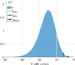
The model output distribution is plotted in Fig. 1 from a reference sample of 106 output realizations. So many realizations were computable because the model is analytical. The reference sample empirical distribution with 95% confidence bounds can be computed with Matlab function
“ecdf”. From the lower and upper bound, the precision of a
given quantile can be deduced. For q10% and q1%, the precision
is ±0.55% and ±1.1%, respectively. As the probability decreases, there are fewer realizations amongst the reference sample that are below the quantile. That is why the precision is lower for more extreme quantiles. These precisions are still far better than expected by all methods we deal with in this paper,
which use much less realizations. Hence, the quantiles from the reference sample are considered as true.
Fig. 1. Reflection coefficient model: Histogram of 106 responses of the true
model with the true quantiles that will be estimated.
B. Methodology, implementation details
1) Algoritm details for performance assessment
In this section III, our purpose is to investigate the spread of the estimated quantile. For EE, kriging, and K-CS approaches, we perform Monte Carlo simulations of the 3 steps introduced in section II.
For each Monte Carlo simulation (32 in total), we perform the 4 following phases of calculation:
1. Get a DOE of size n.
2. Estimate the targeted quantile with the three methods
(EE, kriging, K-CS).
3. Compute the relative error between the estimated and
the true quantile:
𝐸𝑟𝑟 =𝑞̂𝜀− 𝑞𝜀
𝑞𝜀 ⋅ 100 (11)
4. Compute the statistics of Err for the three methods.
2) Performance assessment
The chosen statistics to compare the errors (Err) are:
The mean error :
Err
1 ˆ (12)
The maximal absolute error:
𝜃2= 𝜇̂|𝐸𝑟𝑟| + 1.96 ⋅ 𝜎̂|𝐸𝑟𝑟 | (13)
TABLE I. TIME SPENT TO ESTIMATE ONCE A QUANTILE WITH KRIGING
DOE size 100 200 400 800 1600 3200 6400
Time (min) 0.42 0.47 0.65 1.28 3.54 12.81 106.3
Each Monte Carlo simulation takes time especially for large DOE sizes. For example, we report in Table I, the time spent for one Monte Carlo simulation with kriging for different DOE sizes. As a consequence, we had to limit to 32 Monte Carlo simulations. Therefore, we have only 32 error realizations. The
inference of θ1 and θ2is done with bootstrapping [14] and a kernel fit [15] thanks to the Matlab functions “bootstrap” and
“ksdensity”.
The bootstrapping technique is a resampling method with replacement to retrieve a distribution of a statistic. We resampled 1000 subsamples from the original 32 errors samples, computed the statistics on each of them to achieve 1000 realizations of θ1 and θ2. The histogram of those realizations is fitted to a kernel density. Finally, a 95% confidence interval, as well as the most likely realization (highest point of the θ1and θ2 kernelpdf), can be deduced from
the kernel distribution.
C. Results of quantile estimation
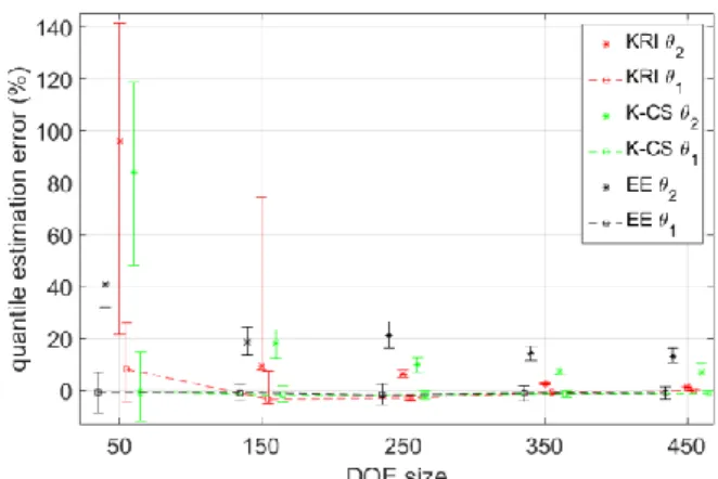
In Fig. 2 and Fig. 3, we plot the estimator of the mean of the errors θ1 andthe estimator of the maximal error θ2 for various DOE sizes when the targeted quantile is q10% and q1%.
The maximal likelihood of the statistic estimators are plotted with uncertainty bars corresponding to the 95% confidence interval.
In both plots, for every method, the maximal likelihood of θ1 and θ2and their uncertainty decreases when increasing the DOE size.
1) Ordinary quantile (q10%)
In Fig. 2, one can distinguish two regions of n:
1. n=[50,150]: No method performs very well (risk of high θ2 values). Note that θ1 for kriging is positively biased for n=50.
2. n=[250,350,450]: θ2for kriging is much lower than θ2 for CS. Therefore, kriging performs better than K-CS.
2) Extreme quantile (q1%)
In Fig. 3, one can distinguish two regions of n:
1. n=[1000]: None of the three methods perform well. Note that θ1 forkriging is very strongly positively biased.
2. n=[2000,3000,4000]: kriging θ2 is similar to EE θ2,
whereas θ2 for CS is much lower. Moreover, θ1 obtained from kriging is still strongly biased. Therefore, K-CS outperforms both EE and kriging. The model is strongly non-linear because of the resonance phenomenon. The DOE size needed to reach reasonable accuracy is very large. As a consequence, the time spent to build a kriging is not negligible as shown in Table I. Because the K-CS needs only half of the DOE size needed for kriging, the time spent for the K-CS is much reduced compared to the stand alone kriging.
We may therefore conclude that K-CS is well fitted to estimate extreme quantiles.
Fig. 2. Reflection coefficient q10% estimation. Mean relative error (θ1) and
maximum absolute relative error (θ2) with: Empirical Estimation (EE), kriging (KRI) and kriging+controlled stratification (K-CS).
Fig. 3. Reflection coefficient q1% estimation. Mean relative error (θ1) and
maximum absolute relative error (θ2) with: Empirical Estimation (EE), kriging (KRI) and kriging+controlled stratification (K-CS).
IV. EMC APPLICATION CASE
A. Presentation of the model
The model is the electrical far-field magnitude radiated by a PCB trace, loaded at each end, above an infinite ground plane. See the schematic in Fig. 4.
Fig. 5. PCB radiation model: Histogram of the 106 responses of the PCB
radiation true model and the true quantiles that will be estimated.
The 11 random variable inputs are: the frequency (f), geometrical characteristics (the substrate thickness (h), the trace width/length W/l), electrical characteristics (substrate permittivity εr, voltage source Vs, impedance source Zs,
impedance load Zl), and the position where the field is
measured (spherical coordinates r, θ, and φ). Each input follows a Gaussian distribution centered at their nominal value with a relative standard deviation of 10%. The nominal values are chosen so the trace appears as a quarter wavelength transmission line: f=404 MHz, h=0.775 mm, W=0.51 cm,
l=10.16 cm, εr=4.6, Vs=1 V, Zs=50 Ω, Zl=1 Ω, r=3 m, φ= θ=
2π.
The model output is the radiated field magnitude computed from (23) in [16]. The histogram of the output reference sample (106 realizations) is plotted in Fig. 5 with three true quantiles. The estimated precision of q90%, q99%, q99.9% is
respectively ±0.0093%, ±0.019% and ±0.044%. This precision is computed like in the 3rd § in section III.A.
B. Methodology, implementation details
The methodology is similar to section III excepting error estimation. This case study being an application case, Monte Carlo simulations are not performed. A single error is therefore calculated for a given DOE size. Indeed, in practice, a single budget of n simulations is allowed. We then study the quantile estimation convergence as a function of the DOE size.
1) Algoritm details for performance assessment
The algorithm implemented for the application case follows the first three steps introduced in section III.
2) Performance assessment
The error as a function of the DOE size exhibits large statistical fluctuations. It is not possible, strictly speaking, to group some realizations in order to infer a statistic (e.g. the mean) because they are not sampled from the same distribution. However we assume that this is the case for close DOE sizes. We used an averaging sliding window of size of 30 to smooth the noise of the errors with Matlab function
“movmean”.
In practice, the true quantile will not be available. The proposed framework would need a small adjustment and an optimization algorithm. Instead of errors, only the estimated quantile will be available. An optimization algorithm would have to find the DOE size when the quantile estimator presents small variations. The convergence is then reached. The best suited algorithm, the variation estimator, and an acceptable criterion have yet to be defined.
C. Results: comparison quantile estimation
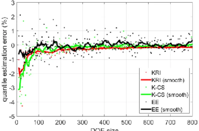
Fig. 6, Fig. 7, Fig. 8 are plots of the errors when estimating
q90%, q99%, and q99.9%, respectively. The dot points represent
error realizations while solid lines represent the smoothed errors described in section II.B.2.
In each plot, for every method, the smoothed errors converge to 0, and the realizations are less spread as the DOE size increases.
1) Ordinary quantile (q90%)
In Fig. 6, there are two domains for n:
1. n≤100: None of the three methods performs well. 2. n>100: EE is still clearly the worst due to its very large
spread from 0. K-CS mean error is closer to zero than kriging mean error, but has some rare but high errors. Kriging presents a small but clear negative bias. The two methods perform equally.
2) Extreme quantile (q99%)
In Fig. 7, there are two domains for n:
1. n≤200: None of the three methods performs well. 2. n>200: EE is still the worst method. Kriging is still
biased but with low spread. K-CS is unbiased with low spread but there are very few high errors. K-CS starts to outperform the stand-alone kriging.
3) Very extreme quantile (q99.9%)
In Fig. 8, the domains limits are shifted upward. The first is now: n≤350 and the second: n>350. K-CS clearly outperforms both EE and kriging.
Fig. 6. PCB radiation q90% estimation. Relative error (%) with: Empirical
Fig. 7. PCB radiation q99% estimation: relative error (%) with: Empirical
Estimation (EE), kriging (KRI) and kriging + controlled stratification (K-CS).
Fig. 8. PCB radiation q99.9% estimation: relative error (%) with: Empirical
Estimation (EE), kriging (KRI) and kriging + controlled stratification (K-CS).
V. CONCLUSION
In this paper we introduced the controlled stratification based on kriging (K-CS) and compared it with Empirical Estimation (EE) and kriging (KRI) to estimate an extreme quantile of an output distribution.
Through a Monte Carlo analysis of the three methods for a reference model (RLC circuit reflection coefficient) with high non-linearity we showed that the new K-CS method proposed in this paper outperforms the two other methods, especially the stand-alone kriging approach, for extreme quantiles estimation.
Then, an EMC case study application (PCB radiation) has been used to investigate the convergence of K-CS as a function of the DOE size. The performance of K-CS approach is confirmed for extreme quantiles. On the contrary, a stand-alone kriging approach suffices for not too extreme quantiles.
The K-CS becomes more relevant than kriging when estimating q1% of the reflection coefficient. For the PCB
radiation model, the K-CS becomes a better solution when estimating q99.9%.Therefore, K-CS outperforms kriging for less
extreme quantiles as non-linearity of the model (in the extreme values region) increases.
In the context of IEMI risk analysis and the determination of low probability risk of failure the K-CS is therefore relevant to reach an acceptable approximation with a limited DOE size.
For very high dimension models, the time building the Kriging may become important. In that case, model order reduction techniques like Partial Least Square [17] could be used.
ACKNOWLEDGMENT
The authors would like to thank the support from the Délégation Générale de l’Armement.
REFERENCES
[1] X. Huang, J. Chen, and H. Zhu, “Assessing small failure probabilities by AK–SS: An active learning method combining Kriging and Subset Simulation,” Struct. Saf., vol. 59, pp. 86–95, Mar. 2016.
[2] B. Echard, N. Gayton, M. Lemaire, and N. Relun, “A combined Importance Sampling and Kriging reliability method for small failure probabilities with time-demanding numerical models,” Reliab. Eng.
Syst. Saf., vol. 111, pp. 232–240, Mar. 2013.
[3] C. Cannamela, J. Garnier, and B. Iooss, “Controlled stratification for quantile estimation,” Ann. Appl. Stat., vol. 2, no. 4, pp. 1554–1580, Dec. 2008.
[4] G. C. Enss, M. Kohler, A. Krzyzak, and R. Platz, “Nonparametric Quantile Estimation Based on Surrogate Models,” IEEE Trans. Inf.
Theory, vol. 62, no. 10, pp. 5727–5739, Oct. 2016.
[5] M. Larbi, P. Besnier, and B. Pecqueux, “The Adaptive Controlled Stratification Method Applied to the Determination of Extreme Interference Levels in EMC Modeling With Uncertain Input Variables,” IEEE Trans. Electromagn. Compat., vol. 58, no. 2, pp. 543–552, Apr. 2016.
[6] T. Houret, P. Besnier, S. Vauchamp, and P. Pouliguen, “Comparison of Surrogate Models for Extreme Quantile Estimation in the Context of EMC Risk Analysis,” presented at the APEMC, Sapporo, 2019. [7] C. E. Rasmussen and C. K. I. Williams, Gaussian processes for
machine learning, 3. print. Cambridge, Mass.: MIT Press, 2008.
[8] R. Schobi, B. Sudret, and J. Wiart, “POLYNOMIAL-CHAOS-BASED KRIGING,” Int. J. Uncertain. Quantif., vol. 5, no. 2, pp. 171–193, 2015.
[9] J. Zhang and A. A. Taflanidis, “Adaptive Kriging Stochastic Sampling and Density Approximation and Its Application to Rare-Event Estimation,” ASCE-ASME J. Risk Uncertain. Eng. Syst. Part Civ.
Eng., vol. 4, no. 3, p. 04018021, Sep. 2018.
[10] M. Stein, “Large Sample Properties of Simulations Using Latin Hypercube Sampling,” Technometrics, vol. 29, no. 2, p. 143, May 1987.
[11] S. Marelli and B. Sudret, “UQLab: A Framework for Uncertainty Quantification in Matlab,” in Vulnerability, Uncertainty, and Risk, Liverpool, UK, 2014, pp. 2554–2563.
[12] R. Schöbi, S. Marelli, and B. Sudret, “UQLab user manual – Kriging (Gaussian process modelling).” 2017.
[13] M. Larbi, “Méthodes statistiques pour le calcul d’interférences électromagnétiques extrêmes au sein de systèmes complexes,” thesis, Rennes, INSA, 2016.
[14] E. S. Banjanovic and J. W. Osborne, “Confidence Intervals for Effect Sizes: Applying Bootstrap Resampling,” Practical Assessment,
Research & Evaluation.
[15] B. W. Silverman, Density estimation for statistics and data analysis, 1., CRC Press repr. Boca Raton, Fla.: Chapman & Hall/CRC, 1986. [16] M. Leone, “Closed-Form Expressions for the Electromagnetic
Radiation of Microstrip Signal Traces,” IEEE Trans. Electromagn.
Compat., vol. 49, no. 2, pp. 322–328, May 2007.
[17] M. A. Bouhlel, N. Bartoli, A. Otsmane, and J. Morlier, “Improving kriging surrogates of high-dimensional design models by Partial Least Squares dimension reduction,” Struct. Multidiscip. Optim., vol. 53, no. 5, pp. 935–952, May 2016.